Scaling-up Empirical Risk Minimization: Optimization of Incomplete U-statistics
In a wide range of statistical learning problems such as ranking, clustering or metric learning among others, the risk is accurately estimated by $U$-statistics of degree $d\geq 1$, i.e. functionals of the training data with low variance that take th…
Authors: Stephan Clemenc{c}on, Aurelien Bellet, Igor Colin
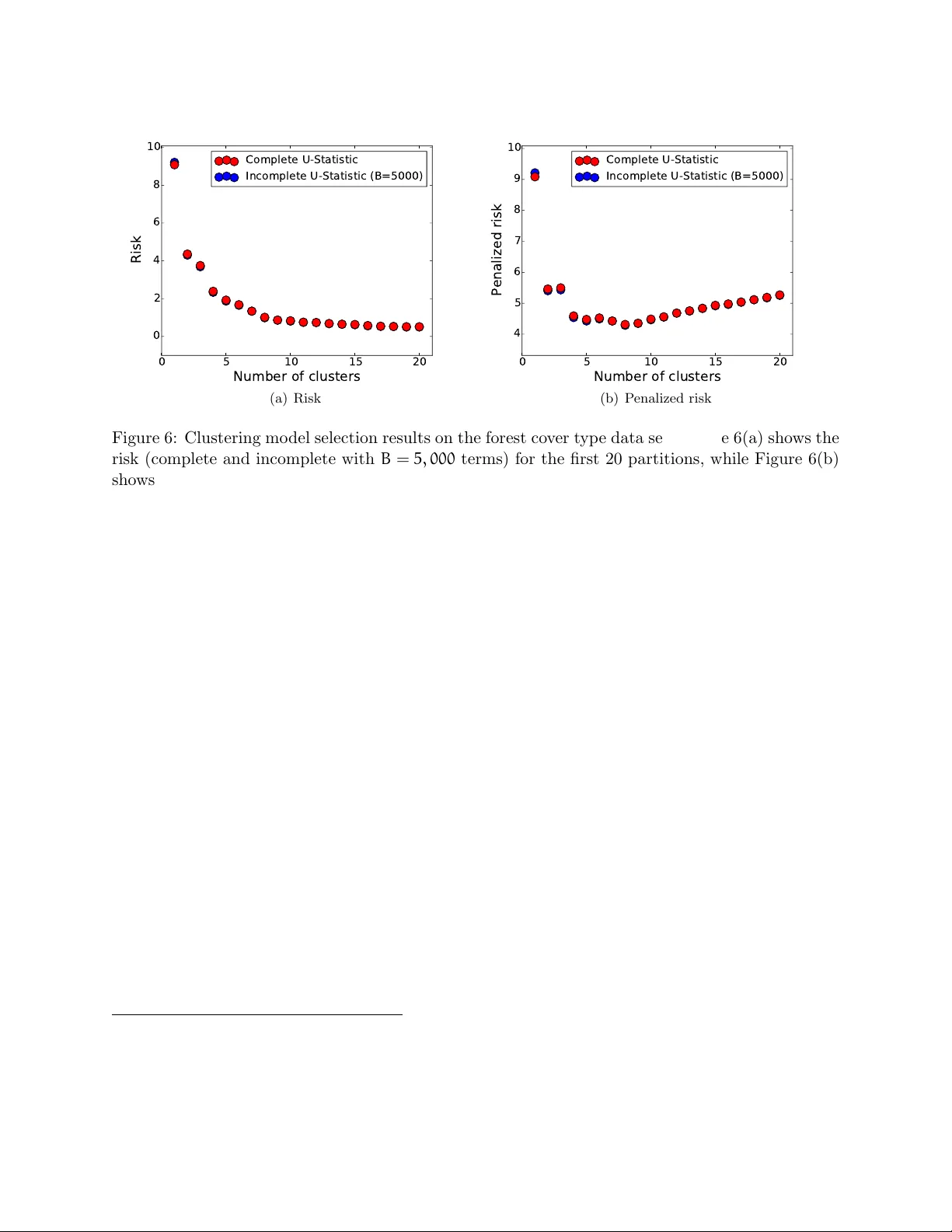
Scaling-up Empirical Risk Minimization: Optimization of Incomplete U -statistics St ´ ephan Cl ´ emen¸ con ∗ , Aur ´ elien Bellet † , Igor Colin ∗ April 20, 2016 Abstract In a wide range of statistical learning problems suc h as ranking, clustering or metric learning among others, the risk is accurately estimated by U -statistics of degree d ≥ 1 , i.e. function- als of the training data with lo w v ariance that take the form of av erages o ver k -tuples. F rom a computational p ersp ectiv e, the calculation of suc h statistics is highly expensive even for a mo derate sample size n , as it requires a veraging O ( n d ) terms. This makes learning procedures relying on the optimization of suc h data functionals hardly feasible in practice. It is the ma jor goal of this paper to sho w that, strikingly , suc h empirical risks can b e replaced by drastically computationally simpler Mon te-Carlo estimates based on O ( n ) terms only , usually referred to as inc omplete U -statistics , without damaging the O P ( 1/ √ n ) learning rate of Empiric al Risk Mini- mization (ERM) pro cedures. F or this purpose, w e establish uniform deviation results describing the error made when approximating a U -process b y its incomplete v ersion under appropriate complexit y assumptions. Extensions to mo del selection, fast rate situations and v arious sam- pling techniques are also considered, as well as an application to sto c hastic gradient descent for ERM. Finally , numerical examples are displa y ed in order to provide strong empirical evidence that the approac h w e promote largely surpasses more naiv e subsampling techniques. 1 In tro duction In classification/regression, empirical risk es timates are sample mean statistics and the theory of Empiric al Risk Minimization (ERM) has b een originally developed in this con text, see Devroy e et al. (1996). The ERM theory essentially relies on the study of maximal deviations b et ween these empirical av erages and their exp ectations, under adequate complexit y assumptions on the set of prediction rule candidates. The relev an t to ols are mainly concen tration inequalities for empirical pro cesses, see Ledoux and T alagrand (1991) for instance. In a wide v ariety of problems that receiv ed a goo d deal of atten tion in the mac hine learning literature and ranging from clustering to image recognition through ranking or learning on graphs, natural estimates of the risk are not basic sample means but take the form of av erages of d -tuples, usually referred to as U -statistics in Probabilit y and Statistics, see Lee (1990). In Cl ´ emen¸ con et al. (2005) for instance, ranking is view ed as pairwise classification and the empirical ranking error of any giv en prediction rule is a U -statistic of order 2 , just lik e the within cluster p oint ∗ L TCI, CNRS, T´ el ´ ecom P arisT ec h, Univ ersit´ e Paris-Sacla y , 75013, Paris, F rance. { stephan.clemencon,igor.colin } @telecom-paristech.fr † Magnet T eam, INRIA Lille – Nord Europe, 59650 Villeneuve d’Ascq, F rance. aurelien.bellet@inria.fr 1 sc atter in cluster analysis (see Cl´ emen¸ con, 2014) or empirical p erformance measures in metric learning, refer to Cao et al. (2012) for instance. Because empirical functionals are computed b y a v eraging o v er tuples of sampling observ ations, they exhibit a complex dep endence structure, whic h appears as the price to b e paid for low v ariance estimates. Line arization te chniques (see Ho effding, 1948) are the main ingredient in studying the b eha vior of empirical risk minimizers in this setting, allo wing to establish probabilistic upp er b ounds for the maximal deviation of collection of centered U -statistics under appropriate conditions b y reducing the analysis to that of standard empirical pro cesses. How ever, while the ERM theory based on minimization of U -statistics is no w consolidated (see Cl´ emen¸ con et al., 2008), putting this approach in practice generally leads to significant computational difficulties that are not sufficien tly well do cumen ted in the mac hine learning literature. In many concrete cases, the mere computation of the risk inv olves a summation o v er an extremely high num b er of tuples and runs out of time or memory on most mac hines. Whereas the av ailability of massiv e information in the Big Data era, whic h machine learning pro cedures could theoretically now rely on, has motiv ated the recent developmen t of p ar al lelize d / distribute d approac hes in order to scale-up certain statistical learning algorithms, see Bekkerman et al. (2011) or Bianc hi et al. (2013) and the references therein, the present pap er prop oses to use sampling te chniques as a remedy to the apparen t intractabilit y of learning from data sets of explosiv e size, in order to break the current computational barriers. More precisely , it is the ma jor goal of this article to study ho w a simplistic sampling tec hnique ( i.e. dra wing with replacemen t) applied to risk estimation, as originally prop osed b y Blom (1976) in the context of asymptotic point wise estimation, ma y efficiently remedy this issue without damaging to o m uc h the “reduced v ariance” prop ert y of the estimates, while preserving the learning rates (including certain ”fast-rate” situations). F or this purp ose, we inv estigate to which exten t a U -pro cess, that is a collection of U -statistics, can b e accurately approximated b y a Monte-Carlo version (which shall b e referred to as an inc omplete U -pr o c ess throughout the pap er) inv olving m uch less terms, provided it is indexed b y a class of k ernels of con trolled complexit y (in a sense that will be explained later). A maximal deviation inequalit y connecting the accuracy of the approximation to the num b er of terms in volv ed in the appro ximan t is th us established. This result is the k ey to the analysis of the statistical p erformance of minimizers of risk estimates when they are in the form of an incomplete U -statistic. In particular, this allo ws us to show the adv antage of using this sp ecific sampling technique, compared to more naiv e approaches with exactly the same computational cost, consisting for instance in first drawing a subsample and then computing a risk estimate of the form of a (complete) U -statistic based on it. W e also sho w ho w to incorp orate this sampling strategy in to iterativ e statistical learning techniques based on stochastic gradien t descent (SGD), see Bottou (1998). The v ariant of the SGD metho d w e prop ose inv olves the computation of an incomplete U -statistic to estimate the gradien t at eac h step. F or the estimator thus pro duced, rate b ounds describing its statistical p erformance are established under mild assumptions. Beyond theoretical results, w e present illustrative n umerical exp erimen ts on metric learning and clustering with synthetic and real-w orld data that supp ort the relev ance of our approac h. The rest of the article is organized as follo ws. In Section 2, we recall basic definitions and con- cepts p ertaining to the theory of U -statistics/processes and present important examples in mac hine learning where natural estimates of the p erformance/risk measure are U -statistics. W e then review the existing results for the empirical minimization of complete U -statistics. In Section 3, we recall the notion of incomplete U -statistic and we deriv e maximal deviation inequalities describing the error made when approximating a U -statistic by its incomplete counterpart uniformly ov er a class 2 of kernels that fulfills appropriate complexity assumptions. This result is next applied to derive (p ossibly fast) learning rates for minimizers of the incomplete v ersion of the empirical risk and to mo del selection. Extensions to incomplete U -statistics built b y means of other sampling schemes than sampling with replacement are also in vestigated. In Section 4, estimation b y means of incom- plete U -statistics is applied to sto c hastic gradien t descen t for iterativ e ERM. Section 5 presen ts some n umerical exp erimen ts. Finally , Section 6 collects some concluding remarks. T ec hnical details are deferred to the App endix. 2 Bac kground and Preliminaries As a first go, w e briefly recall some key notions of the theory of U -statistics (Section 2.1) and provide sev eral examples of statistical learning problems for which natural estimates of the p erformance/risk measure are in the form of U -statistics (Section 2.2). Finally , w e review and extend the existing rate b ound analysis for the empirical minimization of (complete) generalized U -statistics (Section 2.3). Here and throughout, N ∗ denotes the set of all strictly p ositiv e integers, R + the set of nonnegative real n umbers. 2.1 U -Statistics/Pro cesses: Definitions and Prop erties F or clarit y , w e recall the definition of generalized U -statistics. An excellen t account of prop erties and asymptotic theory of U -statistics can b e found in Lee (1990). Definition 1. (Generalized U -st a tistic) L et K ≥ 1 and ( d 1 , . . . , d K ) ∈ N ∗ K . L et X { 1, ..., n k } = ( X ( k ) 1 , . . . , X ( k ) n k ) , 1 ≤ k ≤ K , b e K indep endent samples of sizes n k ≥ d k and c omp ose d of i.i.d. r andom variables taking their values in some me asur able sp ac e X k with distribution F k ( dx ) r esp e c- tively. L et H : X d 1 1 × · · · × X d K K → R b e a me asur able function, squar e inte gr able with r esp e ct to the pr ob ability distribution µ = F ⊗ d 1 1 ⊗ · · · ⊗ F ⊗ d K K . Assume in addition (without loss of gener ality) that H ( x ( 1 ) , . . . , x ( K ) ) is symmetric within e ach blo ck of ar guments x ( k ) (value d in X d k k ), 1 ≤ k ≤ K . The gener alize d (or K -sample) U -statistic of de gr e es ( d 1 , . . . , d K ) with kernel H , is then define d as U n ( H ) = 1 Q K k = 1 n k d k X I 1 . . . X I K H ( X ( 1 ) I 1 , X ( 2 ) I 2 , . . . , X ( K ) I K ) , (1) wher e the symb ol P I k r efers to summation over al l n k d k subsets X ( k ) I k = ( X ( k ) i 1 , . . . , X ( k ) i d k ) r elate d to a set I k of d k indexes 1 ≤ i 1 < . . . < i d k ≤ n k and n = ( n 1 , . . . , n K ) . The ab o ve definition generalizes standard sample mean statistics, whic h corresp ond to the case K = 1 = d 1 . More generally when K = 1 , U n ( H ) is an av erage ov er all d 1 -tuples of observ ations, while K ≥ 2 corresp onds to the m ulti-sample situation with a d k -tuple for eac h sample k ∈ { 1, . . . , K } . A U -pro cess is defined as a collection of U -statistics indexed by a set H of kernels. This concept generalizes the notion of empirical pro cess. Man y statistics used for p oin twise estimation or hypothesis testing are actually generalized U -statistics ( e.g. the sample v ariance, the Gini mean difference, the Wilcoxon Mann-Whitney statistic, Kendall tau). Their p opularit y mainly arises from their “reduced v ariance” prop ert y: the 3 statistic U n ( H ) has minimum v ariance among all un biased estimators of the parameter µ ( H ) = E h H ( X ( 1 ) 1 , . . . , X ( 1 ) d 1 , . . . , X ( K ) 1 , . . . , X ( K ) d K ) i (2) = Z x ( 1 ) ∈X d 1 1 · · · Z x ( K ) ∈X d K K H ( x ( 1 ) , . . . , x ( K ) ) dF ⊗ d 1 1 ( x ( 1 ) ) · · · dF ⊗ d K K ( x ( K ) ) = E [ U n ( H ) ] . Classically , the limit prop erties of these statistics (law of large n umbers, cen tral limit theorem, etc. ) are inv estigated in an asymptotic framework stipulating that, as the size of the full p ooled sample n def = n 1 + . . . + n K (3) tends to infinity , w e hav e: n k /n → λ k > 0 for k = 1, . . . , K. (4) Asymptotic results and deviation/momen t inequalities for K -sample U -statistics can b e classically established by means of sp ecific representations of this class of functionals, see (15) and (27) in- tro duced in later sections. Significant progress in the analysis of U -statistics and U -pro cesses has then recently b een achiev ed by means of decoupling theory , see de la Pe˜ na and Gin´ e (1999). F or completeness, w e point out that the asymptotic b eha vior of (multisample) U -statistics has b een in v estigated under weak er integrabilit y assumptions than that stipulated in Definition 1, see Lee (1990). 2.2 Motiv ating Examples In this section, we review imp ortan t supervised and unsup ervised statistical learning problems where the empirical performance/risk measure is of the form of a generalized U -statistics. They shall serv e as running examples throughout the pap er. 2.2.1 Clustering Clustering refers to the unsup ervised learning task that consists in partitioning a set of data p oin ts X 1 , . . . , X n in a feature space X in to a finite collection of subgroups dep ending on their similarity (in a sense that must be sp ecified): roughly , data p oin ts in the same subgroup should b e more similar to eac h other than to those lying in other subgroups. One may refer to Chapter 14 in F riedman et al. (2009) for an account of state-of-the-art clustering tec hniques. F ormally , let M ≥ 2 b e the n um b er of desired clusters and consider a symmetric function D : X × X → R + suc h that D ( x, x ) = 0 for an y x ∈ X . D measures the dissimilarit y b et w een pairs of observ ations ( x, x 0 ) ∈ X 2 : the larger D ( x, x 0 ) , the less similar x and x 0 . F or instance, if X ⊂ R d , D could tak e the form D ( x, x 0 ) = Ψ ( k x − x 0 k q ) , where q ≥ 1 , || a || q = ( P d i = 1 | a i | q ) 1/q for all a ∈ R d and Ψ : R + → R + is any b orelian nondecreasing function such that Ψ ( 0 ) = 0 . In this con text, the goal of clustering metho ds is to find a partition P of the feature space X in a class Π of partition candidates that minimizes the following empiric al clustering risk : c W n ( P ) = 2 n ( n − 1 ) X 1 ≤ i 0 . F or any minimizer b H B of the statistic al estimate of the risk (19) , the fol lowing assertions hold true (i) We have with pr ob ability at le ast 1 − δ : ∀ n ∈ N ∗ K , ∀ B ≥ 1 , µ ( b H B ) − inf H ∈H µ ( H ) ≤ 2 M H × 2 r 2V log ( 1 + N ) N + r log ( 2/δ ) N + r 2 V log ( 1 + # Λ ) + log ( 4/δ ) B . (ii) We have: ∀ n ∈ N ∗ K , ∀ B ≥ 1 , E sup H ∈H e U B ( H ) − µ ( H ) ≤ M H 2 r 2V log ( 1 + N ) N + r 2 ( log 2 + V log ( 1 + # Λ )) B . The first assertion of Theorem 1 pro vides a con trol of the deviations b et ween the U -statistic (1) and its incomplete counterpart (19) uniformly ov er the class H . As the n um b er of terms B increases, this deviation decreases at a rate of O ( 1/ √ B ) . The second assertion of Theorem 1 gives a maximal deviation result with resp ect to µ ( H ) . Observe in particular that, with the asymptotic settings previously specified, N = O ( n ) and log ( # Λ ) = O ( log n ) as n → + ∞ . The b ounds stated ab o ve thus sho w that, for a num b er B = B n of terms tending to infinity at a rate O ( n ) as n → + ∞ , the maximal deviation sup H ∈H | e U B ( H ) − µ ( H ) | is asymptotically of the order O P (( log ( n ) /n ) 1/2 ) , just lik e sup H ∈H | U n ( H ) − µ ( H ) | , see b ound (17) in Proposition 1. In short, when considering an incomplete U -statistic (19) with B = O ( n ) terms only , the learning rate for the corresp onding minimizer is of the same order as that of the minimizer of the complete risk (1), whose computation requires to av erage # Λ = O ( n d 1 + ... + d K ) terms. Minimizing suc h incomplete U -statistics th us yields a significant gain in terms of computational cost while fully preserving the learning rate. In con trast, as implied by Prop osition 1, the minimization of a complete U -statistic in v olving O ( n ) terms, obtained by drawing subsamples of sizes n 0 k = O ( n 1/ ( d 1 + ... + d K ) ) uniformly at random, leads to a rate of con v ergence of O ( p log ( n ) /n 1/ ( d 1 + ... + d K ) ) , whic h is muc h slow er except in the trivial case where K = 1 and d 1 = 1 . These striking results are summarized in T able 1. The imp ortan t practical consequence of the ab o ve is that when n is to o large for the complete risk (1) to b e used, one should instead use the incomplete risk (19) (setting the n umber of terms B as large as the computational budget allo ws). 11 Empirical risk criterion Nb of terms Rate b ound Complete U -statistic O ( n d 1 + ... + d K ) O P ( p log ( n ) /n ) Complete U -statistic based on subsamples O ( n ) O P q log ( n ) /n 1 d 1 + ... + d K Incomplete U -statistic (our result) O ( n ) O P ( p log ( n ) /n ) T able 1: Rate bound for the empirical minimizer of sev eral empirical risk criteria versus the n umber of terms inv olved in the computation of the criterion. F or a computational budget of O ( n ) terms, the rate b ound for the incomplete U -statistic criterion is of the same order as that of the complete U -statistic, whic h is a huge improv ement ov er a complete U -statistic based on a subsample. 3.2 Mo del Selection Based on Incomplete U -Statistics Automatic selection of the mo del complexit y is a crucial issue in mac hine learning: it includes the n umber of clusters in cluster analysis (see Cl´ emen¸ con, 2014) or the c hoice of the num b er of p ossible v alues taken b y a piecewise constan t scoring function in m ultipartite ranking for instance ( cf. Cl ´ emen¸ con and V a yatis, 2009). In the presen t situation, this b oils down to c ho osing the adequate level of complexity of the class of k ernels H , measured through its (supp osedly finite) VC dimension for simplicit y , in order to minimize the (theoretical) risk of the empirical minimizer. It is the purp ose of this subsection to show that the incomplete U -statistic (19) can b e used to define a p enalization method to select a prediction rule with nearly minimal risk, a voiding procedures based on data splitting/resampling and extending the celebrated structur al risk minimization principle, see V apnik (1999). Let H b e the collection of all symmetric k ernels on Q K k = 1 X d k k and set µ ∗ = inf H ∈H µ ( H ) . Let H 1 , H 2 , . . . b e a sequence of uniformly b ounded ma jor sub classes of H , of increasing complexit y ( V C dimension). F or any m ≥ 1 , let V m denote the V C dimension of the class H m and set M H m = sup ( H,x ) ∈H m ×X | H ( x ) | < + ∞ . W e supp ose that there exists M < + ∞ suc h that sup m ≥ 1 M H m ≤ M . Giv en 1 ≤ B ≤ # Λ and m ≥ 1 , the complexity p enalized empirical risk of a solution e U B,m of the ERM problem (23) with H = H m is e U B ( b H B,m ) + pen ( B, m ) , (24) where the quantit y p en ( B, m ) is a distribution fr e e penalty given by: p en ( B, m ) = 2 M H m r 2V m log ( 1 + N ) N + r 2 ( log 2 + V m log ( 1 + # Λ )) B + 2 M r ( B + n ) log m B 2 . (25) As shown in Assertion ( ii ) of Corollary 1, the quan tit y abov e is an upp er b ound for the exp ected maximal deviation E [ sup H ∈H m | e U B ( H ) − µ ( H ) | ] and is thus a natural p enalt y candidate to comp en- sate the ov erfitting within class H m . W e thus prop ose to select b m B = arg min m ≥ 1 e U B ( b H B,m ) + pen ( B, m ) . (26) 12 As revealed b y the theorem b elo w, c ho osing B = O ( n ) , the prediction rule b H b m B based on a p enalized criterion in v olving the summation of O ( n ) terms solely , ac hiev es a nearly optimal trade-off b et w een the bias and the distribution free upp er b ound (25) on the v ariance term. Theorem 2. (Oracle inequality) Supp ose that The or em 1’s assumptions ar e fulfil le d for al l m ≥ 1 and that sup m ≥ 1 M H m ≤ M < + ∞ . Then, we have: ∀ n ∈ N ∗ K , ∀ B ∈ { 1, . . . , # Λ } , µ ( b H B, b m ) − µ ∗ ≤ inf k ≥ 1 inf H ∈H m µ ( H ) − µ ∗ + p en ( B, m ) + M p 2π ( B + n ) B . W e p oin t out that the argument used to obtain the ab o v e result can b e straightforw ardly extended to other (possibly data-dep enden t) complexit y p enalties ( cf. Massart, 2006), see the pro of in App endix D. 3.3 F ast Rates for ERM of Incomplete U -Statistics In Cl ´ emen¸ con et al. (2008), it has b een pro ved that, under certain “lo w-noise” conditions, the minim um v ariance prop ert y of the U -statistics used to estimate the ranking risk (corresp onding to the situation K = 1 and d 1 = 2 ) leads to learning rates faster than O P ( 1/ √ n ) . These results rely on the Hajek pr oje ction , a linearization technique originally introduced in Ho effding (1948) for the case of one sample U -statistics and next extended to the analysis of a muc h larger class of functionals in H´ ajek (1968). It consists in writing U n ( H ) as the sum of the orthogonal pro jection b U n ( H ) = K X k = 1 n k X i = 1 E h U n ( H ) | X ( k ) i i − ( n − 1 ) µ ( H ) , (27) whic h is itself a sum of K indep enden t basic sample means based on i.i.d. r.v.’s (of the order O P ( 1/ √ n ) each, after recen tering), plus a p ossible negligible term. This representation was used for instance b y Grams and Serfling (1973) to refine the CL T in the m ultisample U -statistics framew ork. Although useful as a theoretical to ol, it should be noticed that the quan tity b U n ( H ) is not of practical in terest, since the conditional exp ectations inv olved in the summation are generally unkno wn. Although incomplete U -statistics do not share the minimum v ariance property (see Section 3.1), w e will sho w that the same fast rate bounds for the excess risk as those reac hed b y ERM of U - statistics (corresponding to the summation of O ( n 2 ) pairs of observ ations) can b e attained by empirical ranking risk minimizers, when estimating the ranking risk b y incomplete U -statistics in v olving the summation of o ( n 2 ) terms solely . F or clarit y (and comparison purp ose), we first recall the statistical learning framew ork consid- ered in Cl ´ emen¸ con et al. (2008). Let ( X, Y ) b e a pair of random v ariables defined on the same probabilit y space, where Y is a real-v alued lab el and X mo dels some input information taking its v alues in a measurable space X hop efully useful to predict Y . Denoting by ( X 0 , Y 0 ) an indep enden t cop y of the pair ( X, Y ) . The goal pursued here is to learn how to rank the input observ ations X and X 0 , b y means of an an tisymmetric r anking rule r : X 2 → { − 1, + 1 } ( i.e. r ( x, x 0 ) = − r ( x 0 x ) for any ( x, x 0 ) ∈ X 2 ), so as to minimize the r anking risk L ( r ) = P { ( Y − Y 0 ) · r ( X, X 0 ) < 0 } . (28) The minimizer of the ranking risk is the ranking rule r ∗ ( X, X 0 ) = 2 I { P { Y > Y 0 | ( X, X 0 ) } ≥ P { Y < Y 0 | ( X, X 0 ) } − 1 (see Prop osition 1 in Cl´ emen¸ con et al., 2008). The natural empirical coun terpart 13 of (28) based on a sample of independent copies ( X 1 , Y 1 ) , . . . , ( X n , Y n ) of the pair ( X, Y ) is the 1 -sample U -statistic U n ( H r ) of degree tw o with kernel H r (( x, y ) , ( x 0 , y 0 )) = I { ( y − y 0 ) · r ( x, x 0 ) < 0 } for all ( x, y ) and ( x 0 , y 0 )) in X × R given by: L n ( r ) = U n ( H r ) = 2 n ( n − 1 ) X i 0 and α ∈ [ 0, 1 ] such that: ∀ r ∈ R , Var ( h r ( X, Y ) ) ≤ cΛ ( r ) α , wher e we set h r ( x, y ) = E [ q r (( x, y ) , ( X 0 , Y 0 )] . Recall incidentally that v ery general sufficien t conditions guaran teeing that this assumption holds true hav e b een exhibited, see Section 5 in Cl´ emen¸ con et al. (2008) (notice that the condition is void for α = 0 ). Since our goal is to explain the main ideas rather than achieving a high level of generalit y , we consider a very simple setting, stipulating that the cardinality of the class of ranking rule candidates R under study is finite, # R = M < + ∞ , and that the optimal rule r ∗ b elongs to R . The following prop osition is a simplified version of the fast rate result prov ed in Cl´ emen¸ con et al. (2008) for the empirical minimizer b r n = arg min r ∈R L n ( r ) . Prop osition 2. (Cl ´ emen¸ con et al. (2008), Cor ollar y 6 ) Supp ose that Assumption 1 is fulfil le d. Then, ther e exists a universal c onstant C > 0 such that for al l δ ∈ ( 0, 1 ) , we have: ∀ n ≥ 2 , L ( b r n ) − L ( r ∗ ) ≤ C log ( M/δ ) n 1 2 − α . (30) Consider no w the minimizer e r B of the incomplete U -statistic risk estimate e U B ( H r ) = 1 B B X k = 1 X ( i,j ): 1 ≤ i 80 to reac h the same p erformance. This represen ts twice more computational time, as sho wn in Figure 4(a) (as exp ected, the runtime increases roughly quadratically with p ). The incomplete U -statistic strategy 20 (a) Synthetic data set (b) MNIST data set Figure 4: Average training time (in seconds) with resp ect to the sample size p . also has the adv antage of ha ving a muc h smaller v ariance b et ween the runs, whic h mak es it more reliable. The same conclusions hold for the MNIST data set, as can b e seen in Figure 3(b) and Figure 4(b). 5.1.2 Sto c hastic Gradien t Descen t In this section, w e fo cus on solving the ERM problem (38) using Sto c hastic Gradien t Descen t and compare t w o approaches (analyzed in Section 4) to construct a mini-batch at each iteration. The first strategy , SGD-Complete, is to randomly dra w (with replacemen t) a subsample and use the complete U -statistic asso ciated with the subsample as the gradient estimate. The second strategy , SGD-Incomplete (the one w e promote in this pap er), consists in sampling an incomplete U -statistic with the same num b er of terms as in SGD-Complete. F or this exp erimen t, we use the MNIST data set. W e set the threshold in (37) to b = 2 and the learning rate of SGD at iteration t to η t = 1/ ( η 0 t ) where η 0 ∈ { 1, 2.5, 5, 10, 25, 50 } . T o reduce computational cost, we only pro ject our solution onto the PSD cone at the end of the algorithm, follo wing the “one pro jection” principle used b y Chec hik et al. (2010). W e try sev eral v alues m for the mini-batch size, namely m ∈ { 10, 28, 55, 105, 253 } . 3 F or eac h mini-batch size, we run SGD for 10,000 iterations and select the learning rate parameter η 0 that achiev es the minim um risk on 100,000 pairs randomly sampled from the training set. W e then estimate the generalization risk using 100,000 pairs randomly sampled from the test set. F or all mini-batc h sizes , SGD-Incomplete achiev es significan tly better test risk than SGD- Complete. Detailed results are sho wn in Figure 5 for three mini-batc h sizes, where w e plot the ev olution of the test risk with resp ect to the iteration n um b er. 4 W e make sev eral comments. First, notice that the b est learning rate is often larger for SGD-Incomplete than for SGD-Complete 3 F or each m , we can construct a complete U -statistic from n 0 samples with n 0 ( n 0 − 1 ) /2 = m terms. 4 W e p oin t out that the figures lo ok the same if we plot the runtime instead of the iteration num b er. Indeed, the time sp en t on computing the gradients (which is the same for b oth v arian ts) largely dominates the time sp en t on the random draws. 21 0 1000 2000 3000 4000 5000 0.2 0.22 0.24 0.26 0.28 Iteration number Risk estimate on test set SGD Incomplete, η 0 =10 SGD Complete, η 0 =5 0 1000 2000 3000 4000 5000 0.2 0.22 0.24 0.26 0.28 Iteration number Risk estimate on test set SGD Incomplete, η 0 =10 SGD Complete, η 0 =10 0 1000 2000 3000 4000 5000 0.2 0.22 0.24 0.26 0.28 Iteration number Risk estimate on test set SGD Incomplete, η 0 =25 SGD Complete, η 0 =10 0 1000 2000 3000 4000 5000 0.2 0.22 0.24 0.26 0.28 Iteration number Risk estimate on test set SGD Incomplete, η 0 =10 SGD Complete, η 0 =5 (a) m = 10 0 1000 2000 3000 4000 5000 0.2 0.22 0.24 0.26 0.28 Iteration number Risk estimate on test set SGD Incomplete, η 0 =10 SGD Complete, η 0 =10 (b) m = 55 0 1000 2000 3000 4000 5000 0.2 0.22 0.24 0.26 0.28 Iteration number Risk estimate on test set SGD Incomplete, η 0 =25 SGD Complete, η 0 =10 (c) m = 253 Figure 5: SGD results on the MNIST data set for v arious mini-batc h size m . The top row shows the means and standard deviations ov er 50 runs, while the b ottom row sho ws each run separately . ( m = 10 and m = 253 ). This confirms that gradient estimates from the former strategy are ge n - erally more reliable. This is further supp orted by the fact that even though larger learning rates increase the v ariance of SGD, in these t wo cases SGD-Complete and SGD-Incomplete hav e similar v ariance. On the other hand, for m = 55 the learning rate is the same for b oth strategies. SGD- Incomplete again performs significan tly better on av erage and also has smaller v ariance. Lastly , as one should expect, the gap b et ween SGD-Complete and SGD-Incomplete reduces as the size of the mini-batc h increases. Note how ever that in practical implemen tations, the relatively small mini-batc h sizes (in the order of a few tens or hundreds) are generally those whic h ac hiev e the b est error/time trade-off. 5.2 Mo del Selection in Clustering In this section, w e are interested in the clustering problem describ ed in Section 2.2.1. Sp ecifically , let X 1 , . . . , X n ∈ R d b e the set of p oin ts to b e clustered. Let the clustering risk asso ciated with a partition P in to M groups C 1 , . . . , C M b e: c W n ( P ) = 2 n ( n − 1 ) M X m = 1 X 1 ≤ i 0 is a parameter which shall b e c hosen later, that: E exp λ sup H ∈H U n ( ¯ H ) ≤ exp 2λ E [ R N ] + M 2 H λ 2 4N . (43) Applying Chernoff ’s metho d, one then gets: P sup H ∈H U n ( ¯ H ) > η ≤ exp − λη + 2λ E [ R N ] + M 2 H λ 2 4N . (44) Using the b ound (see Eq. (6) in Boucheron et al. (2005) for instance) E [ R N ] ≤ M H r 2V log ( 1 + N ) N and taking λ = 2N ( η − 2 E [ R N ]) / M 2 H in (44), one finally establishes the desired result. B Pro of of Theorem 1 F or conv enience, we introduce the random sequence ζ = (( ζ k ( I )) I ∈ Λ ) 1 ≤ k ≤ B , where ζ k ( I ) is equal to 1 if the tuple I = ( I 1 , . . . , I K ) has b een selected at the k -th draw and to 0 otherwise: the ζ k ’s are i.i.d. random v ectors and, for all ( k, I ) ∈ { 1, . . . , B } × Λ , the r.v. ζ k ( I ) has a B ernoulli distribution with parameter 1/ # Λ . W e also set X I = ( X ( 1 ) I 1 , . . . , X ( K ) I K ) for any I in Λ . Equipp ed with these notations, observ e first that one ma y write: ∀ B ≥ 1 , ∀ n ∈ N ∗ K , e U B ( H ) − U n ( H ) = 1 B B X k = 1 Z k ( H ) , 25 where Z k ( H ) = P I ∈ Λ ( ζ k ( I ) − 1/ # Λ ) H ( X I ) for any ( k, I ) ∈ { 1, . . . , B } × Λ . It follo ws from the indep endence betw een the X I ’s and the ζ ( I ) ’s that, for all H ∈ H , conditioned up on the X I ’s, the v ariables Z 1 ( H ) , . . . , Z B ( H ) are indep enden t, cen tered and almost-surely b ounded by 2 M H (notice that P I ∈ Λ ζ k ( I ) = 1 for all k ≥ 1 ). By virtue of Sauer’s lemma, since H is a V C ma jor class with finite VC dimension V , we hav e, for fixed X I ’s: # { ( H ( X I )) I ∈ Λ : H ∈ H } ≤ ( 1 + # Λ ) V . Hence, conditioned up on the X I ’s, using the union b ound and next Ho effding’s inequality applied to the indep enden t sequence Z 1 ( H ) , . . . , Z B ( H ) , for all η > 0 , we obtain that: P sup H ∈H e U B ( H ) − U n ( H ) > η | ( X I ) I ∈ Λ ≤ P sup H ∈H 1 B B X k = 1 Z k ( H ) > η | ( X I ) I ∈ Λ ≤ 2 ( 1 + # Λ ) V e − Bη 2 / ( 2 M 2 H ) . T aking the expectation, this pro ves the first assertion of the theorem. Notice that this can b e form ulated: for any δ ∈ ( 0, 1 ) , w e hav e with probability at least 1 − δ : sup H ∈H e U B ( H ) − U n ( H ) ≤ M H × r 2 V log ( 1 + # Λ ) + log ( 2/δ ) B . T urning to the second part of the theorem, it straightforw ardly results from the first part com bined with Prop osition 1. C Pro of of Corollary 1 Assertion ( i ) is a direct application of Assertion ( ii ) in Theorem 1 combined with the b ound µ ( b H B ) − inf H ∈H µ ( H ) ≤ 2 sup H ∈H | e U B ( H ) − µ ( H ) | . T urning next to Assertion ( ii ) , observe that by triangle inequality we hav e: E sup H ∈H m | e U B ( H ) − µ ( H ) | ≤ E sup H ∈H m | e U B ( H ) − U n ( H ) | + E sup H ∈H m | U n ( H ) − µ ( H ) | . (45) The same argumen t as that used in Theorem 1 (with ψ ( u ) = u for any u ≥ 0 ) yields a b ound for the second term on the right hand side of Eq. (45): E sup H ∈H | U n ( H ) − µ ( H ) | ≤ 2 M H r 2V log ( 1 + N ) N . (46) The first term can b e controlled by means of the follo wing lemm a, whose pro of can b e found for instance in Lugosi (2002, Lemmas 1.2 and 1.3). Lemma 1. The fol lowing assertions hold true. (i) Ho effding’s lemma. L et Z b e an inte gr able r.v. with me an zer o such that a ≤ Z ≤ b almost- sur ely. Then, we have: ∀ s > 0 E [ exp ( sZ )] ≤ exp s 2 ( b − a ) 2 /8 . 26 (ii) L et M ≥ 1 and Z 1 , . . . , Z M b e r e al value d r andom variables. Supp ose that ther e exists σ > 0 such that ∀ s ∈ R : E [ exp ( sZ i )] ≤ e s 2 σ 2 /2 for al l i ∈ { 1, . . . , M } . Then, we have: E max 1 ≤ i ≤ M | Z i | ≤ σ p 2 log ( 2M ) . (47) Assertion ( i ) shows that, since − M H ≤ Z k ( H ) ≤ M H almost surely , E " exp ( s B X k = 1 Z k ( H )) | ( X I ) I ∈ Λ # ≤ e 1 2 Bs 2 M 2 H . With σ = M H √ B and M = # { H ( X I ) : H ∈ H } ≤ ( 1 + # Λ ) V , conditioning up on ( X I ) I ∈ Λ , this result yields: E " sup H ∈H 1 B B X k = 1 Z k ( H ) | ( X I ) I ∈ Λ # ≤ M H r 2 ( log 2 + V log ( 1 + # Λ )) B . (48) In tegrating next o v er ( X I ) I ∈ Λ and com bining the resulting b ound with (45) and (46) leads to the inequalit y stated in ( ii ) . A b ound for the expected v alue. F or completeness, w e p oin t out that the exp ected v alue of sup H ∈H | ( 1/B ) P B k = 1 Z k ( H ) | can also be bounded by means of classical symmetrization and ran- domization devices. Considering a ”ghost” i.i.d. sample ζ 0 1 , . . . , ζ 0 B indep enden t from (( X I ) I ∈ Λ , ζ ) , distributed as ζ , Jensen’s inequality yields: E " sup H ∈H 1 B B X k = 1 Z k ( H ) # = E " sup H ∈H E " 1 B B X k = 1 X I ∈ Λ H ( X I ) ζ k ( I ) − ζ 0 k ( I ) | ( X I ) I ∈ Λ # # ≤ E " sup H ∈H 1 B B X k = 1 X I ∈ Λ H ( X I ) ζ k ( I ) − ζ 0 k ( I ) # . In tro ducing next independent Rademac her v ariables 1 , . . . , B , indep enden t from (( X I ) I ∈ Λ , ζ, ζ 0 ) , w e hav e: E " sup H ∈H 1 B B X k = 1 X I ∈ Λ H ( X I ) ζ k ( I ) − ζ 0 k ( I ) | ( X I ) I ∈ Λ # = E " sup H ∈H 1 B B X k = 1 k X I ∈ Λ H ( X I ) ζ k ( I ) − ζ 0 k ( I ) | ( X I ) I ∈ Λ # ≤ 2 E " sup H ∈H 1 B B X k = 1 k X I ∈ Λ H ( X I ) ζ k ( I ) | ( X I ) I ∈ Λ # . W e thus obtained: E " sup H ∈H 1 B B X k = 1 Z k ( H ) # ≤ 2 E " sup H ∈H 1 B B X k = 1 k X I ∈ Λ H ( X I ) ζ k ( I ) # . 27 D Pro of of Theorem 2 W e start with pro ving the intermediary result, stated b elo w. Lemma 2. Under the assumptions stipulate d in The or em 2, we have: ∀ m ≥ 1 , ∀ > 0 , P sup H ∈H m | µ ( H ) − e U B ( H ) | > 2 M H m r 2V m log ( 1 + N ) N + r 2 ( log 2 + V m log ( 1 + # Λ )) B + ≤ exp − B 2 2 / 2 ( B + n ) M 2 H m . Pr o of. This is a direct application of the b ounded difference inequalit y (see McDiarmid (1989)) applied to the quantit y sup H ∈H m | µ ( H ) − e U B ( H ) | , view ed as a function of the ( B + n ) indep enden t random v ariables ( X ( 1 ) 1 , X ( K ) n K , 1 , . . . , B ) (jumps b eing b ounded b y 2 M H /B ), combined with Assertion ( ii ) of Corollary 1. Let m ≥ 1 and decomp ose the expected excess of risk of the rule pick ed by means of the complexit y regularized incomplete U -statistic criterion as follows: E h µ ( b H B, b m ) − µ ∗ m i = E h µ ( b H B, b m ) − e U B ( b H B, b m ) − pen ( B, b m ) i + E inf j ≥ 1 e U B ( b H B,j ) + pen ( B, j ) − µ ∗ m , where we set µ ∗ m = inf H ∈H m µ ( H ) . In order to b ound the first term on the right hand side of the equation ab o ve, observe that we hav e: ∀ > 0 , P µ ( b H B, b m ) − e U B ( b H B, b m ) − pen ( B, b m ) > ≤ P sup j ≥ 1 µ ( b H B,j ) − e U B ( b H B,j ) − pen ( B, j ) > ≤ X j ≥ 1 P µ ( b H B,j ) − e U B ( b H B,j ) − pen ( B, j ) > ≤ X j ≥ 1 P sup H ∈H j | µ ( b H ) − e U B ( H ) | − pen ( B, j ) > ≤ X j ≥ 1 exp − − B 2 2 ( B + n ) M 2 + 2 M r ( B + n ) log j B 2 ! 2 ≤ exp − B 2 2 2 ( B + n ) M 2 X j ≥ 1 1/j 2 ≤ 2 exp − B 2 2 2 ( B + n ) M 2 , using successiv ely the union b ound and Lemma 2. In tegrating ov er [ 0, + ∞ ) , we obtain that: E h µ ( b H B, b m ) − e U B ( b H B, b m ) − pen ( B, b m ) i ≤ M p 2π ( B + n ) B . (49) Considering no w the second term, notice that E inf j ≥ 1 e U B ( b H B,j ) + pen ( B, j ) − µ ∗ m ≤ E h e U B ( b H B,m ) + pen ( B, m ) − µ ∗ m i ≤ p en ( B, m ) . 28 Com bining the b ounds, we obtain that: ∀ m ≥ 1 , E h µ ( b H B, b m ) i ≤ µ ∗ m + p en ( B, m ) + M p 2π ( B + n ) B . The oracle inequality is thus prov ed. E Pro of of Theorem 3 W e start with pro ving the follo wing intermediary result, based on the U -statistic v ersion of the Bernstein exp onen tial inequality . Lemma 3. Supp ose that the assumptions of The or em 3 ar e fulfil le d. Then, for al l δ ∈ ( 0, 1 ) , we have with pr ob ability lar ger than 1 − δ : ∀ r ∈ R , ∀ n ≥ 2 , 0 ≤ Λ n ( r ) − Λ ( r ) + r 2cΛ ( r ) α log ( # R /δ ) n + 4 log ( # R /δ ) 3n . Pr o of. The pro of is a straigh tforward application of Theorem A on p. 201 in Serfling (1980), com bined with the union b ound and Assumption 1. The same argumen t as that used to pro v e Assertion ( i ) in Theorem 1 (namely , freezing the X I ’s, applying Ho effding inequalit y and the union b ound) sho ws that, for all δ ∈ ( 0, 1 ) , w e hav e with probabilit y at least 1 − δ : ∀ r ∈ R , 0 ≤ e U B ( q r ) − U n ( q r ) + r M + log ( M/δ ) B for all n ≥ 2 and B ≥ 1 (observe that M H ≤ 1 in this case). No w, combining this b ound with the previous one and using the union b ound, one gets that, for all δ ∈ ( 0, 1 ) , w e ha v e with probability larger than 1 − δ : ∀ r ∈ R , ∀ n ≥ 2 , ∀ B ≥ 1 , 0 ≤ e U B ( q r ) − Λ ( r ) + r 2cΛ ( r ) α log ( 2M/δ ) n + 4 log ( 2M/δ ) 3n + r M + log ( 2M/δ ) B . Observing that, e U B ( q e r B ) ≤ 0 b y definition, we thus hav e with probability at least 1 − δ : Λ ( e r B ) ≤ r 2cΛ ( e r B ) α log ( 2M/δ ) n + 4 log ( 2M/δ ) 3n + r M + log ( 2M/δ ) B . Cho osing finally B = O ( n 2/ ( 2 − α ) ) , the desired result is obtained by solving the inequality ab o ve for Λ ( e r B ) . F Pro of of Theorem 4 As sho wn by the following lemma, which is a sligh t mo dification of Lemma 1 in Janson (1984), the deviation b et ween the incomplete U -statistic and its complete version is of order O P )( 1/ √ B ) for b oth sampling schemes. 29 Lemma 4. Supp ose that the assumptions of 4 ar e fulfil le d. Then, we have: ∀ H ∈ H , E h ¯ U HT ( H ) − U n ( H ) 2 | ( X I ) I ∈ Λ i ≤ 2 M 2 H /B. Pr o of. Observe first that, in b oth cases (sampling without replacement and Bernoulli sampling), w e hav e: ∀ I 6 = J in Λ , E " ∆ ( I ) − B # Λ 2 # ≤ B # Λ and E ∆ ( I ) − B # Λ ∆ ( J ) − B # Λ ≤ 1 # Λ · B # Λ . Hence, as ( ∆ ( I )) I ∈ Λ and ( X I ) I ∈ Λ are indep enden t by assumption, w e ha v e: B 2 E h ¯ U HT ( H ) − U n ( H ) 2 | ( X I ) I ∈ Λ i = E X I ∈ Λ ∆ ( I ) − B # Λ H ( X I ) ! 2 | ( X I ) I ∈ Λ ≤ M 2 H X I ∈ Λ E " ∆ ( I ) − B # Λ 2 # + M 2 H X I 6 = J E ∆ ( I ) − B # Λ ∆ ( J ) − B # Λ ≤ 2B M 2 H . Consider first the case of Bernoulli sampling. By virtue of Bernstein inequality applied to the indep enden t v ariables ( ∆ ( I ) − B/ # Λ ) H ( X I ) conditioned up on ( X I ) I ∈ Λ , w e hav e: ∀ H ∈ H , ∀ t > 0 , P X I ∈ Λ ( ∆ ( I ) − B/ # Λ ) H ( X I ) > t | ( X I ) I ∈ Λ ≤ 2 exp − t 2 4B M 2 H + 2 M H t/3 . Hence, com bining this b ound and the union b ound, w e obtain that: ∀ t > 0 , P sup H ∈H ¯ U HT ( H ) − U n ( H ) > t | ( X I ) I ∈ Λ ≤ 2 ( 1 + # Λ ) V exp − Bt 2 4 M 2 H + 2 M H t/3 . Solving δ = 2 ( 1 + # Λ ) V exp − Bt 2 4 M 2 H + 2 M H t/3 yields the desired b ound. Consider next the case of the sampling without replacement scheme. Using the exponential inequalit y tailored to this situation prov ed in Serfling (1974) (see Corollary 1.1 therein), we obtain: ∀ H ∈ H , ∀ t > 0 , P 1 B X I ∈ Λ ( ∆ ( I ) − B/ # Λ ) H ( X I ) > t | ( X I ) I ∈ Λ ≤ 2 exp − Bt 2 2 M 2 H . The pro of can b e then ended using the union b ound, just like ab o v e. 30 G Pro of of Prop osition 3 F or simplicit y , we fo cus on one sample U -statistics of degree t wo ( K = 1 , d 1 = 2 ) since the argument easily extends to the general case. Let U n ( H ) b e a non-degenerate U -statistic of degree t w o: U n ( H ) = 2 n ( n − 1 ) X i
Original Paper
Loading high-quality paper...
Comments & Academic Discussion
Loading comments...
Leave a Comment