Supervised Metric Learning with Generalization Guarantees

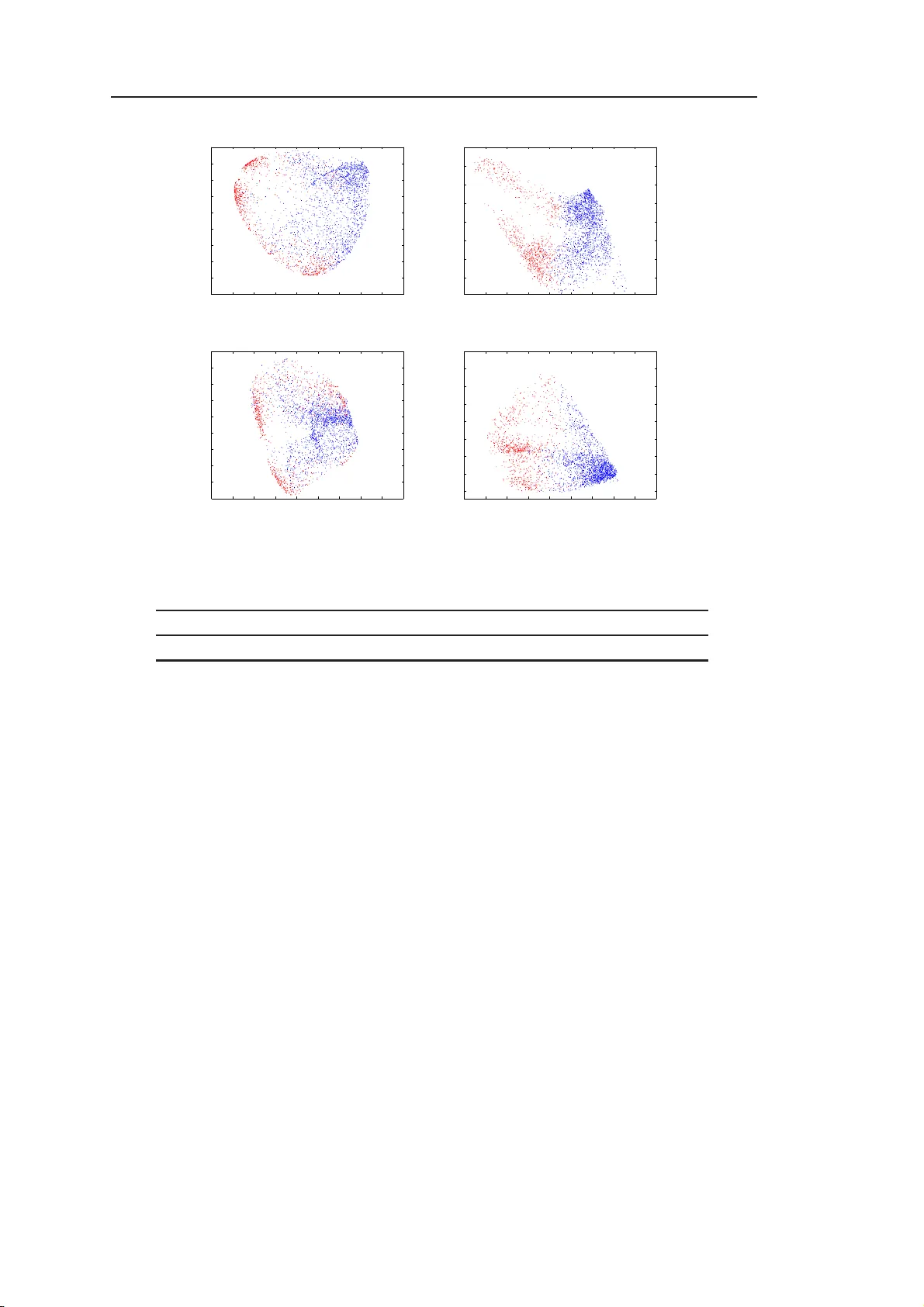
´ Ecole Do ctorale ED488 “Sciences, Ing ´ enierie, S ant ´ e” Sup ervised Metric Learning with Generalization Gu aran tees Th ` ese av ec lab el europ ´ een pr´ epar ´ ee par Aur ´ elien Bellet p our obtenir le grade de : Do cteur de l’Univ ersit ´ e Jean Monnet de Sain t- ´ Etienne Domaine : Informatique Lab orato ire Hub ert Curien, UMR CNRS 5516 F acult ´ e des Sciences et T ec hnique s Soutenance le 11 D ´ ece mbre 2012 au Lab oratoire Hub ert Cur ien dev an t le jury c omp os ´ e de : Pierre Dup on t Professeur, Univ ersit ´ e Catholique de Louv a in Rapp orteur R ´ emi Gilleron Professeur, Univ ersit ´ e de Lille Examinateur Amaury Habrard Professeur, Univ ersit ´ e d e Sain t- ´ Etienne Co-directeur Jose Oncina Professeur, Univ ersidad d e Alic ante Rapp orteur Liv a R alaivola Professeur, Aix-Marseille Univ ersit ´ e Examinateur Marc Sebban Professeur, Univ ersit ´ e de Sain t- ´ Etienne Directeur Remerciements Je tiens tout d’ab ord ` a remercier Pierre Dup on t, P rofesseur ` a l’Univ ersit´ e Catholique de Louv ain, et Jose O n cina, Professeur ` a l’Universit ´ e d’Alicant e, d ’a v oir accept ´ e d’ ˆ etre les rapp orteurs d e mon trav ail de th ` ese. Leurs r emarques p ertinente s m’on t p ermis d’am ´ eliorer la qualit ´ e de ce man uscrit. Plus g ´ en´ eralemen t, je remercie l’ensemble du jury , notammen t R ´ emi Gill eron, Professeur ` a l’Unive rsit´ e de Lille, et Liv a Ralaiv ol a, Professeur ` a Aix-Marseille Univ ersit ´ e, qui on t tout de suite a ccept ´ e d’ ˆ etre examinateurs. Je remercie c haleureusement mon directeur et mon co-directeur de th ` ese, Marc et Amaury , a v ec q u i j’ai d´ eve lopp´ e des liens pr ofessionn els et p e rsonn els qu i de toute ´ evidence dureront au-del` a de cette th ` ese. Je su is partic uli` erement reconnaissan t env ers Marc qui, malgr ´ e son attrait p ou r une certaine ´ equip e de f o ot ball, a su me conv aincre d e faire cette th ` ese et m’a fait conﬁance en acceptan t un arr angemen t extraordinaire (dans tous les sens du terme) p our qu e je p uisse passer ma premi` ere ann´ ee ` a ´ Edim b ourg. Je ve ux ´ egalemen t saluer les coll ` egues d u Lab oratoire Hub ert Curien et du d ´ epartement d’informatique de l’UJM. En premier lieu, mon voisin de bureau et ami JP , qui fut aussi un excellen t co- ´ equipier W arligh t. Je p ens e aus s i aux au tr es do ctoran ts (anciens et actuels) que son t Lauren t, Christophe, ´ Emilie, Da vid, F abien, T ung, C hahrazed et Mattias. Enﬁ n, je veux mentio nn er les p ersonnes r encon tr ´ ees dans le cadre des pro jets P ASCAL2 et LAMP AD A, notamment Emilie et Pierre du LIF de Marseill e a v ec qui j’esp ` ere av oir l’occasion d e trav ailler et de collab orer encore dans le futur. D’un p oint de vue p lu s p ersonnel, je salue ´ evidemment les amis, qui son t trop n om breux p our ˆ etre cit ´ es mais qui s e r econna ˆ ıtron t. L a pr´ esence d e certains ` a ma soutenance me fait ´ enorm ´ ement plaisir. Ces remerciements ne seraient p as complets sans un mot p our Marion, qui m’a b eaucoup soutenu et encourag ´ e p endan t ces (pr esqu e) trois ann ´ ees. Elle a mˆ eme essa y ´ e de s’in t´ eresser ` a la classiﬁcation lin ´ eaire parcimonieuse, r ´ eu ssissan t ` a faire illusion lors d’une r ´ eception ` a ECML! Enﬁn , last but not le ast , je d´ edie tout s implemen t cette th ` ese ` a mes parent s, mes grands-parents et mon p etit fr ` ere. iii Contents List of Figures vii List of T ables ix 1 In tro duction 1 I Bac kground 7 2 Preliminaries 9 2.1 Sup ervised Learn in g . . . . . . . . . . . . . . . . . . . . . . . . . . . . . . 9 2.2 Deriving Generalization Guarante es . . . . . . . . . . . . . . . . . . . . . 14 2.3 Metrics . . . . . . . . . . . . . . . . . . . . . . . . . . . . . . . . . . . . . 19 2.4 Conclusion . . . . . . . . . . . . . . . . . . . . . . . . . . . . . . . . . . . 27 3 A Review of Sup ervised Metric Learning 29 3.1 In tro d uction . . . . . . . . . . . . . . . . . . . . . . . . . . . . . . . . . . . 29 3.2 Metric Learning from F eature V ectors . . . . . . . . . . . . . . . . . . . . 30 3.3 Metric Learning from S tructured data . . . . . . . . . . . . . . . . . . . . 42 3.4 Conclusion . . . . . . . . . . . . . . . . . . . . . . . . . . . . . . . . . . . 45 I I Contributions in Metric Learning from Structured Data 49 4 A String Kernel Based on Learned E dit Similarities 51 4.1 In tro d uction . . . . . . . . . . . . . . . . . . . . . . . . . . . . . . . . . . . 51 4.2 A New Marginalized String E dit K ernel . . . . . . . . . . . . . . . . . . . 52 4.3 Computing the Edit Kernel . . . . . . . . . . . . . . . . . . . . . . . . . . 53 4.4 Exp erimental V alidation . . . . . . . . . . . . . . . . . . . . . . . . . . . . 59 4.5 Conclusion . . . . . . . . . . . . . . . . . . . . . . . . . . . . . . . . . . . 63 5 Learning Go o d Edit Similarities from Lo cal Constraints 65 5.1 In tro d uction . . . . . . . . . . . . . . . . . . . . . . . . . . . . . . . . . . . 65 5.2 The Theory of ( ǫ, γ , τ )-Goo d Similarit y F unctions . . . . . . . . . . . . . . 67 5.3 Preliminary Exp erimen tal Study . . . . . . . . . . . . . . . . . . . . . . . 71 5.4 Learning ( ǫ, γ , τ )-Go o d Edit S imilarit y F unctions . . . . . . . . . . . . . . 77 5.5 Theoretical Analysis . . . . . . . . . . . . . . . . . . . . . . . . . . . . . . 81 5.6 Exp erimental V alidation . . . . . . . . . . . . . . . . . . . . . . . . . . . . 89 5.7 Conclusion . . . . . . . . . . . . . . . . . . . . . . . . . . . . . . . . . . . 95 v vi CONTENTS I I I Con tributions in Metric Learnin g from F eature V ectors 99 6 Learning Go o d Bilinear Similarities from Global Constraints 101 6.1 In tro d uction . . . . . . . . . . . . . . . . . . . . . . . . . . . . . . . . . . . 101 6.2 Learning ( ǫ, γ , τ )-Go o d Bilinear S imilarit y F unctions . . . . . . . . . . . . 102 6.3 Theoretical Analysis . . . . . . . . . . . . . . . . . . . . . . . . . . . . . . 105 6.4 Exp erimental V alidation . . . . . . . . . . . . . . . . . . . . . . . . . . . . 109 6.5 Conclusion . . . . . . . . . . . . . . . . . . . . . . . . . . . . . . . . . . . 113 7 Robustness and Generalization for Metric Learning 117 7.1 In tro d uction . . . . . . . . . . . . . . . . . . . . . . . . . . . . . . . . . . . 117 7.2 Robustness and Generalizatio n for Metric Learning . . . . . . . . . . . . . 118 7.3 Necessit y of Robustness . . . . . . . . . . . . . . . . . . . . . . . . . . . . 124 7.4 Examples of R ob u st Metric Learning Algorithms . . . . . . . . . . . . . . 126 7.5 Conclusion . . . . . . . . . . . . . . . . . . . . . . . . . . . . . . . . . . . 129 8 Conclusion & P ersp ectives 131 List of Publications 135 A L earning Condit ional Edit Probabilities 137 B Pro ofs 141 B.1 Pro ofs of C h apter 5 . . . . . . . . . . . . . . . . . . . . . . . . . . . . . . 141 B.2 Pro ofs of C h apter 7 . . . . . . . . . . . . . . . . . . . . . . . . . . . . . . 147 Bibliograph y 153 List of Figures 1.1 The t w o-fold pr oblem of generalization in metric learning . . . . . . . . . 3 2.1 3D unit balls of th e L 1 , L 2 and L 2 , 1 norms . . . . . . . . . . . . . . . . . . 13 2.2 Geometric int erpr etation of L 2 and L 1 constrain ts . . . . . . . . . . . . . 13 2.3 Plot of s ev eral loss functions for binary classiﬁcation . . . . . . . . . . . . 14 2.4 Mink o wski distances: unit circles for v a rious v alues of p . . . . . . . . . . 22 2.5 Strategies to delete a n o de within a tree . . . . . . . . . . . . . . . . . . . 25 3.1 In tuition b ehind metric learning . . . . . . . . . . . . . . . . . . . . . . . 30 4.1 An example of m emoryless cPFT . . . . . . . . . . . . . . . . . . . . . . . 55 4.2 Tw o cPFT T | a and T | ab mo d eling p e ( s | a ) and p e ( s | ab ) . . . . . . . . . . . 56 4.3 The cPFT T | a and T | ab r epresen ted in the form of automata . . . . . . . 56 4.4 Automaton mo deling the in tersection of the automata of Figure 4.3 . . . . 57 4.5 A handwritten digit and its strin g repr esen tation . . . . . . . . . . . . . . 60 4.6 Comparison of our edit ke rn el with ed it d istances . . . . . . . . . . . . . . 61 4.7 Comparison of our edit ke rn el with other s tring kernels . . . . . . . . . . . 63 4.8 Inﬂuence of th e parameter t of K L & J . . . . . . . . . . . . . . . . . . . . . 64 5.1 A graphical insigh t in to ( ǫ, γ , τ )-go o dness . . . . . . . . . . . . . . . . . . 68 5.2 Pro jectio n space implied by the to y example of Figure 5.1 . . . . . . . . . 69 5.3 Estimation of the goo dness of edit similarities . . . . . . . . . . . . . . . . 72 5.4 Classiﬁcation accuracy and sparsit y (Digit dataset) . . . . . . . . . . . . . 74 5.5 Classiﬁcation accuracy and sparsit y with resp ect to λ . . . . . . . . . . . 75 5.6 Classiﬁcation accuracy and sparsit y with resp ect to t . . . . . . . . . . . . 75 5.7 Classiﬁcation accuracy and sparsit y (W ord dataset) . . . . . . . . . . . . . 76 5.8 Learning the edit costs: rate of con v ergence (W ord d ataset) . . . . . . . . 90 5.9 Inﬂuence of th e pairing s tr ategie s (W ord dataset) . . . . . . . . . . . . . . 91 5.10 Learning the separator: accuracy and sparsity results (W ord dataset) . . . 92 5.11 Learning the edit costs: rate of con v ergence (Digit dataset) . . . . . . . . 94 5.12 Inﬂ u ence of the pairing strategies (Digit dataset) . . . . . . . . . . . . . . 95 5.13 Example of a set of reasonable p oin ts (Digit dataset) . . . . . . . . . . . . 95 5.14 1-Nearest Neigh b or results (W ord dataset) . . . . . . . . . . . . . . . . . . 97 6.1 Accuracy of the metho ds with resp ect to KPC A d imension . . . . . . . . 112 6.2 F eature space induced b y the similarit y (Rings dataset) . . . . . . . . . . 113 6.3 F eature space induced b y the similarit y (Svmguide1 dataset) . . . . . . . 114 7.1 Illustration of robustness in th e classic and metric learning settings . . . . 120 vii List of T ables 1.1 Summary of notation . . . . . . . . . . . . . . . . . . . . . . . . . . . . . . 6 2.1 Common regularizers on v ectors . . . . . . . . . . . . . . . . . . . . . . . . 12 2.2 Common regularizers on matrices . . . . . . . . . . . . . . . . . . . . . . . 12 2.3 Example of an edit cost matrix . . . . . . . . . . . . . . . . . . . . . . . . 24 3.1 Metric learning from feature v ectors: main features of the metho ds . . . . 46 3.2 Metric learning from structured data: main features of th e metho ds . . . 46 4.1 Statistical comparison of our edit kernel with edit distances . . . . . . . . 61 4.2 Statistical comparison of our edit kernel with other strin g k ernels . . . . . 63 5.1 Example of a set of reasonable p o ints (W ord dataset) . . . . . . . . . . . . 92 5.2 Discriminativ e p atterns extracted from the reasonable p oints of T able 5.1 93 5.3 Summary of the main f eatures of GESL . . . . . . . . . . . . . . . . . . . 96 5.4 1-Nearest Neigh b or results on the Digit dataset . . . . . . . . . . . . . . . 97 6.1 Prop erties of the datasets used in the exp erim ental s tudy . . . . . . . . . 110 6.2 Accuracy of the linear classiﬁers bu ilt from the stud ied similarities . . . . 111 6.3 Accuracy of 3-NN classiﬁers us in g the stud ied similarities . . . . . . . . . 111 6.4 Runt ime of the studied metric learning metho ds . . . . . . . . . . . . . . 113 6.5 Summary of the main f eatures of SL LC . . . . . . . . . . . . . . . . . . . 114 ix “There is nothing more pr actical than a go o d theory .” — J ames C. Maxwel l “There is a theory whic h states that if eve r an yo ne disco v ers exactly what the Univ erse is for and why it is here, it w ill instant ly disapp ear and b e replaced by something even more bizarre and in exp licable. There is another theory which states that this has already h app ened.” — Douglas Ad ams xi CHAPTER 1 Intro duction The go al of mac hine learning is to automatica lly ﬁgure out ho w to perf orm ta sks by generalizing fr om examples. A mac hine learning algorithm tak es a d ata sample as inpu t and infers a mod el that captures the un derlying mec hanism (usu ally assumed to b e some unkn o wn probabilit y distribution) which generated the data. Data can consist of features v ectors (e.g., the age, b od y mass index, blo o d pressu re, ... of a patien t) or can b e s tr uctured, such as strings (e.g., text do c uments) or trees (e.g., XML do c uments). A classic setting is sup ervise d le arning , wher e the algorithm has access to a set of tr aining examples along with their lab els and m ust learn a mo del that is able to accurately predict the lab el of f uture (u nseen) exa mples. Sup ervised learning encompasses classiﬁcation problems, where the lab el set is ﬁnite (for in stance, predicting the lab el of a c haracter in a handwriting recognitio n system) a nd regression pr oblems, where the lab el set is con tin uous (for example, the temp erature in we ather forecasting). On the other hand, an unsup ervise d le arning algo rithm has no access to the lab e ls of the training data. A classic example is clustering, w here w e aim at assigning d ata in to similar group s . The generalizat ion abilit y of the learned mo del (i.e., its p erformance on un seen examples) can sometimes b e guaran teed using arguments from statistical learning theory . Relying on the sa ying “bir d s of a feather ﬂ o c k together”, many sup ervised and un su- p ervised mac h ine learning algorithms are based on a notion of metric (similarity or distance function) b et wee n examples, su c h as k -n earest neighbors or su pp o rt v ector ma- c hines in the sup ervised s etting and K -Mea ns clus terin g in unsu p ervised learning. The p erforman ce of these algorithms criticall y dep e nd s on the relev ance of the metric to the problem at hand — for instance, w e h op e that it identiﬁes as similar the examples th at share the same und erlying lab el and as dissimilar those of d iﬀeren t lab els. Unfortu- nately , stand ard metrics (suc h as the Eu clidean distance b etw een feature v ectors or th e edit distance b et wee n strin gs) are often not appropriate b ec ause th ey fail to capture the sp eciﬁc nature of the pr oblem of interest. F or this reaso n, a lot of eﬀort has gone into metric le arning , the r esearc h topic devot ed to automatica lly learning metrics fr om data. In this thesis, w e fo cus on sup ervised metric learning, where w e try to adapt the metric to the problem at hand using the informatio n brought by a sample of lab eled examples. Man y of these metho ds aim to ﬁ nd the parameters of a metric so that it b est satisﬁes a set of lo cal constrain ts o v er the training 1 2 Chapter 1. Introd uction sample, r equiring for instance that pairs of examples of the same class sh ould b e similar and that those of diﬀerent class s h ould b e dissimilar according to th e learned metric. A large b ody of w ork has b een dev oted to sup ervised m etric learning from feature ve ctors, in particular Mahalanobis distance learning, w h ic h essentia lly learns a linear pro jectio n of the d ata into a new sp ace where the local constraints are b ett er sat isﬁed. While early metho d s were costly and could n ot b e applied to m edium-sized problems, recen t metho ds oﬀer b etter scalabilit y and in teresting features such as sparsit y . Sup ervised metric learning from stru ctured data has receiv ed less attent ion b ecause it requires more complex pro cedures. Most of th e w ork has fo cused on learning metrics based on the edit distance. Roughly sp eaking, the edit distance b e t wee n t wo ob jects corresp onds to the c heap est sequence of edit op erations (ins ertion, d eletion and substitution of subparts) turning one ob ject in to the other, w here op er ations are assigned sp eciﬁc costs gathered in a m atrix. Edit distance learning consists in optimizing the cost matrix and u sually relies on maximizing the lik eliho o d of pairs of similar examples in a probabilistic m o del. Ov erall, w e id en tify t wo main limitatio ns of the curren t su p ervised metric learning meth- o ds. First, metrics are optimized b ased o n lo c al constraints and used in lo c al algorithms, in particular k -n earest neigh b ors. Ho we ve r, it is u nclear whether the s ame pro cedur es can b e used to obtain go o d metrics for u se in glob al algorithms such as linear separa- tors, whic h are simple y et p ow erful cla ssiﬁers that ofte n require less memory and pr o vide greater p rediction sp ee d than k -nea rest neigh b ors. In this con text, one ma y wan t to op- timize the metrics according to a glob al crite rion but, to the b est of our kno wledge, this has neve r b een addressed. Second, and p erh ap s more imp ortant ly , there is a substan- tial lac k o f theoret ical understanding of generalization in metric learning. It is w orth noting that in this con text, th e question of generalizati on is t wo-fold, as illustrated in Figure 1.1 . First, one ma y b e in terested in the generalization abilit y of the metric itself, i.e., its co nsistency not only on the training sample bu t also on unseen data co ming from the same distrib ution. V ery little wo rk has b een done on this matter, and existing framew orks lac k generali t y . Second, one ma y also b e in terested in the generalizat ion abilit y of the learning algorithm that uses the learned metric, i.e., can w e derive gener- alizati on guaran tees for the learned mo del in terms of the qualit y of the learned m etric? In practice, the learned metric is plugged into a learning algorithm and one can only hop e that it yields go o d results. Although some ap p roac hes optimize th e metric based on the decisio n rule of classiﬁcation algorithms su ch as k - nearest neigh b ors, this question has nev er b een in ve stigated in a formal wa y . As w e will see later in th is do cument, the recen tly-prop osed theory of ( ǫ, γ , τ )-goo d similarit y function ( Balcan et al. , 2008a , b ) has b een th e ﬁrst attempt to bridge the gap b etw een the prop er ties of a sim ilarity fun ction and its p e rform an ce in linear classiﬁcation, b u t h as n ot b een used so far in the con text of metric learning. This theory pla ys a central r ole in tw o of our con tributions. The limitations describ ed a b o v e constitute the main motiv ation for this thesis, and our co ntributions address them in sev eral wa ys. First, w e in tro du ce a string ke rn el Chapter 1. Introd uction 3 Metric learning algorithm Metric−based learning algorithm Learned metric Sample of examples Underlying unknown distribution Generalization guarantees for the learned model using the metric? Consistency guarantees for the learned metric? Learned model Sample of examples Figure 1.1: The t wo-fold problem o f gene r alization in metric lear ning. W e are in- terested in the g e ne r alization ability of the learned metr ic itself: can we s ay a nythin g ab out its cons is tency on unseen da ta drawn from the same distribution? F ur ther more, we are interested in the generaliza tio n ability of the learned mo del using that metric: can we relate its p e rformance on unse e n da ta to the qua lity of the learne d metr ic? that allo w s the u se of learned edit distances in k ernel-based methods su c h as supp ort v ector mac h ines. This pro vides a wa y to use these learned metrics in global classiﬁers. Second, w e prop ose t wo m etric learning ap p roac hes based on ( ǫ, γ , τ )-go o dness, for whic h generalizat ion guaran tees can b e deriv ed b oth for the learned metric itself and for a linear classiﬁer built from that metric. In the ﬁrst approac h (whic h deals with stru ctur ed data), the metric is optimized with resp ect to lo cal pairs to ensure the optimalit y of the solution. In th e second app roac h , dealing with f eature v ectors allo ws us to optimize a global criterion th at is m ore appropriate to linear classiﬁcation. Lastly , we introd uce a general framew ork th at c an be used to derive generalization guarantees for man y existing metric learning metho ds b ased on local constraint s. Con text of this w ork This th esis w as carried out in the mac hin e learning team of Lab oratoire Hub ert Cu r ien UMR CNRS 55 16, part of Univ ersit y of Sain t- ´ Etienne and Univ ersity of L y on. Th e con tribu tions presented in this thesis w ere dev elop e d in the context of the ANR pro ject Lampada 1 (ANR-09-EM ER-007), whic h deals w ith scaling learning algorithms to hand le large sets of s tr uctured data, with fo cuses on metric learning and sp arse learning, and P ASCAL2 2 , a Eur op ean Net work of Excellence supp orting researc h in mac hin e learnin g, statistics and optimization. Outline of the thesis This dissertation is organized as follo w s. P art I reviews the bac kground w ork relev ant to this thesis: • Ch apter 2 formally introdu ces the scien tiﬁ c conte xt: sup ervised learning, analytical framew orks for deriving generalizatio n guarante es, and v arious typ es of metrics. 1 http://lam pada.gforge.in ria.fr/ 2 http://pas callin2.ecs.so ton.ac.uk/ 4 Chapter 1. Introd uction • Ch apter 3 is a large survey of sup ervised metric learning from feature v ectors and structured data, with a fo cu s on th e relativ e merits and limitat ions of the metho ds of the literature. P art I I gathers our contributions on metric learning fr om structur ed d ata: • Ch apter 4 int ro d uces a n ew string k ernel based on learned edit pr obabilities. Unlik e other str ing edit k ernels, it is parameter-free an d guarante ed to b e v alid. Its n aiv e form requ ires the computation of an in ﬁnite su m o v er all ﬁnite strings that can b e bu ilt from the alphab e t. W e show ho w to g et roun d this problem b y using in tersection of pr obabilistic automata and algebraic manipulation. Exp eriments highligh t the p erform ance of our k ernel ag ainst state-of-t he-art string k ernels of the literature. • Ch apter 5 builds up on t he theory of ( ǫ, γ , τ )-go o d similarity function. W e ﬁr st sho w that w e can us e edit similarities directly in this framew ork and ac hieve competitiv e p erforman ce. The main con tribution of this c hapter is a n o v el m etho d for learning string and tree edit similarities called GESL (for Go o d Edit Similarit y Learning) that relies on a relaxed v ersion of ( ǫ, γ , τ )-goo d ness. The prop osed approac h, whic h is more ﬂexible than previous m etho ds, learn an edit simila rity from lo c al pairs and is then u sed to build a glob al linear classiﬁer. Using uniform stabilit y argument s, w e are able to derive generaliza tion g uarantee s for th e learned similarit y that actually give an upp er b ound on t he ge neralization error of th e linear classiﬁer. W e conduct extensiv e exp erimen ts that show the usefu lness of ou r app roac h and the p erform an ce and sp arsit y of the resulting linear classiﬁers. P art I I I gathers our con tributions on metric learning from feature vec tors: • Ch apter 6 presents a new b ilinear similarit y learning metho d for linear classiﬁca- tion, calle d SLLC (for Similarit y L earn ing for Linear C lassiﬁcation). Unlik e GESL, SLLC directly optimize s the empirical ( ǫ, γ , τ )-go o dness criterion, whic h m akes the approac h en tirely glob al : the similarit y is optimized with r esp ect to a global cri- terion (instea d of lo cal pairs) a nd plugged in a global linear classiﬁer. S LLC is form ulated as a con ve x minimization problem that can b e eﬃcien tly sol ve d in a batc h or online wa y . W e also k ernelize our approac h, thus learning a linear s im i- larit y in a nonlin ear feature sp ace induced by a k ernel. Using similar arguments as f or GESL, we deriv e generalization guaran tees for SLLC h ighligh ting that our metho d actually min im izes a tight er b ound on the generalizatio n error of the clas- siﬁer than GESL. Exper im ents on sev eral stand ard datasets sho w that SLLC leads to comp etit ive classiﬁers that ha v e the additional adv an tage of b eing v ery s parse, th us sp e eding up prediction. Chapter 1. Introd uction 5 • Ch apter 7 ad d resses the lack of general framew ork for establishing generalization guaran tees for metric learning. It is based on a sim p le adaptation of algorithmic robustness to the case where training data is made of pairs of examples. W e sho w that a r obust metric learning algorithm has generalization guaran tees, and furthermore that a wea k n otion of r obustness is actually necessary and suﬃcien t for a metric learning algorithm to generalize. W e illustrate the usefulness of our approac h b y sho wing that a large class of m etric learning algorithms are robu st. In particular, w e a re a ble to deal with sparsity-i nd ucing regularizers, whic h w as not p ossible with previous framew orks. Notation Throughout this do cument, N denotes th e s et of natural n umb er s while R and R + resp ectiv ely denote th e sets of real num b ers a nd nonnegativ e real num b e rs. Arbitrary sets are denoted b y calligraphic letters suc h as S , a nd |S | stand s for the n umb er of elemen ts in S . A set of m elemen ts f rom S is denoted by S m . W e denote v ectors b y b old lo w er case letters. F or a v ector x ∈ R d and i ∈ [ d ] = { 1 , . . . , d } , x i denotes the i th comp onent of x . The inner p r o duct b et w een tw o v ectors is denoted b y h· , ·i . W e denote matrices by b old u pp e r case letters. F or a c × d real-v alued matrix M ∈ R c × d and a p air of integ ers ( i, j ) ∈ [ c ] × [ d ], M i,j denotes the en try at ro w i and column j of the matrix M . The identit y m atrix is denoted b y I and the cone of symmetric p ositi ve semi-deﬁnite (PSD) d × d real-v alued matrices b y S d + . k · k denotes an arbitrary (v ector or m atrix) norm and k · k p the L p norm. Strings are d enoted b y sans serif letters suc h as x . W e u s e | x | to denote the length of x and x i to r efer to its i th sym b o l. In the conte xt of learning problems, w e use X a nd Y to denote th e inp ut space ( or instance space) and the output space (or label space) resp ectiv ely . W e use Z = X × Y to denote th e join t space, and an arb itrary lab eled instance is denoted by z = ( x, y ) ∈ Z . The hinge function [ · ] + : R → R + is deﬁned as [ c ] + = max(0 , c ). Pr[ A ] denotes the probabilit y of the even t A , E [ X ] the exp ectation of the random v ariable X and x ∼ P indicates that x is dr a wn according to the probability distribu tion P . A su mmary of the n otations is giv en in T able 1.1 . 6 Chapter 1. Introd uction Notation Description R Set of real n umbers R + Set of nonnegativ e real num b ers R d Set of d -dimensional real-v alued vectors R c × d Set of c × d real-v alued matrices N Set of natural n umbers, i.e., { 0 , 1 , . . . } S d + Cone of symmetric PSD d × d real-v alued matrices [ k ] The set { 1 , 2 , . . . , k } S An arbitrary set |S | Number of elemen ts in S S m A set of m elements from S X Input space Y Output space z = ( x, y ) ∈ X × Y An arbitrary labeled instance x An arbitrary v ector x j , x i,j The j th compon ent of x and x i h· , ·i Inner product b etw een vectors [ · ] + Hinge function M An arbitrary matrix I The iden tity matrix M i,j Entry at row i and column j of matrix M k · k An arbitrary norm k · k p L p norm x An arbitrary string | x | Length of string x x i , x i , j j th symbol of x and x i x ∼ P x is dra wn i.i.d. from probability d istribu tion P Pr[ · ] Probabilit y of even t E [ · ] Exp ectation of random v ariable T able 1. 1: Summary of notation. P AR T I Background 7 CHAPTER 2 Prelimi na r ies Chapter abstract In this c ha pter, we intro duce the sc ie nt iﬁc context of this th esis a s well as r elev ant bac kgr ound work. W e ﬁrst intro duce forma lly the sup ervised learning setting and describ e the main idea s of statistica l learning theory , with a focus on bi- nary class iﬁcation. W e then presen t three analytica l frameworks (uniform con vergence, uniform stability and a lgorithmic robustness) for establishing that a learning algo rithm has g eneralizatio n guar antees. Lastly , we recall the deﬁnitio n o f several t y pes of metrics and give examples of such functions fo r feature vectors and structured data. 2.1 Sup ervised Learning The goal of sup erv ised learning 1 is to automaticall y infer a mo del (h yp o thesis) from a set of labeled examples t hat is a ble to mak e predictions give n n ew un lab eled data . In the follo wing, w e review basic notions of statistical learning theory , a v ery p opular framew ork p ioneered b y V apnik & Chervo nenkis ( 1971 ). Th e in terested r eader can refer to V apnik ( 1998 ) and Bousquet et al. ( 2003 ) for a m ore thorough d escription. 2.1.1 T ypical Se tt ing In su p ervised learning, we learn a h yp othesis from a s et of labeled examples. T his notion of training samp le is formalized b elo w. Deﬁnition 2.1 (T rainin g sample) . A training sample of size n is a set T = { z i = ( x i , y i ) } n i =1 of n observ ations indep e nd en tly and iden tically distributed (i.i.d.) according to an u nknown j oin t distribution P ov er the sp ace Z = X × Y , where X is the input space an d Y the output sp ace. F or a give n observ ation z i , x i ∈ X is the instance (or example) and y i ∈ Y its lab e l. When Y is discrete, w e are dealing with a classiﬁcation task, and y i is called the class of x i . When Y is con tinuous, this is a regression task. In this t hesis, w e mainly fo c us on binary cla ssiﬁcation tasks, where we assume Y = {− 1 , 1 } . 1 Note that there exist other learning paradigms , such as unsup ervised lea rning ( Ghahramani , 20 03 ), semi-sup ervised learning ( Chapelle et al. , 2006 ), transfer learning ( Pan & Y ang , 2010 ), reinforcemen t learning ( Sutton & Barto , 1998 ), etc. 9 10 Chapter 2. Preliminaries W e will mostly deal with feature vec tors and strings. F or feature v ectors, we generally assume that X ⊆ R d . F or strings, w e need the follo wing deﬁnition. Deﬁnition 2.2 (Alphab et and string) . An alphab et Σ is a ﬁnite nonempty set of sym- b ols. A string x is a ﬁ nite sequ ence of symb ols from Σ. The empty string/sym b ol is denoted b y $ and Σ ∗ is the set of all ﬁnite strings (including $) that can b e generated from Σ. Finally , the length of a string x is denoted b y | x | . W e can n ow form ally deﬁn e wh at we mean by sup ervised learnin g. Deﬁnition 2.3 (Sup ervised learning) . Sup ervised learning is the ta sk of inferr ing a function (often r eferred to as a h yp o thesis or a mo d el) h T : X → L b elonging to some h yp ot hesis class H f rom a training sample T , whic h “best” predicts y from x for an y ( x, y ) d r a wn from P . No te that the decision space L m a y or ma y not b e equal to Y . In ord er to c ho ose h T , w e need a criterion to assess the qualit y of an arbitrary hyp othesis h . Giv en a nonnegativ e loss function ℓ : H × Z → R + measuring the degree of a greemen t b et wee n h ( x ) and y , we d eﬁne the notion of true risk. Deﬁnition 2 .4 (T rue risk) . The true risk (also called generalizatio n error) R ℓ ( h ) of a h yp ot hesis h with r esp ect to a loss fun ction ℓ is th e exp ected loss suﬀered by h o v er the distribution P : R ℓ ( h ) = E z ∼ P [ ℓ ( h, z )] . The most natural loss function for bin ary classiﬁcation is the 0/1 loss (also called clas- siﬁcation error): ℓ 0 / 1 ( h, z ) = ( 1 if y h ( x ) < 0 0 otherwise . R ℓ 0 / 1 ( h ) then co rresp onds to the prop ortion of time h ( x ) and y agree in sign, and in particular to the pr op ortion of correct p redictions w h en L = Y . The goal of sup ervised learning is then to ﬁn d a hyp othesis that ac hiev es the smallest true risk. Unfortunately , in general we cannot compute the true risk of a h y p othesis since the distribu tion P is un kno wn. W e can only measure it empirically on the training sample. This is called th e emp irical r isk. Deﬁnition 2.5 (Empirical risk ) . Let T = { z i = ( x i , y i ) } n i =1 b e a training sample. The empirical risk (also called emp irical error) R ℓ T ( h ) of a h yp othesis h o ve r T with resp ect to a loss fu nction ℓ is the a v erage loss su ﬀered by h on the instances in T : R ℓ T ( h ) = 1 n n X i =1 ℓ ( h, z i ) . Chapter 2. Preliminaries 11 Under some restrictions, u sing the emp ir ical risk to select the b est hyp othesis is a go o d strategy , as d iscussed in the next section. 2.1.2 Finding a Goo d Hyp othesis This section fo cuses on classic strategies for ﬁn ding a go o d hyp othesis in the true risk sense. The d eriv ation of guarantee s on the true r isk of the selected hyp othesis will b e studied in Section 2.2 . Simply minimizing the empirical risk o ver all p ossible hyp otheses wo uld ob viously b e a go o d strategy if inﬁnitely many training instances were a v ailable. Unfortunately , in real istic scenarios, trainin g data is limited and there alw ays e xists a h yp othesis h , ho w ev er complex, that p erfectly p r edicts the training samp le, i.e., R ℓ T ( h ) = 0 , but generalizes p o orly , i.e., h has a n onzero (p otent ially large) true risk. This situation wh ere the true r isk of a hypothesis is m uch larger than its empirical risk is called overﬁtting . The intuitiv e idea behin d it is that learnin g the training sample “b y h eart” do e s not pro vide go o d generalization to unseen data. There is therefore a trade-oﬀ b et w een min im izing the empirical risk and the complexit y of the consider ed h yp ot heses, kno wn as the bias-v ariance trade-oﬀ. Th ere essentially exist t w o wa ys to deal w ith it and a v oid ov erﬁtting: (i) restrict the h yp othesis space, and (ii) fa v or simple hyp otheses o ve r complex ones. In the follo win g, w e brieﬂy presen t three classic str ategies for ﬁ n ding a hyp othesis with small true risk. Empirical Risk Minimization The idea of the Empirical Risk Minimization (ERM) principle is to pic k a restricted hypothesis space H ⊂ L X (for in stance, linear classiﬁers, decision trees, etc.) and select a hyp othesis h T ∈ H that minimizes the empir ical risk: h T = arg min h ∈H R ℓ T ( h ) . This m a y w ork well in p ractice b ut dep ends on the choice of h yp othesis space. E s - sen tially , we w ant H large enough to include h yp otheses with small risk, but H small enough to a void o verﬁtting. Without bac kground knowledge on the t ask, pic king an appropriate H is diﬃcult. Structural Risk Minimization In Structural Risk Minimization (SRM), w e u se an inﬁnite sequence of hyp othesis classes H 1 ⊂ H 2 ⊂ . . . of increasing size an d s elect the h yp ot hesis that minim izes a p enalized v ersion of th e empir ical risk that fav ors “simple” classes: h T = arg min h ∈H c ,c ∈ N R ℓ T ( h ) + pen ( H c ) . 12 Chapter 2. Preliminaries Name F ormula Pros Cons L 0 norm k x k 0 Number of nonzero components SP N CO, NSM L 1 norm k x k 1 P | x i | CO, SP NSM (Squared) L 2 norm k x k 2 2 P x 2 i CO, SM L 2 , 1 norm k x k 2 , 1 Sum of L 2 norms of grouped v ariables CO, GSP NSM T able 2.1: Commo n r egularizer s on vectors. CO/NCO sta nd for conv ex /nonconv ex, SM/NSM for smo o th/nonsmo oth and SP/ GSP for s pa rsity/group sparsity . Name F ormula Pros Cons L 0 norm k M k 0 Number of nonzero components SP N CO, NSM L 1 norm k M k 1 P | M i,j | CO, SP N SM (Squared) F roben ius norm k M k 2 F P M 2 i,j CO, SM L 2 , 1 norm k M k 2 , 1 Sum of L 2 norms of ro ws/columns CO, GSP NSM T race (nuclear) norm k M k ∗ Sum of singular v alues CO, LO NSM T able 2.2: Common regula rizers on matrice s . Abbreviations are the same as in T able 2.1 , with LO standing for low-rank. This imp lemen ts the Occam’s r azor p rinciple according to wh ich one should choose th e simplest explanation consisten t with the training data. Regularized Risk Minimization Regularize d Risk Minimiza tion (RRM) also builds up on the Occam’s razor principle bu t is easier to implement: one p icks a single, large h yp ot hesis space H and a regularizer (usually some norm k h k ) and selects a hyp othesis that ac h iev es the b est trade-oﬀ b et wee n empirical risk minimization and r egularizatio n: h T = arg m in h ∈H R ℓ T ( h ) + λ k h k , (2.1) where λ is the trade-oﬀ parameter (in practice , it is set using v alidation data). The role of r egularization is to p enalize “complex” hypotheses. Note that it also pro vides a built-in w a y to br eak the tie b et wee n hyp otheses th at h a v e the same empirical risk. The c hoice of regularizer is im p ortan t and dep ends on the considered task and the desired eﬀect. Common regularizers for v ector and matrix m o dels are giv en in T able 2.1 and T able 2 .2 resp ectiv ely . Some regularizers are easy to optimize b eca use they are con v ex and smo oth (for instance, the squ ared L 2 norm) while others do not ha ve these con v enien t p rop erties and are thus harder to deal with (see Figure 2.1 for a graphical insigh t into some of these r egularizers). Ho wev er, the latter ma y bring some p ote ntia lly in teresting eﬀects suc h as sparsity: they tend to set some p arameters of the hyp othesis to zero. Figure 2.2 illustrates this on L 2 and L 1 constrain ts — this also holds for regularization. 2 2 In fact, regularized and constrained problems are equiv alent in the se nse that for any v alue of the parameter β of a feasible co nstrained problem, there exists a v alue of the parameter λ of t he Chapter 2. Preliminaries 13 Figure 2.1: 3D unit balls of the L 1 , L 2 and L 2 , 1 norms (ta ken from Grandv ale t , 2011 ). The L 2 norm is conv ex, smo oth and do es not induce sparsity . The L 1 norm is co nvex, nonsmo oth and induces sparsity at the co o rdinate level. The L 2 , 1 norm is conv ex, nonsmo o th a nd induces spa rsity at the gr o up level (simultaneous spa rsity of co ordinates b elo nging to the sa me predeﬁned group). L 1 constrain t L 2 constrain t Figure 2 .2: Geometric interpretation of L 2 and L 1 constraints in 2D. Suppo se that we a re lo oking f or a hypothesis h ∈ R 2 with a constraint k h k ≤ β (represe nt ed in dark blue) tha t minimizes the empirical r isk (represented by the lig ht gre e n cont our line). U nlike the L 2 norm, the L 1 norm tends to zero out co ordinates, th us reducing dimensionality . Regularizatio n is used in many successful learning metho ds and, as w e will see in Sec- tion 2.2 , ma y help deriving generaliza tion guaran tees. 2.1.3 Surrogate Loss F unctions The metho d s d escrib ed ab o ve all rely on m inimizing the emp irical risk . Ho we ve r, due to the n on conv exit y of the 0/1 loss, minimizing (or app ro ximately min imizing) R ℓ 0 / 1 is kno wn to b e NP-hard ev en for simple hypothesis classes ( Ben-Da vid et al. , 2003 ). F or this r eason, surrogate conv ex loss fun ctions (that can b e m ore eﬃcien tly h andled) are often used. The most p rominent choic es in the conte xt of b inary classiﬁcation are: • the hinge loss: ℓ hing e ( h, z ) = [1 − y h ( x )] + = max(0 , 1 − y h ( x )), used for instance in supp o rt vecto r mac h ines ( Cortes & V apn ik , 1995 ). • the exp onen tial loss: ℓ exp ( h, z ) = e − y h ( x ) , used in Adab oost ( F reund & Schapire , 1995 ) . correspondin g regularized problem such that b oth p roblems have th e same set of solutions, and vice versa . In practice, regulari zed problems are more con venien t to use because they are alw a ys feasible. 14 Chapter 2. Preliminaries -0.5 0 0.5 1 1.5 2 2.5 3 3.5 -2 -1.5 -1 -0.5 0 0.5 1 1.5 2 Classiﬁcation error (0/1 loss) Hinge loss Logistic loss Exp onential loss y h ( x ) ℓ ( h, z ) Figure 2.3: Plot of several loss functions for binary c lassiﬁcation. • the logistic loss: ℓ log ( h, z ) = log(1 + ǫ − y h ( x ) ), used in Logitb o ost ( F riedman et al. , 2000 ) . These loss f unctions are plotted in Figure 2.3 along with the n oncon v ex 0/1 loss. Cho osing an appropriate loss fun ction is not an easy task and strongly dep ends on the problem, but there exist general results on the r elativ e merits of diﬀerent loss fu nctions. F or in stance, Rosasco et al. ( 2004 ) studied statistical prop erties of several conv ex loss functions in a general classiﬁcation setti ng and concluded that the hinge loss h as a better con v ergence r ate than other loss f u nctions. Ben-Da vid et al. ( 2012 ) ha ve fu rther sho wn that in the con text of linear classiﬁcation, the hin ge loss oﬀers the b e st guaran tees in terms of classiﬁcation err or. In the follo wing section, we present analytical fr amew orks that allo w the deriv ation of generalizat ion guaran tees, i.e., relating the empirical risk of h T to its tr u e r isk. 2.2 Deriving Generalization Guaran tees In the previous sec tion, w e describ ed a few generic metho ds for learning a h yp othesis h T from a training sample T based on minimizing the (p enaliz ed) emp irical risk. Ho wev er, learning a hyp othesis with small true risk is wh at we are r eally int erested in. Typically , the empirical risk can b e seen as an optimisticall y biased esti mation of the true risk (esp ecially when the training sample is small), and a considerable amount of researc h has gone into deriving generaliza tion guaran tees for learning algorithms, i.e., b ound ing the deviation of the true r isk of the learned hyp othesis from its empirical measurement. These b ound s are often referred to as P A C (Pr obably Appro ximately Correct) b oun ds Chapter 2. Preliminaries 15 ( V aliant , 1984 ) and ha v e the follo wing form: Pr[ | R ℓ ( h ) − R ℓ T ( h ) | > ǫ ] ≤ δ , where ǫ ≥ 0 and δ ∈ [0 , 1]. In other w ords, it b ound s the probabilit y to observ e a large gap b et we en the true risk and the empirical risk of an hyp othesis. The k ey instruments for deriving P A C b ounds are concen tration inequ alities. They es- sen tially assess the deviation of s ome fu nctions of ind ep endent r andom v ariables from their exp ectation. Diﬀerent concen tration inequ alities tac kle diﬀeren t fu n ctions of the v ariables. The most commonly u sed in m ac h ine learning are C heb yshev (only one v ari- able is considered), Ho eﬀding (sums of v ariables) and McDiarmid (that can accommo- date any suﬃciently regular fu nction of the v ariables). F or more d etails ab out concen- tration inequalities, see f or in s tance th e su rve y of Bouc h eron et al. ( 2004 ). In this section, w e presen t three theoretical framewo rks for establishing generalizatio n b ound s: uniform conv ergence, u niform s tability and algorithmic robustn ess (for a more general o verview, please r efer to the tu torial by Langford , 2005 ). Note that our con tr i- butions in Chapter 5 , Chapter 6 and Chapter 7 m ak e use of th ese framew orks. 2.2.1 Uniform Conv ergence The theory of uniform con ve rgence of empirical qu an tities to their mean ( V apnik & Chervo nenkis , 1971 ; V apnik , 1982 ) is one of the most pr ominen t to ols for deriving gen- eralizatio n b ounds. It p ro vides guaran tees that hold f or any hyp othesis h ∈ H (including h T ) and essentially b ounds (with some probabilit y 1 − δ ) the true risk of h by its em- pirical risk p lus a p enal ty term that dep end s on the num b er of training examples n , the size (or complexity) of the hyp othesis space H and the v alue of δ . Intuitiv ely , large n brings high conﬁdence (sin ce as n → ∞ the empirical r isk conv erges to the tru e risk by the la w o f large n umb ers), complex H brings low conﬁ d ence (since o v erﬁtting is more lik ely), and δ accoun ts for the probabilit y of dra wing an “unluc ky” training sample (i.e., not represent ativ e of the und erlying distribu tion P ). When the h yp othesis space is ﬁnite, w e get the follo wing P AC b ound in O (1 / √ n ). Theorem 2.6 (Uniform conv ergence b ound for the ﬁn ite case) . L et T b e a tr aining sample of size n dr awn i.i.d. fr om some distribution P , H a ﬁnite hyp othesis sp ac e and δ > 0 . F or any h ∈ H , with pr ob ability 1 − δ over the r andom sample T , we have: R ℓ ( h ) ≤ R ℓ T ( h ) + r ln |H | + ln(1 /δ ) 2 n . When H is co ntin uous (for instance, if H is th e space of linear classiﬁers), w e n eed a measure of the complexit y of H such as the V C dimension ( V apnik & Ch erv onenkis , 16 Chapter 2. Preliminaries 1971 ) , the fat-shattering dimension ( Alon et al. , 1997 ) or th e Rademac her c omplexit y ( Koltc h in skii , 200 1 ; Bartlett & Me nd elson , 2002 ). F or instance, using the VC dimension, w e get the follo wing b ound . Theorem 2.7 (Uniform con v ergence b ound with V C d imension) . L et T b e a tr aining sample of size n dr awn i.i.d. fr om some distribution P , H a c ontinuous hyp othesis sp ac e with VC dimension V C ( H ) and δ > 0 . F or any h ∈ H , with pr ob ability 1 − δ over the r andom sample T , we have: R ℓ ( h ) ≤ R ℓ T ( h ) + v u u t V C ( H )  ln 2 n V C ( H ) + 1  + ln(4 /δ ) n . A dra wb ack of un iform con v ergence analysis is that it is only based on the size of the training sample and the complexit y of the h yp othesis space, and completely ignores the learnin g alg orithm, i.e., ho w the h yp othesis h T is s elected. 3 In the follo wing, w e present tw o an alytical frameworks that explicitly tak e into accoun t the algorithm and can b e used to deriv e generalization guarantee s f or h T sp eciﬁcally , in particular in the regularized risk minimization setting ( 2.1 ). 2.2.2 Uniform Stability Building on pr evious w ork on algorithmic stabilit y , Bousquet & Elissee ﬀ ( 20 01 , 200 2 ) in tro du ced new deﬁ n itions that allo w the deriv ation of generalization b oun ds for a large class o f algorithms. In tuitiv ely , an algorithm is said stable if it is robu st to small c hanges in its in p ut (in our case, the trainin g samp le), i.e., the v ariation in its outpu t is small. F ormally , w e fo cus on un iform stabilit y , a ve rsion of stabilit y that allo ws the deriv ation of rather tigh t b ounds. Deﬁnition 2.8 (Uniform stabilit y) . An al gorithm A has u niform stabilit y κ/n with resp ect to a loss fu nction ℓ if the follo w ing holds: ∀T , |T | = n , ∀ i ∈ [ n ] : sup z | ℓ ( h T , z ) − ℓ ( h T i , z ) | ≤ κ n , where κ is a p o sitiv e constan t, T i is obtained from the training sample T by r eplacing the i th example z i ∈ T b y another example z ′ i dra wn i.i.d. from P , h T and h T i are the h yp ot heses learned by A from T and T i resp ectiv ely . 4 3 In fact, the Rademacher complexit y can sometimes implicitly take into account t h e regularization term of the al gorithm. 4 Deﬁnition 2.8 corresp onds to t he case where th e training sample is altered through the replacement of an instance by another. Bousquet & Elisseeﬀ ( 2001 , 2002 ) also give a deﬁnition of uniform stabilit y based on th e remo v al of an instance from the training sample, which implies Deﬁn ition 2.8 . W e will use Deﬁnition 2.8 throughout this thesis: w e ﬁnd it more con venien t to deal with since replacemen t preserves th e size of t he training sample. Chapter 2. Preliminaries 17 Bousquet & Elisseeﬀ ( 2001 , 2002 ) ha v e sho wn that a large class of regularized r isk minimization algorithms sat isﬁes this deﬁnition. Th e constan t κ t yp ically dep ends on the form o f the loss function, the regularizer an d the regularization p arameter λ . Making a go o d us e of Mc Diarmid’s inequalit y , they show that wh en Deﬁn ition 2.8 is fulﬁ lled, the follo win g b ound in O (1 / √ n ) h olds. Theorem 2.9 (Uniform stabilit y b o un d) . L et T b e a tr aining sample of size n dr awn i.i.d. fr om some distribution P and δ > 0 . F or any algorithm A with uniform stability κ/n with r e sp e ct to a loss function ℓ upp er-b ounde d by some c onstant B , 5 with pr ob ability 1 − δ over the r andom sample T , we have: R ℓ ( h T ) ≤ R ℓ T ( h T ) + κ n + (2 κ + B ) r ln(1 /δ ) 2 n , wher e h T is the hyp othesis le arne d by A fr om T . The main d iﬀerence b et w een un iform con ve rgence and u niform stabilit y is that the lat- ter incorp orates r egularizatio n (through κ and h T ) and do es not r equire an y hyp othesis space complexit y argument. In particular, uniform stabilit y can b e u s ed to d eriv e gen- eralizatio n guaran tees for hypothesis classes that are diﬃcult to analyze with classic complexit y argumen ts, s uc h as k -nearest neigh b ors or supp ort ve ctor machines that ha v e inﬁnite VC dimension. I t can also b e adapted to n on-i.i.d. settings ( Mohri & Rostamizadeh , 2007 , 2010 ). W e will u se uniform stabilit y in the con tributions presented in Chapter 5 and Chap ter 6 . On the other hand, Xu et al. ( 20 12a ) ha v e shown that a lgorithms with sp ars it y -in d ucing regularization are not stable. 6 Algorithmic robustness, presented in the next section, is able to d eal w ith su c h algorithms. W e will mak e use of this framew ork in Chapter 7 . 2.2.3 Algorithmic R obustness Algorithmic robustness ( Xu & Mannor , 2010 , 2012 ) is the abilit y of an algorithm to p erform “similarly” on a tr aining example and on a test example that are “close”. It relies on a p artitioning of the space Z to charact erize closeness: t w o examples are close to eac h other if they lie in th e same partition of the sp ace. The partition itself is based on th e n otion of co v ering num b er ( Kolmogoro v & Tikh omiro v , 1961 ). Deﬁnition 2.10 (Co v ering n umb er ) . F or a metric s p ace ( S , ρ ) and V ⊂ S , we say that ˆ V ⊂ V is a γ -co v er of V if ∀ t ∈ V , ∃ ˆ t ∈ ˆ V suc h th at ρ ( t, ˆ t ) ≤ γ . The γ -co v ering num b er of V is N ( γ , V , ρ ) = min n | ˆ V | : ˆ V is a γ -co ver of V o . 5 Note that many loss functions are unb ounded if their domain is assumed to b e unboun ded ( see Figure 2.3 ), but in practice t h ey hav e b ound ed domain due for example to the common assumption that the norm of an y instance is boun ded. 6 Sparsity is seen here as the abilit y to identify redundan t features. 18 Chapter 2. Preliminaries In particular, wh en X is compact, N ( γ , X , ρ ) is ﬁn ite, leading to a ﬁnite co ver. Then, Z can b e partitioned in to |Y |N ( γ , X , ρ ) subsets s u c h that if tw o examples z = ( x, y ) and z ′ = ( x ′ , y ′ ) b elong to the same subset, then y = y ′ and ρ ( x, x ′ ) ≤ γ . W e can n ow form ally deﬁn e the n otion of robustness. Deﬁnition 2.11 (Algorithmic r ob u stness) . Algorithm A is ( K , ǫ ( · ))-robust, for K ∈ N and ǫ ( · ) : Z n → R , if Z can b e partitioned in to K disjoin t s ets, denoted b y { C i } K i =1 , suc h that the follo w in g holds for all T ∈ Z n : ∀ z ∈ T , ∀ z ′ ∈ Z , ∀ i ∈ [ K ] : if z , z ′ ∈ C i , then | ℓ ( h T , z ) − ℓ ( h T , z ′ ) | ≤ ǫ ( T ) , where h T is the hyp othesis learned by A from T . Brieﬂy s p eaking, an algorithm is robust if for an y example z ′ falling in the same sub set as a training example z , then the gap b etw een the losses asso ciated with z and z ′ is b ound ed (b y a qu an tit y that ma y dep end on the trainin g sample T ). T he existence of the partition itself is guaran teed by the deﬁnition of co vering n umb er . No te that b o th uniform s tability and algorithmic robus tness prop erties in v olv e a b ound on deviations b et wee n losses. The key d iﬀerence is th at uniform stabilit y studies the v ariation of the loss associated with a ny example z u n der sm all c hanges in the training sample (implying that the le arned h y p othesis itself do es not v ary muc h ), while algorithmic robustness considers the deviation b e tw een the losses asso ciated with t w o examples that are close (implying that the learned h yp othesis is lo cally consisten t). Xu & Mannor ( 2010 , 2012 ) hav e sho wn that a robust algorithm has generalization guar- an tees. Th is is formalized by the follo w in g theorem. Theorem 2 .12 (Robustness b ound) . L e t ℓ b e a loss function upp er-b ounde d by some c onstant B , and δ > 0 . If an algorithm A is ( K , ǫ ( · )) -r obust, then with pr ob ability 1 − δ , we have: R ℓ ( h T ) ≤ R ℓ T ( h T ) + ǫ ( T ) + B r 2 K ln 2 + 2 ln(1 /δ ) n , wher e h T is the hyp othesis le arne d by A fr om T . Note that ther e is a tradeoﬀ b et w een the size K of the partition and ǫ ( T ): the latter can essen tially b e made as small as p ossible by us in g a ﬁn er-grained cov er. P A C b ounds based on robustness are generally n ot tig ht since they r ely on uns p ec- iﬁed (p ote ntia lly large) co vering n umb ers. On the o ther hand, a great adv anta ge of robustness is that it can deal with a larger class of regularizers than stabilit y (in p artic- ular, sparsit y -in d ucing norms can b e consid er ed ), and its geometric in terpretation mak es adaptations to non -stand ard settings (su c h as non-i.i.d. data) p ossib le. Our contribu- tion in Chapter 7 adapts robustness to the case of metric learning, when trainin g data consist of non -i.i.d. pairs of examples. Finally , note that Xu & Mannor ( 2010 , 2 012 ) Chapter 2. Preliminaries 19 established that a we ak notion of robustness is n ecessary and su ﬃcien t f or an algorithm to generalize asymptotically , making robustness a key prop erty for th e generalizatio n of learning algorithms. After ha ving presente d the su p ervised learning setting and analytica l f ramew orks for deriving generaliza tion guaran tees, w e no w turn to th e topic of m etrics, whic h has a great place in this thesis. 2.3 Metrics The notion of metric (us ed here as a generic term for distance, similarit y or dissim- ilarit y function) pla ys an imp ortant role in man y mac hine learning problems suc h as classiﬁcation, regression, clustering, or ranking. Successful examples include: • k -Nearest Neigh b ors ( k -NN) classiﬁcat ion ( Co v er & Hart , 196 7 ), where the p re- dicted cla ss of an instance x corresp onds to the ma jorit y class among the k -nearest neigh b ors of x in the training samp le, according to some distance or similarit y . • Kern el metho ds ( Sc h¨ olko pf & Smola , 200 1 ), where a sp eciﬁc type of similarit y function called k ernel (see Deﬁnition 2.15 ) is used to im p licitly pro ject data in to a new high-dimen s ional feature space. T h e most prominent example is Supp ort V ector Ma c hines (SVM) classiﬁcation ( Cortes & V ap n ik , 1 995 ), where a large- margin linear classiﬁer is learned in that space. • K -Me ans ( Llo yd , 1982 ), a clustering algorithm which aims at ﬁ nding the K clusters that minim ize th e within-cluster d istance on th e training sample a ccording to some metric. • In formation retriev al, where a similarit y function is ofte n u s ed to retriev e docu- men ts (w ebpages, images, etc.) that are similar to a qu ery or to another do cument ( Salton et al. , 1975 ; Baeza -Y ates & Rib eiro-Neto , 1999 ; Sivic & Z isserman , 2009 ). • Data visu alizatio n, where v isu alizatio n of in teresting patterns in high-dimensional data is sometimes a c hieved b y means of a metric ( V enna et al. , 20 10 ; Bertini et al. , 2011 ) . It should b e noted that metrics are esp ecially imp ortan t when dealing with stru ctured data (suc h as strings, tr ees, or graphs) b eca use they are often a con venien t pr o xy to ma- nipulate these complex ob jec ts: if a met ric is a v ailable, then any met ric-based algorithm (suc h as those presen ted in the ab o v e list) can b e used. In this section, w e ﬁrst giv e the deﬁnitions of distance, similarit y and k ernel f u nctions ( 2.3.1 ), and then giv e some examples (b y no means an exhaustive list) of su ch metrics b et wee n f eature vect ors ( 2.3.2 ) and b et we en stru ctured data ( 2.3.3 ). 20 Chapter 2. Preliminaries 2.3.1 Deﬁnitions W e start by introd ucing the deﬁn ition of a distance fun ction. Deﬁnition 2.13 (Dista nce fun ction) . A distance o v er a set X is a pairwise function d : X × X → R wh ic h satisﬁes the follo wing p rop erties ∀ x, x ′ , x ′′ ∈ X : 1. d ( x, x ′ ) ≥ 0 (nonn egativit y), 2. d ( x, x ′ ) = 0 if and only if x = x ′ (iden tit y of indiscernib les), 3. d ( x, x ′ ) = d ( x ′ , x ) (symmetry), 4. d ( x, x ′′ ) ≤ d ( x, x ′ ) + d ( x ′ , x ′′ ) (triangle inequ alit y). A pseudo-distanc e satisﬁes the prop e rties of a m etric, except th at instead of p rop erty 2, only d ( x, x ) = 0 is requir ed. No te that the pr op ert y of triangle inequalit y can b e used to sp eedup learning algorithms su c h as k -NN (e.g., Mic´ o et al. , 1994 ; Lai et al. , 2007 ; W an g , 2011 ) or K -Mea ns ( Elk an , 2003 ). While a distance function is a well-deﬁned mathematical concept, there is n o general agreemen t on the deﬁn ition of a (dis)similarit y function, which can essent ially b e an y pairwise function. Thr oughout this thesis, w e will use the follo wing deﬁnition. Deﬁnition 2.14 (S imilarit y fun ction) . A (d is)similarit y fun ction is a p airwise function K : X × X → [ − 1 , 1]. W e s a y that K is a symmetric similarit y function if ∀ x, x ′ ∈ X , K ( x, x ′ ) = K ( x ′ , x ). A similarity fun ction should return a high score for similar inp uts and a lo w sco re for dis- similar ones (the other wa y arou n d for a dissimilarit y function). Note that (normalized) distance functions are dissimilarit y functions. Finally , a kernel is a sp ecial t yp e of similarit y fun ction, as formalized by th e follo wing deﬁnition. Deﬁnition 2.15 (Kernel function) . A symmetric similarity function K is a ke rn el if there exists a (p ossibly implicit) mapping fun ction φ : X → H fr om the instance space X to a Hilb ert sp ace H such that K can b e written as an in n er pro du ct in H : K ( x, x ′ ) =  φ ( x ) , φ ( x ′ )  . Equiv alen tly , K is a k ernel if it is p ositiv e semi-deﬁnite (PSD), i.e., n X i =1 n X j =1 c i c j K ( x i , x j ) ≥ 0 for all ﬁn ite sequences of x 1 , . . . , x n ∈ X and c 1 , . . . , c n ∈ R . Chapter 2. Preliminaries 21 Kernel functions are a key comp o nent of k ern el m etho ds such as SVM, b eca use they can implicitly allo w chea p inner pro d uct compu tations in v ery high-dimensional spaces (this is kn own as the “k ernel tric k”) and b ring an elegan t theory b ased on Repro du cing Kernel Hil b ert Spaces (RKHS). Note that th ese adv an tages disapp ear w h en u s ing an arbitrary non-PSD simila rity function instead of a kernel, and the conv ergence of the k ernel-based algorithm ma y not ev en b e guaran teed in this case. 7 2.3.2 Some Metr ic s betw een F eature V ectors Mink o wski distances Mi nko wski d istances are a family of distances induced b y L p norms. F or p ≥ 1, d p ( x , x ′ ) = k x − x ′ k p = d X i =1 | x i − x ′ i | p ! 1 /p . (2.2) F rom ( 2.2 ) w e can reco ver three widely used d istances: • When p = 1, we get the Manhattan distance: d man ( x , x ′ ) = k x − x ′ k 1 = d X i =1 | x i − x ′ i | . • When p = 2, we get the “ordinary” Euclidean distance: d euc ( x , x ′ ) = k x − x ′ k 2 = d X i =1 | x i − x ′ i | 2 ! 1 / 2 = q ( x − x ′ ) T ( x − x ′ ) . • When p → ∞ , we get the Chebyshev distance: d che ( x , x ′ ) = k x − x ′ k ∞ = max i | x i − x ′ i | . Note that when 0 < p < 1, d p is n ot a p rop er d istance (it vio lates the triangle inequalit y) and the corresp onding (p seudo) norm is n oncon v ex. Figure 2.4 sh o ws the corresp onding unit circles for sev eral v alues of p . Mahalanobis dista nces The M ahalanobis d istance, whic h incorp orates knowledge ab out the correlation b et wee n features, is deﬁn ed by d Σ − 1 ( x , x ′ ) = q ( x − x ′ ) T Σ − 1 ( x − x ′ ) , 7 Some researc h h as gone into training SVM with indeﬁnite kernels, mostly based on building a PSD kernel from the indeﬁnite one while learning the SVM classiﬁer. The interested reader may refer to the work of Ong et al. ( 2004 ); Luss & d’Aspremont ( 2007 ); Chen & Y e ( 2008 ); Chen et al. ( 2009 ) and references therein. 22 Chapter 2. Preliminaries p → 0 p = 0 . 3 p = 0 . 5 p = 1 p = 1 . 5 p = 2 p → ∞ Figure 2.4: Minko wski distances: unit circ le s for v ar ious v alues of p . where x and x ′ are random vec tors from the same distribution with co v ariance matrix Σ . The term Mahalanobis distance is also used t o refer to the follo win g generaliza tion of the original d eﬁnition, sometimes referred to as generalized quadratic distances ( Nielsen & Nock , 2009 ): d M ( x , x ′ ) = q ( x − x ′ ) T M ( x − x ′ ) , where M ∈ S d + . S d + denotes the cone of symmetric PS D d × d real-v alued matrices. M ∈ S d + ensures that d M is a pseud o-distance. When M is the iden tit y matrix, w e reco ver the Eu clidean d istance. Otherwise, using Ch olesky decomp osition, one can rewrite M as L T L , w h ere L ∈ R k × d , where k is th e rank of M . Hence: d M ( x , x ′ ) = q ( x − x ′ ) T M ( x − x ′ ) = q ( x − x ′ ) T L T L ( x − x ′ ) = q ( Lx − Lx ′ ) T ( Lx − Lx ′ ) . Th us, a Mahalanobis distance implicitly co rr esp onds to compu ting the Eu clidean dis- tance after the linear pro jection of the data deﬁned by L . Note that if M is lo w-rank, i.e., r ank( M ) = r < d , then it indu ces a linear pro j ection of the data into a space of lo wer dimension r . It th us all o ws a more compact represen tation of the data and cheaper distance computations, esp ecia lly when the original feature space is high-dimensional. Because of these n ice p rop erties, learning Mahalanobis distance has attracted a lot of in terest and is a ma jor comp onent of metric learning (see S ection 3.2.1 ). Cosine similarity The co sine similarit y m easur es th e cosine of the a ngle b e t wee n tw o instances, and can b e computed as K cos ( x , x ′ ) = x T x ′ k x k 2 k x ′ k 2 . The cosine similarit y is widely us ed in data mining, in p articular in text r etriev al ( Baeza- Y ates & Rib eiro-Neto , 1999 ) and more recentl y in image retriev al (see for in s tance S ivic & Zisserman , 2009 ) when data are represente d as term v ectors ( Salton et al. , 1975 ). Chapter 2. Preliminaries 23 Bilinear similarity The bilinear similarit y is r elated to the cosine similarit y bu t does not includ e n ormalizatio n by the norms of the inputs and is parameterized b y a matrix M : K M ( x , x ′ ) = x T Mx ′ , where M ∈ R d × d is not requir ed to b e PSD nor symmetric. The b ilinear similarit y has b een used f or instance in image retriev al ( Deng et al. , 2011 ). When M is th e iden tit y matrix, K M amoun ts to an unnormalized cosine similarity . The bilinear s im ilarity has t w o adv anta ges. F irst, it is eﬃcien tly computable for sparse in puts: if x and x ′ ha v e k 1 and k 2 nonzero features, K M ( x , x ′ ) can b e compu ted in O ( k 1 k 2 ) time. Seco nd , unlik e Mink o wski distance, Mahalanobis d istances a nd the cosine similarit y , it can be ea sily used as a simila rity measure b et we en instance s o f diﬀeren t dimension (for example, a do cument and a query) by choosing a nonsquare matrix M . A ma jor con tr ib ution of this th esis is to pr op ose a n o v el metho d for learning a bilinear similarit y (Chapter 6 ). Linear kernel The linear k ernel is simply the in ner pro du ct in the original sp ace X : K lin ( x , x ′ ) =  x , x ′  = x T x ′ . In other wo rds, the corresp onding φ is an identit y map: ∀ x ∈ X , φ ( x ) = x . Note that K lin corresp onds to the bilinear similarit y with M = I . P olynomial kernels Pol ynomial kernels are deﬁn ed as: K deg ( x , x ′ ) = (  x , x ′  + 1) deg , where deg ∈ N . It can b e sho wn that K deg implicitly pr o ject s an instance i nto the nonlinear space H of all monomials of degree up to deg . Gaussian k ernel The Gaussian ke rnel, also known as the RBF k ernel, i s a widely used k ernel deﬁn ed b y K g aus ( x , x ′ ) = exp  − k x − x ′ k 2 2 2 σ 2  , where σ 2 > 0 is a wid th parameter. F or this k ernel, it can b e sh o wn th at the c orre- sp ond ing implicit nonlinear pro jection space H is inﬁn ite-dimensional. 2.3.3 Some Metr ic s betw een Structured Data Hamming distance The Hamming distance is a d istance b et wee n strings of ident ical length and is equal to th e num b er of p osit ions at which the symbols diﬀer. It h as b een 24 Chapter 2. Preliminaries C $ a b $ 0 2 10 a 2 0 4 b 10 4 0 T able 2.3: Example of edit cost matrix C . Here, Σ = { a , b } . used mostly for b inary strin gs and is deﬁ ned by d ham ( x , x ′ ) = |{ i : x i 6 = x ′ i }| . String edit distance The strin g ed it distance ( Lev ensht ein , 1966 ) is a d istance b e- t w een strin gs of p ossib ly diﬀeren t length built from an alphab et Σ. I t is b ased on three elemen tary edit op er ations: inser tion, delet ion a nd sub stitution of a symbol. I n the more general version, eac h op eration has a sp ec iﬁc cost, gathered in a nonnegativ e ( | Σ | + 1) × ( | Σ | + 1) matrix C (the additional ro w and column accoun t for insertion and d eletion costs r esp ectiv ely). A sequence of op erations transforming a strin g x into a string x ′ is called an edit scr ip t. The edit distance b et we en x and x ′ is deﬁn ed as the cost of the c h eap est edit script that turn s x in to x ′ and can b e computed in O ( | x | · | x ′ | ) time b y dynamic p rogramming. 8 The cl assic edit distance , known as the Lev enshtein distance, uses a unit cost matrix and th us corresp onds to the minim um num b er of op erations turning one string in to another. F or ins tance, the Lev ensht ein distance b et we en abb and aa is equal to 2, since turning abb int o aa requires at le ast 2 op erati ons (e.g., su bstitution of b with a and d eletion of b ). On the other hand , usin g the cost matrix given in T able 2.3 , the edit distance b et wee n ab b and a a is equal to 10 (deletion of a and t w o substitutions of b with a is the c heap est edit script). Using task-sp eciﬁc costs is a k ey ingredien t to the su ccess of the edit distance in many applications. F or some p roblems suc h as handwr itten c haracter recognition ( Mic´ o & Oncina , 1998 ) or protein alignmen t ( Da yhoﬀ et al. , 1978 ; Henik oﬀ & Heniko ﬀ , 1992 ), relev an t cost matrices ma y b e a v ailable. But a m ore general solution consists in auto- matically learning the cost matrix from data, as w e shall see in Section 3.3 .1 . On e of the con tributions of this thesis is to prop ose a new edit cost learning metho d (Chapter 5 ). Sequence alignmen t Sequence alignmen t is a wa y of compu ting th e similarit y b e- t w een t w o strings, mostl y used in b ioinformatics to iden tify r egions of similarit y in DNA or p rotein sequen ces ( Moun t , 2004 ). It corresp onds to th e score of the b est align- men t. T h e s core of a n alignmen t is based on t he same elemen tary op eratio ns as the 8 Note that in the case of strings of equal length, the ed it d istance is u pp er b ounded by th e Hamming distance. Chapter 2. Preliminaries 25 (a) (b) (c) Figure 2 .5: Strategies to delete a node within a tre e: (a) original tree, (b) after deletion of the no de as deﬁned b y Zhang & Shasha, and (c) after deletion of the

items (i.e., the subtree) ﬁrst, whic h is a sensib le thing to do in this context (see Figure 2.5 ). T his version can b e computed in quadratic time. Note th at tree edit distance computations can b e made signiﬁcan tly faste r (esp ecially for large trees) by exploiting l o wer b ounds on the distance b et w een t wo trees that are cheap to obtain (see for in stance Y ang et al. , 2005 ). A stud y on the expr essiv eness of s im ilarities and distances on trees was pr op osed by Emms & F r anco-P eny a ( 2012 ). Lik e in th e string case, there exists a few metho ds for learning the cost matrix of the tree edit distance (see Section 3.3.2 ). Note that our edit similarit y learning method , present ed in Chapter 5 , can b e used for b oth strings and trees. 26 Chapter 2. Preliminaries Graph edit distance Note that ther e also exist e xtensions of the e dit distance to general graphs ( Gao et al. , 201 0 ), b ut lik e man y problems on graphs, computing a graph edit distance is NP-hard , making it impr actical for real-w orld tasks. Sp ectrum, subsequence and mism atch k ernels These strin g k ernels represen t strings by ﬁ x ed -length feature vec tors and rely on explicit m ap p ing functions φ . T he sp ectrum kernel ( Leslie et al. , 2002 a ) maps eac h string to a vec tor of fr equencies of all cont iguous subsequences of length p and compu tes the inner pro d uct b et wee n these v ectors. The subsequen ce k ernel ( Lo dhi et al. , 2002 ) and the mismatc h k ernel ( Le slie et al. , 2002b ) extend the sp ect rum kernel to inexact sub sequence matching: the former considers all (p ossibly noncon tiguous) sub sequences of length p while the latter allo ws a n umber of m ism atc hes in the su bsequences. String edit kernels String edit k ernels are derived from the s tring edit distance (or related measures). The classic edit k ernel ( Li & Jiang , 2004 ) has the follo wing form: K L & J ( x , x ′ ) = e − t · d lev ( x , x ′ ) , where d lev is the Levensh tein distance and t > 0 is a parameter. How ev er, Cortes et al. ( 2004 ) ha ve sh own that th is fu nction is not PSD (and th us is not a v alid kernel) in th e general case for nontrivial alphab et s. Th u s , one has to tune t , h oping to make K PSD. Moreo ver, it suﬀers from the so-called “diagonal dominance” pr oblem (i.e., the kernel v alue decreases exp onen tially fast with th e distance), and SVM is kno wn not to p erform w ell in this case ( Sc h¨ olko pf et al. , 2002 ). A d iﬀeren t string edit k ernel w as prop o sed b y Neuhaus & Bunk e ( 200 6 ) and is d eﬁ ned as follo ws: K N & B ( x , x ′ ) = 1 2 ( d lev ( x , x 0 ) 2 + d lev ( x 0 , x ′ ) 2 − d lev ( x , x ′ ) 2 ) , where x 0 is called the “zero string” and m ust be pic ke d by hand. Th ey also prop ose com b inations of su ch k ernels w ith diﬀerent zero strings. How ev er, the v alidit y of su c h k ernels is not guarante ed either. Saigo et al. ( 2004 ) build a k ernel from the s u m of scores o ver all p ossible Smith-W aterman lo cal alignmen ts b et we en t wo strin gs instead of the alignmen t of highest score only . Th ey sh o w th at if the score matrix is PS D, then the k ernel is v alid in general. Ho we ve r, lik e K L & J , it suﬀers from the d iagonal dominance problem. In pr actice, the authors tak e the logarithm of the k ernel and add a suﬃcientl y large d iagonal term to en s ure the v alidity of the kernel. Con v olution k ernels The fr amework of con v olution k ernels ( Haussler , 1999 ) can b e used to derive many k ernels for structured data . Roughly sp eaking, if structured in- stances can b e seen as a collection of s u bparts, then Haussler’s con v olution kernel b e- t w een t wo instances is deﬁned as the su m of the return v alues of a predeﬁned kernel Chapter 2. Preliminaries 27 o ver all p ossible pairs of su bparts, and is guarant eed to b e P S D. Mapp in g k ernels ( S hin & K ub oy ama , 2008 ) are a generalization of conv olution kernels as th ey allo w the sum to b e computed only ov er a predeﬁn ed su bset of the su bpart pairs. These f ramew orks ha v e b een used to design several k ernels b etw een structured d ata ( Collins & Duﬀy , 2001 ; Shin & Ku b o ya ma , 2008 ; Shin et al. , 2011 ). Ho we ve r, b uilding suc h k ernels is often not straigh tforw ard since they supp ose the existence of a k er n el b et wee n subparts of the structured instances. Marginalized k ernels Wh en one has acce ss to a probabilistic mod el encoding for instance the pr obabilit y that a str in g (or a tree) is turned in to another one, marginalized k ernels ( Tsuda et al. , 2002 ; Kashima et al. , 2003 ), of whic h the Fisher k ernel ( Jaakko la & Hauss ler , 1998 ) is a sp ec ial case, are a w a y of buildin g a k ernel from the output of suc h mo dels. Since our string k ernel pr op osed in Ch ap ter 4 b elongs to th is family , we p ostp o ne th e details of th e fr amework to Section 4.2 . 2.4 Conclusion In this c hapter, w e int ro d uced the setting of sup ervised learning, pr esen ted analytical framew orks that allo w the deriv ation of generalization b oun ds for learnin g algorithms, and review ed diﬀerent forms of metrics. The cont ribu tions of this thesis can b e cast as sup er v ised m etric learning metho ds, i.e., learning the paramete rs of a m etric from lab eled data. Because the p erformance of man y learning algorithms using metrics critic ally dep ends on the relev ance of the metric to the p roblem at hand, sup ervised metric learnin g has attracted a lot of interest in recent y ears. Chap ter 3 is a large review of the literature on th e sub ject. CHAPTER 3 A Review of Sup ervised Metri c Lea rning Chapter abstract In this c ha pter, w e review the literatur e on supervise d metric learning. W e start by intro ducing the main concepts of this research topic. Then, we co ver met ric lea rning from feature vectors (in particular, Mahalanobis distance learning) as well as metr ic learning fro m structured data suc h as string s and trees, with an emphasis o n the pro s and cons of each metho d. Fin ally , we conclude b y discussing the g eneral limitations of the current literature that mo tiv ate o ur work. 3.1 In tro duction As discussed in Section 2.3 , using an appropriate metric is key to the p erformance of many le arning al gorithms. Since man ually tunin g metrics (when they allo w some parameterizatio n) for a giv en real-w orld problem is often diﬃcult and tedio us, a lot of w ork h as gone in to automaticall y learning them from lab ele d d ata, leading to the emergence of metric learnin g. This c hapter is devo ted to a large survey of sup er v ised metric learning tec hn iques. Generally sp eaking, su p ervised metric learnin g approac hes rely on the reasonable in tu- ition that a go o d similarit y function should assign a large (resp. small) score to p airs of p oints of the same class (resp. d iﬀerent class), and conv ersely for a distance f unction. F ollo wing this idea, they aim at ﬁnd ing the p arameters (usually a matrix) of the m etric suc h that it b est satisﬁes lo cal constraints b uilt from the training samp le T . They are t ypically pair or triplet-based constrain ts of the follo win g form: S = { ( z i , z j ) ∈ T × T : x i and x j should b e similar } , D = { ( z i , z j ) ∈ T × T : x i and x j should b e dissimilar } , R = { ( z i , z j , z k ) ∈ T × T × T : x i should b e more similar to x j than to x k } , where S and D are often referred to as the p osit ive and negativ e training pairs r esp ec- tiv ely , and R as t he training triplets. These constraints are usually deriv ed f rom the lab els of the trainin g instances. One ma y consider f or instance all p ossib le pairs/triplets 29 30 Chapter 3. A Review of Su p ervised Metric L earning Metric Learning Figure 3.1: Intuition b ehind metric learning. Before learning (left pane), red and blue p oints are not well-separated. After lear ning (rig ht pane), r ed and blues points are s eparated by a c e rtain mar gin. or use only a s u bset of these, for instance based on random sel ection or a notion of neigh b orh o o d. Metric learnin g often has a geometric in terpr etation: it can b e seen as ﬁndin g a new feature sp ace for the d ata where the lo cal constr aints are b etter satisﬁed (see Figure 3.1 for a n example). Learn ed met rics are typicall y used to impro ve the p erformance of learning algorithms based on lo cal n eighb orh o o ds suc h as k -NN . The rest of this c hapter is organized as f ollo ws. Section 3.2 r eviews metric le arnin g approac hes wh ere data consist of f eature v ectors while Secti on 3.3 deals with metric learning from stru ctured data. W e conclude w ith a summary of the main features of the studied approac hes and a d iscussion on some of their limitations in Section 3.4 . 3.2 Metric Learning from F eature V ectors In this section, we fo c us on metric learning metho ds for data lying in some feature space X ⊆ R d . In Section 3.2.1 , we r eview Mahalanobis distance learning, whic h has attracted most of the interest, as we ll as similarit y learnin g in S ection 3.2.2 an d n onlinear metric learning in Section 3.2.3 . Finally , w e list a few approac hes designed for other s ettings in Section 3.2.4 . 3.2.1 Mahala nobis Distance Learning A great deal of work has fo cused on learnin g a (squared) Mahalanobis d istance d 2 M parameterized by M ∈ S d + . Main taining M ∈ S d + in an eﬃcien t w a y d uring the opti- mization pro cess is a key c h allenge in Mahalanobis distance learning. I n deed, general Semi-Deﬁnite P rogramming (SDP) tec h niques ( V anden b er gh e & Bo yd , 1996 ), i.e., o p- timizatio n o ver the PSD cone, consists in rep ea tedly p erforming a gradien t step on the ob jectiv e fu n ction follo w ed b y a p r o jecti on step on to the PS D cone (whic h is d one by Chapter 3. A Review of Sup ervised Metric Learning 31 setting the negativ e eigen v alues to zero). This is slo w in p ractice b ecause it requires eigen v alue decomposition, which scale s in O ( d 3 ). Another int eresting c hallenge is to learn a lo w-rank matrix (whic h implies a lo w-dimensional pro jec tion sp ace, as noted earlier) instead of a f ull-rank on e, since optimizing M sub ject to a ran k constraint or regularization is NP-hard and thus cannot b e carried out eﬃcien tly . In th is section, we review the main sup ervised Mahalanobis distance learning metho ds of th e lite rature. W e ﬁ r st pr esen t t w o early appr oac hes that deal with the PSD con- strain t in a rudimen tary w a y (Section 3.2.1.1 ). W e then discuss app roac h es that are sp eciﬁc to k -nearest neigh b ors (Section 3.2.1.2 ), inspired from in formation theory (S ec- tion 3.2.1.3 ), online learning m etho ds (Section 3.2.1.4 ), approac hes with generaliza tion guaran tees (Section 3.2.1.5 ) and a few more that do not ﬁt an y of th e previous catego ries (Section 3.2.1.6 ). 3.2.1.1 Early Approac hes MMC (Xing e t al.) Th e pioneering wo rk of Xing et al. ( 2002 ) is the ﬁr s t Mahalanobis distance learning metho d . It relies on a conv ex S DP formulation with no regularization, whic h aims at maximizing the su m of distances b et wee n dissimilar p o ints wh ile k eeping the sum of d istances b et w een similar examples small: max M ∈ S d + X ( z i ,z j ) ∈D d M ( x i , x j ) s.t. X ( z i ,z j ) ∈S d 2 M ( x i , x j ) ≤ 1 . (3.1) The algorithm for solving ( 3.1 ) is a basic SDP appr oac h b ased on eigen v alue decomp o- sition. This mak es it in tractable for mediu m and high-dimens ional prob lems. Sc hultz & Joachims Th e metho d prop osed by Sc hultz & Joac hims ( 2003 ) relies on the assu mption that M = A T W A , w h ere A is ﬁ xed and kno wn and W is d iagonal. W e get: d 2 M ( x i , x j ) = ( Ax i − Ax j ) T W ( Ax i − Ax j ) . By deﬁnition, M is PSD and th us one can optimize ov er the diago nal matrix W and a void the n eed for SDP . They pr op ose a form ulation based on trip let constrain ts: min W k M k 2 F s.t. d 2 M ( x i , x k ) − d 2 M ( x i , x j ) ≥ 1 ∀ ( z i , z j , z k ) ∈ R , (3.2) where k · k 2 F is th e squared F rob eniu s norm . S lac k v ariables are introdu ced to allo w soft constrain ts. Problem ( 3.2 ) is con v ex and can b e solv ed eﬃcient ly . T h e main d r a wbac k 32 Chapter 3. A Review of Su p ervised Metric L earning of this ap p roac h is that it is less general than full Mahalanobis distance learning: one only learns a weigh ting W of th e features. F urthermore, A m ust b e chosen manual ly . 3.2.1.2 Approac hes driven b y Nearest Ne ighbors The ob jectiv e functions of the metho d s presente d in this section are related to a n earest neigh b or pred iction r ule. NCA (Goldb erger et al.) The idea of Neigh b orh o o d Comp onen t Analysis (NCA), in tro du ced b y Goldb erger et al. ( 2004 ), is to optimize the exp ected leav e-one-out error of a sto c hastic nearest neighbor classiﬁer in the pro jection space induced by d M . They use the decomp osition M = L T L and they deﬁne the p robabilit y that x i is the n eigh b or of x j b y p ij = exp( −k Lx i − Lx j k 2 ) P l 6 = i exp( −k Lx i − Lx l k 2 ) , p ii = 0 . Then, the p robabilit y that x i is correctly classiﬁed is: p i = X j : y j = y i p ij . They learn the d istance by solving: max L X i p i . (3.3) Note that the matrix L can b e c hosen non s quare, i nd ucing a lo w-rank M . T he main limitation of ( 3.3 ) is that it is nonconv ex and thus sub ject to lo cal maxima. MCML (Glob erson & Ro weis) Late r on, Glob erson & Ro w eis ( 2005 ) prop osed an alternativ e con vex form ulation b ased on minimizing a KL div ergence b et we en p ij and an ideal distrib ution. Unlik e NCA, th is is done w ith resp ect to the matrix M . Ho wev er, lik e MMC, MCML requires costly pro jections on to the PS D cone. LMNN (W ein b erger et al.) Large Margin Nearest Neigh b o rs (LMNN), introd uced b y W einberger et al. ( 2005 ; 2008 ; 2009 ), is one of the m ost p opu lar Mahalanobis distance learning metho d s. Th e idea is to learn the distance such th at the k nearest neighbors b elong to the correct class while k eeping aw a y ins tances of other classes. The Eu clidean distance is used to determine t hese “targe t neigh b ors”. F ormally , the constrain ts are Chapter 3. A Review of Sup ervised Metric Learning 33 deﬁned in the f ollo wing w a y: S = { ( z i , z j ) ∈ T × T : ℓ i = ℓ j and x j b elongs to th e k -neig hb orh o o d of x i } , R = { ( z i , z j , z k ) ∈ T × T × T : ( z i , z j ) ∈ S , ℓ i 6 = ℓ k } . The distance is learned u sing th e follo wing conv ex p rogram: min M ∈ S d + X ( z i ,z j ) ∈S d 2 M ( x i , x j ) s.t. d 2 M ( x i , x k ) − d 2 M ( x i , x j ) ≥ 1 ∀ ( z i , z j , z k ) ∈ R . (3.4) Slac k v ariables are added to get soft constrain ts. T he authors dev elop ed a sp ecial- purp ose solv er (based on sub gradien t descen t and careful b ook-k eeping) that is able to deal with b illions of constrain ts. In practice, LMNN is one of the b est p erforming meth- o ds, although it is sometimes pr one to ov erﬁtting du e to the absen ce of regularizatio n, as we will see in Ch apter 6 . Note th at P ark et al. ( 2011 ) d ev elop ed an alternativ e algo- rithm for solving ( 3.4 ) based on column generation while Do et al. ( 2012 ) h ighligh ted a relation b etw een LMNN and S upp ort V ector Mac hines. 3.2.1.3 Information-Theoretic Approac hes ITML ( Da vis et al.) Information-Theoretical Metric L earning ( ITML), prop osed b y Da vis et al. ( 2007 ), is an imp o rtant wo rk b eca use it introdu ces L ogDet div ergence regularization that will late r b e used in sev eral ot her Mahalanobis distance learning metho ds (e.g., Jain et al. , 2008 ; Qi et al. , 20 09 ). This Bregman dive rgence o n PS D matrices is deﬁned as: D ld ( M , M 0 ) = trace( MM 0 − 1 ) − log det( MM 0 − 1 ) − d, where d is the dimension o f the input space and M 0 is some PS D matrix we wan t to remain close to. In practice, M 0 is often set to I (the iden tit y matrix) and th us the r egularization aims at k eeping the learned distance close to the Euclidean distance. The k ey feature of the LogDet d iv ergence is that it is ﬁn ite if and only if M is PS D. Therefore, minimizing D ld ( M , M 0 ) pr o vides an automatic and chea p wa y of p reserving the p ositive semi-deﬁ n iteness of M . The LogDet dive rgence is also rank-preserving: if the initial m atrix M 0 has r ank r , th e learned m atrix w ill also hav e r ank r . ITML is formulated as follo ws: min M ∈ S d + D ld ( M , M 0 ) s.t. d 2 M ( x i , x j ) ≤ u ∀ ( z i , z j ) ∈ S d 2 M ( x i , x j ) ≥ v ∀ ( z i , z j ) ∈ D , (3.5) 34 Chapter 3. A Review of Su p ervised Metric L earning where u, v ∈ R are thr esh old parameters (as usual, slac k v ariables are added to get soft constrain ts). ITML thus aims at satisfying the similarit y and d issimilarit y constraint s while sta ying as close as p ossible to the Euclidean distance (if M 0 = I ). More pre- cisely , the information-theoretic inte rpr etation b ehind minimizing D ld ( M , M 0 ) is that it is equiv alen t to minimizing the KL dive rgence b et ween t wo multiv ariate Gaussian distributions paramete rized b y M and M 0 . Th e alg orithm prop osed to solv e ( 3.5 ) is eﬃcien t, con verges to the global minimum and the r esulting distance p erform s well in practice. A limitation of ITML is that M 0 , th at m ust b e pic k ed b y hand, can ha v e an imp ortant inﬂu ence on the qualit y of the learned distance. SDML (Qi et al.) With Sp arse Distance Metric Learning (SDML), Qi et al. ( 2009 ) sp eciﬁcally d eal with the case of high-dimensional data together w ith f ew training s am- ples, i.e., n ≪ d . T o a vo id ov erﬁtting, they us e a doub le r egularization: the Lo gDet div ergence (using M 0 = I or M 0 = Σ − 1 ) and L 1 -regularizatio n on the oﬀ-diagonal ele- men ts of M . The ju s tiﬁcation for u sing this L 1 -regularizatio n is t wo -fold: (i) a pr actical one is that in high-dimensional sp aces, the oﬀ-diagonal elements of Σ − 1 are often ve ry small, and (ii) a theoretical one suggested by a consistency result from a previous w ork in co v ariance matrix estimation th at applies to S DML. They use a fast algorithm based on block-coordinate descent (the optimization is done o ve r eac h r o w of M − 1 ) and obtain v ery go o d p e rform ance for the sp eciﬁc case n ≪ d . 3.2.1.4 Online Approac hes In online learning ( Littlestone , 1988 ), t he algorithm receiv es tr aining instances one at a time and up d ates at eac h step the curr en t h yp o thesis. Although the p erformance of online algorithms is t ypically in f erior to b atc h algorithms, they are very useful to tac kle large-scal e problems that batc h metho ds fail to address d ue to complexity and memory issues. On line learnin g metho ds often come with guarantee s in the form of regret b ounds, stating th at the accum ulated loss suﬀered along the w a y is not muc h w orse th an that of the b est hypothesis c hosen in h indsight. 1 Ho wev er these r esults assu me th at the training pairs/triplets are generated i.i.d. (whic h is h ard ly the case in m etric learning, as w e will discuss later) and d o not say anyt hin g ab out the generalization to unseen data. POLA (Shalev-Sh wartz et al.) POLA ( Shalev-Shw artz et al. , 2004 ) is the ﬁrst online Mahalanobis distance learnin g app roac h and learns the m atrix M as well as a threshold b ≥ 1 . At eac h ste p, when receiving the pair ( z i , z j ), PO L A p erforms tw o successiv e orthogonal pr o jections: 1 A regret b ound has t he follo wing general form: P T t =1 ℓ ( h, z t ) − P T t =1 ℓ ( h ∗ , z t ) ≤ O ( T ), where T is the n umber of steps and h ∗ is the b est b atch h yp othesis. Chapter 3. A Review of Sup ervised Metric Learning 35 1. Pro jection of the current solution ( M i − 1 , b i − 1 ) onto C 1 = { ( M , b ) ∈ R d 2 +1 : M , b = [ y i y j ( d 2 M ( x i , x j ) − b ) + 1] + = 0 } , wh ic h is done eﬃcientl y (c losed-form solution). The constraint basically requires that the distance b et we en t w o instances of same (resp. diﬀeren t) lab els be b elo w (resp. ab ov e) th e threshold b with a margin 1. W e get an in termediate solution ( M i − 1 2 , b i − 1 2 ) that satisﬁes this constrain t while sta yin g as close as p ossible to th e pr evious solution. 2. Pro jection of ( M i − 1 2 , b i − 1 2 ) on to C 2 = { ( M , b ) ∈ R d 2 +1 : M ∈ S d + , b ≥ 1 } , whic h is done rather eﬃcient ly (in the w orst case, only needs to compute the minimal eigen v alue). Th is pro jects the matrix bac k ont o the PSD cone. W e thus get a new solution ( M i , b i ) that yields a v alid Mahalanobis distance. A regret b ou n d for the algorithm is p ro vided. Ho we ver, POLA relies on the un realistic assumption that there exists ( M ∗ , b ∗ ) su c h that [ y i y j ( d 2 M ∗ ( x i , x j ) − b ∗ ) + 1] + = 0 for all training pairs (i.e., there exists a matrix and a threshold v alue that p erfectly separate them w ith m argin 1), and is not comp etitiv e in pr actice. LEGO (Jain et al.) LEGO, dev elop ed by Jain et al. ( 2008 ), is an improv ed version of POLA based on LogDet div ergence regularization. It features tigh ter regret b ounds, more eﬃcien t up d ates and b e tter practical p erformance. ITML (Da vid et al.) ITML, p r esen ted in Section 3.2.1.3 , also has an online v ersion with b ounded regret. A t eac h step, the algorithm minim izes a tradeoﬀ b et w een LogDet regularization with resp ect to the previous matrix and a square lo ss. The resu lting distance generally p erform s slight ly w orse than the batc h v ersion but the algorithm can b e faster. MDML (Kunapuli & Sha vlik) The wo rk of Kunapu li & Sha vlik ( 2012 ) is an at- tempt of prop osin g a general framew ork for online Mahalanobis distance learning. It is based on comp osite mirr or descen t ( Duc hi et al. , 2010 ), which allo ws online optimiza- tion of man y r egularized problems. It can accommod ate a large class of loss functions and regularizers for whic h eﬃcien t up d ates are d eriv ed, and the algorithm comes with a regret b oun d. In the exp eriments, they fo c us on trace norm regularization, whic h is the b est conv ex r elaxatio n of the rank and thus induces low-rank matrices. In practice, the approac h has p erformance comparable to LMNN and ITML, is f ast and sometimes in- duces lo w-rank solutions, but sur prisingly the algo rithm w as not ev aluated on large-scale datasets. 36 Chapter 3. A Review of Su p ervised Metric L earning 3.2.1.5 Metric Learning with Generalizat ion Guarantees As in the classic su p ervised learning setting (where training d ata consist of in dividual lab eled instance s), generalization guaran tees ma y b e derived for sup ervised metric lea rn - ing (wh ere training d ata consist of pairs or tr ip lets). Ind eed, most of sup ervised metric learning m etho ds can b e seen as minimizing a (regularized) loss function ℓ based on the training pairs/triplets. In this con text, the pair-based true risk can b e deﬁned as R ℓ ( d 2 M ) = E z ,z ′ ∼ P  ℓ ( d 2 M , z , z ′ )  , the pair-based empirical risk as R ℓ S , D ( d 2 M ) = 1 |S | + |D | X ( z i ,z j ) ∈S ∪D ℓ ( d 2 M , z i , z j ) , and lik ewise for the triplet-based setting. Ho wev er, although individual training instances are assu med to b e dr a wn i.i.d. from P , one cannot make the same assumption regarding the pairs or trip lets themselve s since they are built from the training sample. F or this reason, establishing generalization guaran tees for th e learned metric is c hallenging and has so far rec eiv ed v ery little at- ten tion. T o the b est of our knowle dge, only t wo approac h es h av e tried to address this question explicitly . Jin e t al. In their paper, Jin et al. ( 2009 ) study the f ollo wing general Mahalanobis distance learning form ulation: min M  0 1 n 2 X ( z i ,z j ) ∈T ×T ℓ ( d 2 M , z i , z j ) + C k M k F , (3.6) where C > 0 is the regularization parameter. Th e loss function ℓ is assumed to b e of the form ℓ ( d 2 M , z i , z j ) = g ( y i y j [1 − d 2 M ( x i , x j )]) , where g is conv ex an d Lip sc hitz con tin uous. Relying on a deﬁnition of uniform sta bilit y adapted to the case o f distance learning (where training data is mad e of pairs), they sho w that one can deriv e generalization b ound s for the learned distance. Unfortunately , their framework is limited to F rob enius norm regularization: in particular, since it is based on uniform stabilit y , it cannot accom- mo date sp arsit y-inducing r egularizers. Note th at they also pr op ose an online algorithm that is eﬃcient and comp e titiv e in practice. The w ork of Jin et al. is r elated to the contributions of this thesis in t wo wa ys. First, in Chapter 5 , we mak e u se of the same uniform stabilit y argumen ts to deriv e learnin g Chapter 3. A Review of Sup ervised Metric Learning 37 guaran tees for a learned edit similarit y function, b ut we go a step furth er by deriving guaran tees in terms o f the error of the classiﬁer b uilt from this similarit y . S econd, in Chapter 7 , w e prop ose an alternativ e framew ork for derivin g learning guaran tees for metric learning based on algorithmic robustness, and we s ho w that this framework can tac kle a w id er v ariet y of problems. Bian & T ao Th e w ork of Bian & T ao ( 2011 ; 2012 ) is another attempt of dev eloping metric learning algorithms with generalization guarante es. They consider a class of loss functions similar to that of Jin et al. ( 2009 ): ℓ ( d 2 M , z i , z j ) = g ( y ij [ c − d 2 M ( x i , x j )]) , where c > 0 is a decision threshold v ariable and g is con vex and Lipsc hitz con tin uous. The form ulation they study is the follo wing: min ( M ,c ) ∈Q 1 n 2 X ( z i ,z j ) ∈T ×T ℓ ( d 2 M , z i , z j ) , (3 .7) where Q = { ( M , c ) : 0  M  α I , 0 ≤ c ≤ α } , w ith α a p ositiv e constant. T his ensures that the learned metric and decision thresh old are b oun ded. They use a statistical analysis to derive risk b ounds as well as consistency b ound s (the learned distance asymptotically con v erges to the optimal d istance). How ev er, they rely on strong a ssum ptions on the distr ib ution o f the examples and cannot a ccommo date an y regularization. 3.2.1.6 Other approaches In this section, we describ e a few approac hes that are outsid e the scop e of the p revious catego ries. Rosales & F ung The metho d of Rosales & F ung ( 2006 ) aims at learning matrices with en tire columns /ro ws s et to zero, th us making M lo w-r ank. F or this purp ose, they use L 1 norm regularization and, restricting their framework to diagonal dominant matrices, they are able to formulate the pr oblem as a lin ear program that c an b e solv ed eﬃcien tly . Ho wev er, L 1 norm regularization fa vo rs sparsit y at the ent ry level only , not s p eciﬁcally at the ro w/column lev el, ev en though in p ractice the learned matrix is sometimes low- rank. F urth er m ore, the appr oac h is less general than Mahalanobis d istances du e to the restriction to d iagonal dominan t matrices. 38 Chapter 3. A Review of Su p ervised Metric L earning SML (Ying et al.) S ML ( Ying et al. , 2009 ) is a Mahalanobis distance learning ap- proac h that r egularizes M with the L 2 , 1 norm, whic h tends to zero out entire ro ws of M (as opp osed to the L 1 norm u s ed in the previous metho d). They essentia lly w an t to solv e the follo win g problem: min M ∈ S d + k M k 2 , 1 s.t. d 2 M ( x i , x k ) − d 2 M ( x i , x j ) ≥ 1 ∀ ( z i , z j , z k ) ∈ R , where slac k v ariables are add ed to get soft constrain ts. How ev er, L 2 , 1 norm regulariza- tion is t yp ically diﬃcult to optimize. Using smo o thing tec hniques th e auth ors manage to derive an algorithm that scales in O ( d 3 ) p er iteration. The metho d p erform s w ell in practice w hile ind ucing a lo we r-dimens ional pro jection sp ace than f ull-rank methods and the m etho d of Rosales & F ung ( 2006 ). Ho w ev er, it cannot b e applied to high-dimensional problems due to the complexit y of th e algorithm. Bo ostMetric (Shen et al.) BoostMetric ( Sh en et al. , 2009 , 2012 ) adapts to Ma- halanobis distance learning the ideas of b oosting, where a goo d hypothesis is obtained through a w eigh ted com bination of so-called “wea k learners” ( Sc hapire & F reund , 2012 , see the recen t b ook on th is matter by). The metho d is based on the p rop erty that any PSD matrix can b e decomp osed into a p ositiv e linear com bination of trace-one rank-one matrices. This kind of m atrices is thus u sed as wea k learner and the auth ors ad ap t th e p opular b o osting alg orithm Adab o ost ( F reund & Sc hapire , 199 5 ) to this setti ng. The re- sulting algorithm is quite eﬃcien t since it d o es not require full eigen v alue decomp o sition but only the computation of th e largest eigen v alue. In p ractice, Bo ostMetric ac hiev es comp etitiv e p e rform ance bu t hard ly scales to large-scale or high-dimensional datasets. DML (Ying et al.) The w ork of Ying & Li ( 2 012 ) revisit MMC, the original appr oac h of Xing et al. ( 2002 ), by in ve stigating th e f ollo wing form ulation, called DML-eig: max M ∈ S d + min ( z i ,z j ) ∈D d 2 M ( x i , x j ) s.t. X ( z i ,z j ) ∈S d 2 M ( x i , x j ) ≤ 1 . (3.8) The slight d iﬀerence is that DML-eig ( 3.8 ) maximizes th e minimum (square) distance b et wee n nega tiv e pairs while MMC ( 3.1 ) maximizes th e sum of distances. Ying & Li a void th e costly full eigen-decomp osition used b y Xing et a l. b y sho win g that ( 3.8 ) can b e cast as a w ell-known eigen v alue optimization problem called “minimizing the maximal eigenv alue of a symmetric matrix”. They furth er sho w that it can b e solv ed eﬃcien tly us in g a ﬁrst-order algorithm that only r equ ires the computation of th e largest eigen v alue at eac h iterat ion, and that LMNN can also b e ca st as a similar problem. Chapter 3. A Review of Sup ervised Metric Learning 39 Exp eriments sho w competitiv e results a nd lo w computational co mplexit y , alt hough it migh t b e sub ject to o ve rﬁ tting due to the absence of regularization. Cao et al. ( 2012 ) generalize ( 3.8 ) by studying the follo wing form ulation, called DML- p : max M ∈ S d +   1 |D | X ( z i ,z j ) ∈D [ d M ( x i , x j )] 2 p   1 /p s.t. X ( z i ,z j ) ∈S d 2 M ( x i , x j ) ≤ 1 . (3.9) They sho w that for p ∈ ( −∞ , 1), ( 3.9 ) is conv ex and can b e s olv ed eﬃcien tly in an analogous mann er as DML-eig. F or p = 0 . 5 we r eco ver MMC ( 3.1 ) and for p → −∞ w e reco ver DML-eig ( 3.8 ). Exp e riments sho w that tuning p can lead to b et ter p erformance than MMC or DML-eig. LNML (W ang et al.) The id ea of LNML ( W ang et al. , 2012 ) is to enhance metric learning metho ds b y also learning the neigh b orhoo d (i.e., the pairs or triplets) acc ording to w h ic h the metric is optimized. Th ey pr op ose an iterativ e approac h that alternates b et wee n a neigh b or assignment ste p (where the current m etric is used to determine the neigh b ors according to some qualit y measure) and a metric learning step (where the metric is optimized with resp ect to the curren t neigh b orho od). Exp erimen ts are conducted on MCML an d LMNN and sh o w that more accurate metrics can b e learned using their framewo rk. Of cour s e, this is a c hieve d at th e exp ense of higher computational complexit y , since the metric learning algorithms m ust b e ru n sev eral times (5-10 times in their exp erimen ts). 3.2.2 Similarit y Learning Although m ost of th e work in metric learning has fo cused on the Mahalanobis distance, learning similarit y fu nctions has also attracted some interest, motiv ated by the p ersp ec- tiv e of more scalable algorithms d ue to the absence of PSD constrain t. SiLA (Qa mar et al.) S iLA ( Qamar et a l. , 2008 ) is an approac h for learning similarit y functions of the follo wing form: x T Mx ′ N ( x , x ′ ) , where M ∈ R d × d and N ( x , x ′ ) is a normalization term whic h d ep ends on x and x ′ . This similarit y function can b e seen as a generalization of the cosine and the b ilinear simi- larities. The au th ors build on the same idea of “target n eighb ors ” that w as introdu ced in LMNN, but optimize the similarit y in an online manner with an algorithm based on v oted p erceptron. A t eac h s tep, the algorithm go es through the training set, u p dating 40 Chapter 3. A Review of Su p ervised Metric L earning the matrix when an example does not satisfy a criterion of separation. Th e authors present theoretical results that follo w fr om the v oted p erceptron theory in the form of regret b ounds for the separable and nonseparable cases. S iLA is compared to Ma ha- lanobis metric learning approac hes on three datasets. It seems to p e rform ﬁn e b u t has a rather slo w con v ergence rate and may suﬀer of its lac k of regularization. In su bsequent w ork, Qamar & Gaussier ( 2012 ) study the relationship b et we en SiLA and RELIEF, an online feature r eweigh ting algorithm. gCosLA ( Qamar & Gauss ier) gCosLA ( Qamar & Gaussier , 2009 ) learns generalized cosine similarities of the form x T Mx ′ √ x T Mx √ x ′ T Mx ′ , where M ∈ S d + . It corresp onds to a cosine similarit y in the pro jection sp ace im p lied by M . The algorithm itself, an online pro cedure, is v ery similar to that of POLA (presen ted in Sect ion 3.2.1.4 ). I n deed, they essentia lly use the same loss function and also ha ve a t wo- step appr oac h: a p ro jection on to the set of arbitrary matrices that ac hieve zero loss on the curr en t example pair, follo wed b y a pr o jecti on bac k ont o the PSD cone. The ﬁrst pro jection is diﬀerent from POLA (since the generalized cosine has a n ormalization factor t hat dep end s on M ) b ut the authors manage to deriv e a closed-form solution. The seco nd pro jection is b ased on a fu ll eigenv alue decomp o sition of M , making t he approac h costly as dimen s ionalit y gro w s. A regret b oun d for the algorithm is pro vided and it is sho wn exp erimen tally that gCosLA con v erges in few er iterations than S iLA and is generally m ore accurate. Its p erformance seems comp etit ive with L MNN and ITML. O ASIS (Chec hik et al.) The similarit y learning metho d O ASIS ( Chec hik et al. , 2009 , 2010 ) learns a b ilinear similarit y K M (see S ection 2.3.2 ) for large-scal e problems. Since M ∈ R d × d is not required to b e PS D, they can optimize the similarit y in an online manner using a simp le and eﬃcien t algorithm, w hic h b elongs to th e f amily of Passiv e- Aggressiv e algorithms ( Crammer et al. , 2006 ). Th e initializatio n is M = I , th en at eac h step t , the alg orithm dra ws a trip let ( z i , z j , z k ) ∈ R and solv es the follo wing co nv ex problem: M t = arg m in M ,ξ 1 2 k M − M t − 1 k 2 F + C ξ s.t. 1 − d 2 M ( x i , x j ) + d 2 M ( x i , x k ) ≤ ξ ξ ≥ 0 , (3.10) where C is the trade-oﬀ parameter b e tw een m in imizing the loss and staying close f r om the matrix obtained at the p revious step, and ξ is a slac k v ariable. Clearly , if 1 − d 2 M ( x i , x j ) + d 2 M ( x i , x k ≤ 0, then M t = M t − 1 is the s olution of ( 3.10 ). O therwise, the solution is obtained from a sim p le closed-form up date. In practice, O ASIS ac hiev es Chapter 3. A Review of Sup ervised Metric Learning 41 comp etitiv e resu lts on medium-scale problems and u nlik e most other metho ds, is scalable to problems with millions of training in stances. Ho wev er, it cann ot incorp orate complex regularizers and do es not ha v e generalizatio n guarante es. Note that the same authors derive d t wo more algo rithms for le arning bilinear similarities as applications of more general f ramew orks. The ﬁrst one is based on online lea rnin g in the manifold of lo w -r ank matrices ( Shalit et al. , 2010 , 2012 ) and the second one on adaptiv e regularization of w eigh t matrices ( Crammer & Chec hik , 2012 ). 3.2.3 Nonlinear Metr ic Learning W e hav e seen that th e w ork in sup ervised metric learning from feature v ectors h as fo cused on linear m etrics b eca use they are more con v enient to optimize (in p articular, it is easier to derive con ve x form ulations with the guaran tee of ﬁnding the global o ptimum) and less prone to o v erﬁtting. Ho we ve r, a drawbac k of lin ear metric learning is that it will fail to captur e nonlinear patterns in the data. An example of n onlinear m etric learning is k ernel learning, bu t existing approac h es are v ery exp en s iv e and/or sub ject to lo cal minima (see for instance Ong et al. , 2002 , 2005 ; Xu et al. , 2012b ), cannot b e applied to uns een data ( Lanckriet et al. , 2002 , 2004 ; Tsud a et al. , 20 05 ; Kulis et al. , 2006 , 2 009 ) or limited to learning a com b ination of existing k ernels such as in Multiple Kern el L earn ing (see G¨ onen & Alpa ydn , 2011 , for a recen t surve y). So far, the most satisfact ory solution to the pr ob lem of nonlinear metric learning is probably the k ern elizatio n of linea r metric learning metho ds , in the spirit of what is done in SVM, i.e., learn a lin ear metric in the nonlinear feature sp ace induced by a k ernel fu nction and thereby com bine the best of b oth wo rlds. S ome metric learning approac hes ha v e b een sh o wn to b e ke rn elizable (for instance Sc hultz & Joac hims , 2003 ; Shalev-Shw artz et al. , 2004 ; Da vis et al. , 2007 ) u sing sp eciﬁc argumen ts, but in general k ernelizing a particular metric alg orithm is n ot trivial : a new form ulation of the problem has to b e deriv ed, where interface to the data is limited to in ner pro d ucts, and sometimes a d iﬀeren t implement ation is necessary . Mo reo ve r, wh en kernelizat ion is p ossible, on e m ust learn a n T × n T matrix. As n T gets large, the pr oblem b ecomes intracta ble unless dimensionalit y reduction is applied. Recen tly though, seve ral authors ( Chatpatanasiri et al. , 2010 ; Zh ang et al. , 2010 ) hav e prop osed general k ernelization metho ds based on Kernel Principal Comp onent Analysis ( Sc h¨ olko pf et a l. , 1998 ). T hey can b e used to k ernelize nearly an y met ric learning algorithm and p erform dimensionalit y reduction sim ultaneously in a v ery simple manner, referred to as the “KPCA tric k”. Since our bilinear similarit y learning appr oac h int ro d uced in Chapter 6 is k ernelized u sing this tric k, we p ostp one the details to Section 6.2.2 . 42 Chapter 3. A Review of Su p ervised Metric L earning Note that ke rn elizing a metric learning algorithm may drastically improv e the qualit y of the lea rn ed metric on highly n onlinear problems, but ma y also fa vo r o ve rﬁ tting (b ec ause lo cal pair o r trip let-based c onstraints b ecome m uch easier to satisfy in a nonlinear, high- dimensional k ernel space), leading to p o or generalizatio n abilit y . 3.2.4 Approac hes for Other Settings In this review, w e discussed m etric learning approac hes for the general sup ervised learn- ing setting. Note that th ere also exist method s for the semi-sup ervised setting ( Zha et al. , 2009 ; Bag hsh ah & Shouraki , 2009 ; Liu et al. , 2 010 ; Da i et al. , 2012 ), domain adaptation ( Cao et al. , 2011 ; Geng et al. , 2011 ; Kulis et al. , 2011 ) and m ulti-task/view learning ( P aramesw aran & W einberger , 2010 ; W ang et al . , 2011 ; Y ang et al. , 2012 ). There also exists sp e ciﬁc literature on metric learning f or computer vision tasks s uc h as ob ject recognition ( F rome et al. , 2007 ; V erma et al. , 2012 ), face r ecognition ( Guillaumin et al. , 2009 ) or tracking ( Li et al. , 2012 ). 3.3 Metric Learning from Structured d ata As p oin ted out earlier, metrics hav e a sp ecial imp ortance in the con text of structured data: they can b e used as a pro xy to access data without ha ving to m an ip ulate these complex ob jects. As a consequ en ce, giv en an app ropriate structured metric, one can use k -NN, SVM, K -Me ans or an y other metric-based algorithm as if the data consisted of feature v ectors. Unfortunately , for the same reasons, metric learnin g from structur ed data is c hallenging b ecause most of structured metrics are com b inatorial by nature, which exp lains w h y it has receiv ed less atten tion than metric learning from feature v ectors. Mo st of the a v ailable literature on the matter fo c uses on learning metrics based on the edit distance. Clearly , for the edit distance to b e meaningful, one n eeds costs that reﬂect the realit y of the considered task. T o tak e a simp le example, in t yp og raph ical error correction, the probabilit y that a user hits the Q k ey instead of W on a QWER TY k eyb oard is muc h higher than th e probabilit y that he hits Q instead of Y. F or some applications, suc h as pr otein alignment or handwritten d igit recognition, well-ta ilored cost matrices ma y b e a v ailable ( Da yh oﬀ et al. , 1978 ; Heniko ﬀ & Henik oﬀ , 1992 ; Mic´ o & Oncina , 199 8 ). Otherwise, there is a n eed for automatica lly learning a non n egativ e ( | Σ | + 1) × ( | Σ | + 1) cost m atrix C for the task at hand. What makes the c ost matrix diﬃ cu lt to optimize is th e fact that the edit d istance is based on an optimal script whic h dep ends on the edit costs themselves. Most general- purp ose approac hes get round this problem by consid ering a sto chastic v arian t of th e edit distance, where the cost matrix deﬁn es a probabilit y distr ib ution o ver the edit Chapter 3. A Review of Sup ervised Metric Learning 43 op erations. One can then d eﬁne an edit similarit y e qual to the posterior probabilit y p e ( x ′ | x ) that an inpu t string x is turn ed into an output string x ′ . This corresp onds to summing o v er all p o ssible edit scripts that turn x in to x ′ instead of only considering the optimal script. S uc h a sto chastic edit pro c ess can b e repr esen ted as a p robabilis- tic mod el and one can estimate the paramete rs (i.e., the cost matrix) of th e model that maximize the exp ect ed log- like liho o d of p ositiv e pairs. This is done via an iter- ativ e Exp ectation-Maximiz ation (EM) algorithm ( Dempster et al. , 1977 ), a pro cedu r e that alternates b et w een tw o steps: an Exp ecta tion step (which essen tially computes the function of the exp ected log-lik eliho o d of the pairs with r esp ect to the current param- eters of the mo del) and a Maximization step (computing the up dated edit costs that maximize this exp ecte d log-lik eliho o d ). Note that unlike the classic ed it distance, the obtained edit s imilarit y do es not u sually satisfy the prop erties of a distance (in f act, it is often n ot s ymmetric). In the follo wing, w e review metho ds for learning string edit metrics (S ection 3.3.1 ) and tree edit metrics (S ection 3.3.2 ). 3.3.1 String E dit Metric Learning Generativ e mo dels The ﬁrst metho d for learnin g a string edit metric w as prop osed b y Ristad & Yianilos ( 19 98 ). They use a memoryless s to c hastic transducer w hic h m o dels the joint probabilit y of a pair p e ( x , x ′ ) from whic h p e ( x ′ | x ) can b e estimated. P arameter estimation is p erformed with EM and the learned edit probabilit y is applied to the problem of learning word pr on unciation in con versational sp eec h . Bilenk o & Mooney ( 2003 ) extended this approac h to th e Needleman-W unsc h Score with aﬃn e gap p enalt y and app lied it to duplicate detection. T o d eal with the tendency of Maxim um Lik eliho o d estimators to o v erﬁt wh en the n um b er of paramete rs is large (in th is case, when the alphab et size is large), T ak asu ( 2009 ) prop oses a Ba y esian paramet er estimation of pair-HMM pro vidin g a w a y to smo oth the estimation. Exp erimen ts are cond ucted on appro ximate text searc hing in a digital library of J apanese and English d o cuments. Discriminativ e mo de ls The w ork of Oncina & Sebban ( 2006 ) describ es three leve ls of bias ind uced b y the use of generativ e mo dels: (i) dep endence b etw een edit op erations, (ii) d ep enden ce b et w een the costs and the prior distribution of strings p e ( x ), and (iii) the fact that to obtain the p osterior p robabilit y one m ust divide by the empirical estimate of p e ( x ). Th ese b iases are h ighligh ted b y e mp ir ical exp erimen ts conducted with the metho d of Ristad & Yianilos ( 1998 ). T o addr ess these limitations, they prop ose the use of a conditional transd ucer that directly mo dels th e p oste rior p robabilit y p e ( x ′ | x ) that an inpu t string x is turned into an outpu t string x ′ using edit o p erati ons. Paramete r estimation is also d one w ith EM and the pap er f eatures an application to handw ritten digit recognition, w h ere digits are r epresen ted as sequen ces of F reeman co d es ( F reeman , 44 Chapter 3. A Review of Su p ervised Metric L earning 1974 ) . In order to all o w the use of negativ e pairs, McCallum et al. ( 2005 ) co nsid er another d iscriminativ e mod el, conditional random ﬁelds, that can deal with p ositi ve and negativ e p airs in sp eciﬁc states, still using EM for p arameter estimatio n. Metho ds ba sed on gradient descen t The u s e of EM has tw o main d ra wbac ks: (i) it ma y con v erge to a lo cal optim um, and (ii) parameter estimatio n and distance calculatio ns must b e done at eac h iteration, whic h can b e very costly if the size of the alphab et and/or the length of the strings are large. Saigo et al. ( 2006 ) manage to a v oid the need for an iterativ e pro ce du re lik e EM in the con text of detecting remote homology in protein sequences. They learn the parameters of the S mith-W aterman score wh ic h is p lugged in their lo cal alignmen t kernel ( Saigo et a l. , 20 04 ). Unlike the Smith-W aterman score, the local alig nment kernel, whic h is based on the su m o ve r all p ossible alignmen ts, is diﬀeren tiable and can b e optimized b y a grad ient descen t pro cedur e. The ob jectiv e fun ction that they optimize is mean t to fa v or the discrimination b et we en positive and negativ e examples, but this is done by only using p ositiv e pairs of distant homologs. Th e approac h has tw o additional dra wb acks: (i) the ob jectiv e fu nction is non conv ex and it thus sub ject to local minima, an d (ii) the k ernel’s v alidit y is not guarante ed in general and is sub ject to th e v alue of a parameter that m ust b e tuned. Therefore, the a uthors use this learned function as a similarit y measure an d n ot as a k ernel. 3.3.2 T ree E dit Metric Learning Bernard et al. Extending the wo rk of Ristad & Yianilos ( 1998 ) and Oncina & S eb- ban ( 2006 ) on string edit similarit y learning, Bernard et al. ( 2006 , 2008 ) prop ose b o th a generativ e and a discriminative mo del for learning tree edit costs. They rely on th e tree edit distance b y Selk o w ( 1977 ) — wh ic h is chea p er to compute than that of Zhang & Shasha ( 1989 ) — and adapt the u p dates of EM to this case. An app lication to hand- written digit recognition is prop o sed, where digits are represented b y trees of F reeman co des. Bo yer et al. The w ork of Bo yer et al. ( 2007 ) tac kles the more complex v ariant of the tree edit distance ( Zhang & Shasha , 1989 ), whic h allo ws the in sertion and d eletion of single no des instead of ent ire su btrees only . P arameter estimation in the generativ e mo del is also based on EM, and the usefulness of the approac h is illustrated on an image recognition task. Neuhaus & Bunke In their p ap er, Neuhaus & B un k e ( 200 7 ) learn a (more gen- eral) graph edit similarity , where eac h edit op erat ion is mo deled by a Gaussian m ixture Chapter 3. A Review of Sup ervised Metric Learning 45 densit y . P arameter estimation is done using an EM-lik e algorithm. Unfortunately , the approac h is in tractable: the complexit y of the EM p ro cedure is exp o nential in th e num- b er of no des (and so is the computation of the distance). Dalvi et al. The work of Dalvi et al. ( 2009 ) p oin ts out a limitation of the approac h of Bernard et al. ( 2006 , 2008 ): they mo del a distribu tion ov er tree edit scripts r ather th an o ver th e trees themselv es, and unlik e the case o f strings, there is no bijection b et ween th e edit scripts and the trees. Reco vering the correct conditional pr ob ab ility with resp ect to trees requ ires a careful and costly pro cedur e. Th ey prop ose a more complex conditional transducer that mo dels the conditional probabilit y ov er trees and use EM f or parameter estimation. T hey apply their metho d to the p roblem of crea ting robust wrapp ers for w ebpages. Emms T he w ork of Emms ( 2012 ) p o ints out a theoretical limitation of the approac h of Bo yer et al. ( 200 7 ): the authors u se a factoriza tion th at turns out to b e in correct in some cases. Emms shows that a correct factorization exists when only considering the edit script of h ighest probabilit y instead of all p ossib le scripts, and d eriv es the corresp ondin g EM up dates. An ob vious d r a wbac k is that th e output of th e mo del is n ot the probabilit y p e ( x ′ | x ). Moreo v er, exp eriments on a question answering task highligh t that the approac h is pr on e to o v erﬁtting, and requires smo othing and other heuristics (suc h as a ﬁnal s tep of zeroing-out the diagonal of the cost matrix). 3.4 Conclusion In this c hapter, w e review ed a large b od y of w ork in s u p ervised metric learning. T able 3.1 and T able 3.2 summarize the main features of the studied approac h es for feature v ectors and structured d ata r esp ectiv ely . This review r aises three observ ations: 1. Researc h eﬀorts on metric learnin g from feature v ectors hav e b een mainly orien ted to wards d eriving tractable formulations and algorithms. Boosted by some adv ances in batc h and online numerical optimization, th ese eﬀorts h a v e b een successful: re- cen t metho d s are scalable and can even accommo date complex regularizers in an eﬃcien t wa y . Ho w ev er, there is an obvio us lac k of theoretic al un derstanding of metric learning. First, few framewo rks capable of establishing the consistency of the learned metric on unseen data ha v e b een prop osed, and existing ones lac k gen- eralit y . Second, using a learned metric often improv es the empirical p erformance of m etric-based algorithms, b ut this has n ev er b een stud ied fr om a theoretical 46 Chapter 3. A Review of Su p ervised Metric L earning Metho d Conv ex Scala bl e Comp etiti ve Reg. Low-rank Online Gen. MMC X ✗ ✗ ✗ ✗ ✗ ✗ Sc hultz & Joachims X X ✗ X ✗ ✗ ✗ NCA ✗ X ✗ ✗ X ✗ ✗ MCML X ✗ ✗ ✗ ✗ ✗ ✗ LMNN X XX X ✗ ✗ ✗ ✗ ITML X XX X X X X ✗ SDML X XX X X ✗ ✗ ✗ POLA X X ✗ ✗ ✗ X ✗ LEGO X XX X X X X ✗ MDML X XX X X X X ✗ Jin et al. X XX X X ✗ X X Bian & T ao X X X ✗ ✗ ✗ X Rosales & F ung X X ✗ X X ✗ ✗ SML X ✗ X X X ✗ ✗ BoostMetric X X X X ✗ ✗ ✗ DML X XX X ✗ ✗ ✗ ✗ SiLA — X ? ✗ ✗ X ✗ gCosLA X X X ✗ ✗ X ✗ OASI S X XXX X X ✗ X ✗ T able 3. 1: Summary of the main features of the reviewed approaches (“Reg.” and “Gen.” resp ectively stand for “ Regularized” and “Gener alization g ua rantees”). Metho d Da ta Mo del Scripts Opt. G lobal sol . Neg. pairs G en. Ristad & Yianilos Strings Generative All EM ✗ ✗ ✗ Bilenko & Mooney Strings Generativ e All EM ✗ ✗ ✗ T ak asu Strings Generativ e All EM ✗ ✗ ✗ Oncina & Sebban Stri ngs Discri minative All E M ✗ ✗ ✗ McCallum et al. Stri ngs Discriminative All EM ✗ X ✗ Saigo et al. Strings — All GD ✗ ✗ ✗ Bernard et al. T rees Both A ll EM ✗ ✗ ✗ Bo yer et al. T rees Generativ e All E M ✗ ✗ ✗ Neuhaus & Bunk e Graphs Generativ e All E M ✗ ✗ ✗ Dalvi et al. T rees Discriminative All EM ✗ ✗ ✗ Emms T rees Discrim inativ e Optimal EM ✗ ✗ ✗ T able 3.2: Summary of the main fea tures of the reviewed approaches (“ O pt.”, “Glo bal sol.”, “ Neg. pairs” and “Gen.” resp ectively stand for “ O ptimization”, “ Global s olu- tion”, “ Neg ative pairs” and “Generaliz ation guara ntees”). standp oint. In particular, can w e relate th e empir ical r isk of the learned metric to the true risk of th e classiﬁer that uses it? 2. Th ere is a relativ ely small b o dy of w ork on metric learning from structured data, presumably due to the higher complexit y of the learnin g pr o cedures. Almost all existing metho ds are b ased on probabilistic m o dels: they are trained u sing an ex- p ensive iterativ e algorithm and cannot accommodate n egativ e pairs. F u rthermore, no approac h is guaran teed to con verge to the glo bal optimum of the optimized quan tit y an d again, there is a lac k of theoretical stu dy . 3. Th e u se of learned metrics is t ypically restricted to algorithms based on lo cal neigh- b orho ods, in particular k -NN classiﬁers. S ince the lea rn ed metrics are typical ly optimized o v er lo cal constrain ts, it seems unclear whether they can b e succe ssfu lly Chapter 3. A Review of Sup ervised Metric Learning 47 used in more global classiﬁers su c h as SVM and other linear separators, or if new metric learning al gorithms should b e designed for this global set ting. F u rther- more, build ing a PSD kernel from the learned metrics is often diﬃcult, esp e cially for s tructured data (e.g., string edit kernels). The con tributions of this thesis addr ess these limitations. Part I I is dev oted to metric learning from structur ed data and consists of tw o main con tributions. In Chap ter 4 , w e in tro du ce a new string k er n el b uilt from learned edit probabilities. Unlike other string edit k ernels, it is guarante ed to b e PSD and parameter-free. In Ch apter 5 , w e pr op ose a no v el string and tree edit similarity learning metho d based on numerical optimization, that can h andle p ositiv e and nega tiv e p airs and is guaran teed to con v erge to the optimal solution. W e are able to deriv e a generalizati on b ound for our metho d , and this b oun d can b e related to the g eneralization error of a linear classiﬁer built from th e learned similarit y . P art I I I is dev oted to metric lea rnin g from feature v ectors and consists of t wo con tributions. In Chapter 6 , we p rop ose a bilinear similarit y learning metho d tailored to linear classiﬁcation. The similarit y is not optimized o v er local p air or triplet-based constrain ts: it directly minimizes a global quantit y that up p er b ounds the true risk of the linear classiﬁer built from the learned similarit y . Lastly , in Chapter 7 , w e adapt the notion of algorithmic robustn ess (S ection 2.2.3 ) to th e metric learnin g setting, whic h allo ws u s to deriv e ge neralization guarant ees for a large cla ss of met ric learning problems with v arious loss f unctions and regularizers. P AR T I I Contributions in Me tric Lea rn ing from Structured Da ta 49 CHAPTER 4 A String Kernel Based on Lea rned Edi t Simila rities Chapter abstract With the success of k ernel methods, ther e is a g rowing interest in designing p ow erful kernels b etw een sequences. In this chapter, we prop ose a ne w s tring kernel based on edit probabilities lea rned with a conditiona l tr ansducer. Unlike other string edit kernels, it is pa r ameter-free and guaranteed to b e v a lid since it corres p o nds to a dot pro duct in a n inﬁnite-dimensional s pace. While the naive computation of the kernel inv olves an int ra c table s um over an inﬁnite num b er of string s , we show that it can actually b e computed exactly using the intersection of probabilistic automa ta and a matrix inv ersio n. Exp erimental results on a handwr itten character reco g nition task show that our new kernel outp erfor ms state-o f- the- art string kernels as well as standard and lear ned edit distance used in a k - NN cla s siﬁer. The ma terial o f this chapter is ba s ed on the following in ternatio nal publicatio n: Aur´ elien Bellet, Mar c Bernar d, Thier r y Murgue, a nd Ma rc Sebban. Learning state machine-based string edit kernels. Pattern Re c o gnition (PR) , 43(6):233 0–23 39, 201 0. 4.1 In tro duction In recen t ye ars, with the emergence of kernel-based learning, a lot of r esearc h has gone in to d esigning p o w erfu l k ernels for structur ed data su c h as strings. A n atural wa y of building string kernels consists in representing eac h sequence by a ﬁ xed-length feature v ector. Man y of the early string kernels, such as the sp ectrum, the subs equ ence or th e mismatc h k ernels (present ed in Section 2.3.3 ), b e long to this family . They sometimes p erform w ell, b ut they are not ve ry ﬂexible and imply a signiﬁcant loss of s tr uctural information. On the other hand, measures based on (or rela ted to) th e string edit distance can captur e more stru ctural distortions and are adaptable by nature, since th ey are based on a cost matrix th at can b e used to in corp orate b ac k grou n d knowle dge on the pr oblem of int erest. When a domain exp ertise is not av ailable, one ma y learn these costs au tomatically from data (w e ha ve review ed these method s in Section 3.3 ). Unfortunately , their use is mostly restricted to k -NN classiﬁers s in ce eﬀorts to design strin g kernels fr om th e edit distance 51 52 Chapter 4. A String Kernel Based on Learned Edit Similarities (the so-called edit kernels) hav e n ot b een satisfactory: their v alidit y (i.e., p o sitiv e semi- deﬁniteness) is sub ject to the v alue of a parameter (that must b e tuned) and/or th ey suﬀer from the “diagonal d ominance” problem ( Li & J iang , 2004 ; Cortes et al. , 20 04 ; Saigo et al. , 2004 ; Neuh aus & Bunk e , 2006 ). Another dra wb ac k of these app r oac hes is th at they use the standard v ersion of the edit distance. Adapting them to mak e use of learned edit s imilarities (that are not prop e r distances and sometimes not ev en symmetric) is often n ot s traigh tforw ard. In this work, we prop ose a new string edit k ernel that mak es use of conditional e dit probabilities learned in the form of p robabilistic models. Ou r kernel b elongs to the family of marginalized kernels ( Tsuda et al. , 2002 ; K ashima et al. , 2003 ), is parameter- free and guaran teed to b e PSD. It also has th e unusual f eature of b eing based on a su m o ver an inﬁ nite n umb er of s tr ings. Th is su m ma y seem int ractable at ﬁrs t glance, but dra wing our insp iration from r ational ke rnels ( Cortes et al. , 2004 ), we sh o w that it can b e computed exa ctly by m eans of the intersecti on o f t wo probabilistic auto mata and a matrix inv ersion. W e conduct exp erimen ts on a handwr itten digit recog nition task that s ho w that our k ernel outp erform s state-of-the-art string k ernels, as we ll as k -NN classiﬁers based on stand ard and learned edit distance measures. The rest of this c h apter is organized as follo ws. Section 4.2 in tro d uces our new string edit k ernel. Section 4.3 is dev oted to the compu tation of the kernel based on in tersection of pr obabilistic automata and matrix in v ersion. Exp erimen tal results are presented in Section 4.4 and we conclude in Section 4.5 . 4.2 A New M arginalized String Edit Kernel Our n ew string ed it ke rn el b el ongs to th e family of marginalized ke rnels ( Tsuda et al. , 2002 ; K ashima e t al. , 2003 ). Let p ( x , x ′ , v ) b e the probab ility of observing jointly a hidden v ariable v ∈ V and tw o observ able strings x , x ′ ∈ Σ ∗ . The probabilit y p ( x , x ′ ) can b e ob tained by marginalizing, i.e. summing o v er all v ariables v ∈ V , the p robabilit y p ( x , x ′ , v ), such that: p ( x , x ′ ) = X v ∈V p ( x , x ′ , v ) = X v ∈V p ( x , x ′ | v ) · p ( v ) . A marginalized kernel computes this probabilit y making the assu mption that x and x ′ are conditionally indep en d en t giv en v , i.e., K ( x , x ′ ) = X v ∈V p ( x | v ) · p ( x ′ | v ) · p ( v ) . (4.1) Note that the computation of this k ernel is p ossib le since it is assumed that V is a ﬁnite set . L et us now supp ose that p ( v | x ) is kno wn in stead of p ( x | v ). Then , as d escrib ed in Chapter 4. A Strin g Kern el Based on Learned Edit Similarities 53 ( Tsuda et al. , 2002 ), we can use the follo wing marginalized k ernel: K ( x , x ′ ) = X v ∈V p ( v | x ) · p ( v | x ′ ) · K c ( c, c ′ ) , (4.2) where K c ( c, c ′ ) is the joint kernel dep endin g on combined v ariables c = ( x , v ) an d c ′ = ( x ′ , v ). An in teresting wa y to exploit the kernel in Equation 4.2 as a string edit kernel is to do the follo w ing: • rep lace th e ﬁnite set V of v ariables v by the inﬁnite set of strings s ∈ Σ ∗ , • us e p ( s | x ) = p e ( s | x ), whic h is the conditional probabilit y that a string x is tu rned in to a string s through edit op e rations, • and tak e K c ( c, c ′ ) to b e th e constant ke rn el that retur ns 1 for all c, c ′ . W e then obtain the follo wing new strin g edit kernel: K e ( x , x ′ ) = X s ∈ Σ ∗ p e ( s | x ) · p e ( s | x ′ ) , (4. 3) whic h is PS D as it corresp onds to the in ner pro d uct in the Hilb ert s pace deﬁned by th e mapping φ ( x ) = [ p e ( s | x )] s ∈ Σ ∗ . Lik e the p opular Gauss ian ke rn el for feature vec tors, K e pro jects the data into an inﬁnite-dimensional sp ace. Intuitiv ely , K e ( x , x ′ ) is large when x and x ′ ha v e a high probabilit y to b e turned in to the same strin gs s ∈ Σ ∗ using edit op erations. W e ha ve already see n in Section 3.3.1 that there exist method s in the literature for learning p e ( x ′ | x ) f or all x , x ′ . How ev er, our n ew kernel is intracta ble in its current form since it in v olv es the computation of an inﬁ nite sum ov er Σ ∗ . In th e next sect ion, we present a wa y of computing this inﬁn ite sum exactly and in an eﬃcien t wa y . 4.3 Computing the Edit Kernel While th e original marginalized kernel ( 4.1 ) assumes that V is a ﬁn ite set of v ariables ( Tsuda et al . , 2002 ), our string edit k ernel includes an inﬁnite sum o ve r Σ ∗ . In this section, we sh ow that (i) giv en tw o strin gs x and x ′ , p e ( s | x ) an d p e ( s | x ′ ) can b e repre- sen ted in the form of tw o probabilistic automata, ( ii) the p ro du ct p e ( s | x ) · p e ( s | x ′ ) can b e p erformed by intersect ing the languages represented by those automata and (iii) the inﬁnite sum o ver Σ ∗ can then b e compu ted by algebraic metho ds. 4.3.1 Deﬁnitions and Notations W e ﬁrst introd uce some d eﬁ nitions and n otations regarding p robabilistic transducers. 54 Chapter 4. A String Kernel Based on Learned Edit Similarities Deﬁnition 4.1. A weigh ted ﬁ nite-state transducer (WFT) is an 8-tuple T = (Σ , ∆ , Q , I , F , w , τ , ρ ) where Σ is the input alph ab et, ∆ the o utpu t alphab et, Q a ﬁnite set of states, I ⊆ Q th e set of initial sta tes, F ⊆ Q the set of ﬁnal state s, w : Q × Q × (Σ ∪ { $ } ) × (∆ ∪ { $ } ) → R th e transition wei ght function, τ : I → R the initial w eigh t function, and ρ : F → R t he ﬁnal we ight fun ction. F or notatio nal con ve nience, w e denote w ( q 1 , q 2 , a , b ) by w q 1 → q 2 ( a , b ) for an y q 1 , q 2 ∈ Q , a ∈ Σ and b ∈ ∆. Deﬁnition 4.2 . A joint probabilistic ﬁn ite-state tran s ducer (jPFT) is a WF T J = (Σ , ∆ , Q , S , F , w, τ , ρ ) whic h deﬁnes a joint probability distribu tion o ve r pairs of strings { ( x , x ′ ) ∈ Σ ∗ × ∆ ∗ } . A jPFT m ust satisfy the f ollo wing four constrain ts: 1. Th e initial, ﬁn al and transition weig hts hav e n onnegativ e v alues. 2. P i ∈S τ ( i ) = 1, 3. P f ∈F ρ ( f ) = 1, 4. ∀ q 1 ∈ Q : X q 2 ∈Q , a ∈ Σ ∪{ $ } , b ∈ ∆ ∪{ $ } w q 1 → q 2 ( a , b ) = 1 . Deﬁnition 4.3. A conditional probabilistic ﬁnite-state transducer (cPFT) is a WFT C = (Σ , ∆ , Q, S , F , w , τ , ρ ) whic h d eﬁnes a conditional probabilit y distribution o v er the output str ings x ′ ∈ ∆ ∗ giv en an inp ut strin g x ∈ Σ ∗ . F or q 1 , q 2 ∈ Q , a ∈ Σ and b ∈ ∆, w e denote the transition w q 1 → q 2 ( a, b ) in the conditional form w q 1 → q 2 ( b | a ). A cPFT m ust satisfy the same ﬁrst tw o constrain ts as those of a jPFT and the follo win g th ird constrain t (see Oncina & S ebban , 2006 , for a pro o f ): ∀ q 1 ∈ Q , ∀ a ∈ Σ : X q 2 ∈Q , b ∈ ∆ ∪{ $ } w q 1 → q 2 ( b | a ) + w q 1 → q 2 ( b | $) = 1 . An e xample of memoryless cPFT (i.e., with only one state) is sho wn in Figure 4.1 , where Σ = ∆ = { a, b } and Q is composed of on ly one state la b ele d b y 0. Initial states are designated by an inw ard arrow that has no source state, while ﬁnal states are d enoted b y a double circle. In Figure 4.1 , state 0 is b oth initial and ﬁ nal. In the follo wing, sin ce o ur string edit kernel is based on cond itional edit pr obabilities, w e will assu me that a cPFT has already b een learned b y one of the previously men tioned metho ds, f or instance that of Oncina & Sebban ( 2006 ) that w e describ e in more details in App end ix A f or the sake of completeness. Note that the cPFT is learned only once and is then u sed to co mpu te our edit k ernel for an y pair of strings. If a generativ e mo del is used to learn the edit p arameters (e.g., that of Ristad & Yianilos , 1998 ), the r esulting jPFT can b e renorm alized into a cPFT a p o steriori. Chapter 4. A Strin g Kern el Based on Learned Edit Similarities 55 Figure 4. 1: A memory less cPFT that can b e used to compute the edit conditional probability of any pair of strings. Edit pr o babilities assigned to each transition are not shown here for the sake of rea dability . 4.3.2 Mo deling p e ( s | x ) and p e ( s | x ′ ) with Probabilistic Automata Since ou r edit ke rnel K e ( x , x ′ ) d ep ends on t wo observ able strings x and x ′ , it is p ossible to represent the distribu tions p e ( s | x ) and p e ( s | x ′ ) in th e form of probabilistic state mac hin es, where only s is a hidden v ariable. Giv en a cPFT T mo d eling the edit p r obabilities an d a string x , we can deﬁne a n ew cPFT d riv en by x , denoted by T | x , that m o dels p e ( s | x ). Deﬁnition 4.4. Let T = (Σ , ∆ , Q , S , F , w, τ , ρ ) b e a cPFT that mo dels p e ( x ′ | x ), ∀ x ′ ∈ ∆ ∗ , ∀ x ∈ Σ ∗ . W e deﬁne T | x as a cPFT that models p e ( s | x ) , ∀ s ∈ ∆ ∗ and a sp eciﬁc observ able x ∈ Σ ∗ . T | x = (Σ , ∆ , Q ′ , S ′ , F ′ , w ′ , τ ′ , ρ ′ ) with: • Q ′ = { [ x ] i } × Q where [ x ] i is the preﬁx of length i of x (note that [ x ] 0 = $). In other words, Q ′ is a ﬁn ite set of states lab e led by the curr en t preﬁx of x an d its corresp ondin g state durin g its parsing in T . 1 • S ′ = { ($ , q ) } where q ∈ S ; • ∀ q ∈ S , τ ′ (($ , q )) = τ ( q ); • F ′ = { ( x , q ) } where q ∈ F ; • ∀ q ∈ F , ρ ′ (( x , q )) = ρ ( q ); • the follo wing tw o rules are used to deﬁne the trans ition weigh t f unction: – ∀ b ∈ ∆ ∪ { $ } , ∀ q 1 , q 2 ∈ Q , w ′ ([ x ] i ,q 1 ) → ([ x ] i +1 ,q 2 ) ( b | x i + 1 ) = w q 1 → q 2 ( b | x i + 1 ), – ∀ b ∈ ∆ , ∀ q 1 , q 2 ∈ Q , w ′ ([ x ] i ,q 1 ) → ([ x ] i ,q 2 ) ( b | $) = w q 1 → q 2 ( b | $). As an example, giv en t wo strings x = a and x ′ = ab , Fi gure 4.2 sho ws the cPFT T | a and T | ab constr u cted from the memoryless transducer T giv en in Figure 4.1 . Roughly sp eaking, T | a and T | ab model the ou tp ut la nguages that can b e generated through edit op erations from x and x ′ resp ectiv ely . T h erefore, f r om these state machines, we can generate output strin gs an d compu te the conditional edit pr obabilities p e ( s | x ) and 1 This sp eciﬁc notation is required to deal with n on m emoryless cPFT. 56 Chapter 4. A String Kernel Based on Learned Edit Similarities Figure 4.2: On the le ft: a cP FT T | a that mo dels the o utput distributio n conditionally to an input string x = a . F or the sake of readability , state 0 sta nds for ($ , 0 ), and state 1 for ( a , 0). On the righ t: a cPFT T | ab that mo dels the output distribution given x ′ = ab . Again, 0 stands for ($ , 0 ), 1 for ( a , 0), and 2 for ( ab , 0 ). Figure 4.3 : The cPFT T | a a nd T | a b of Figur e 4.2 represented in the form of automata. p e ( s | x ′ ) for any string s ∈ ∆ ∗ . Not e th at the cycles outgoing f r om eac h state mo del the p ossible insertions b efore and after reading an in p ut symb ol. Since the constr u ction of T | x and T | x ′ is drive n by the parsin g of x and x ′ in T , w e can omit the inpu t alphab e t Σ . Therefore, a transducer T | x = (Σ , ∆ , Q , S , F , w , τ , ρ ) can b e reduced to a ﬁnite-state automaton A | x = (∆ , Q , S , F , w ′ , τ , ρ ). The transitions of A | x are deriv ed fr om w in the follo wing w a y: w ′ q 1 → q 2 ( b ) = w q 1 → q 2 ( b | a ) , ∀ b ∈ ∆ ∪ { $ } , ∀ a ∈ Σ ∪ { $ } , ∀ q 1 , q 2 ∈ Q . F or example, Figure 4.3 sho ws the resulting automat a deduced from the cPFT T | a and T | ab depicted in Figure 4.2 . 4.3.3 Computing t he Pro du ct p e ( s | x ) · p e ( s | x ′ ) The next step for computing our k ernel K e ( x , x ′ ) is to compute the pro du ct p e ( s | x ) · p e ( s | x ′ ). This can b e p erformed by mo d eling the language that describ es the int ersection of the automata corresp onding to p e ( s | x ) and p e ( s | x ′ ). This in tersection can b e obtained b y p erforming a comp osition of transducers ( Cortes et al. , 2004 ). As mentio ned by the authors, comp osition is a fundamental op eration on weig hte d transducers that can b e used to create complex weigh ted t ransd ucers from sim p ler ones. In th is conte xt, note that the in tersection of t wo probabilistic a utomata (such as those of Figure 4.3 ) is a sp ecial case of comp osition wh ere the input and output transition lab els are id en tical. This in tersection tak es the form of a p robabilistic automaton as deﬁ n ed b elo w. Deﬁnition 4.5. Let T b e a cPFT m o deling conditional ed it probabilities. Let x and x ′ b e t wo strings of Σ ∗ . Let A | x = (∆ , Q , S , F , w , τ , ρ ) and A | x ′ = (∆ , Q ′ , S ′ , F ′ , w ′ , τ ′ , ρ ′ ) Chapter 4. A Strin g Kern el Based on Learned Edit Similarities 57 Figure 4.4: Automaton mo deling the intersection o f the automata of Figure 4.3 . b e the automata dedu ced from T give n the observ able strings x and x ′ . W e deﬁne the in tersection of A | x and A | x ′ as the automato n A | x , x ′ = (∆ , Q A , S A , F A , w A , τ A , ρ A ) su c h that: • Q A = Q × Q ′ , • S A = { ( q, q ′ ) } w ith q ∈ S and q ′ ∈ S ′ , • F A = { ( q, q ′ ) } w ith q ∈ F and q ′ ∈ F ′ , • w A ( q 1 ,q ′ 1 ) → ( q 2 ,q ′ 2 ) ( b ) = w q 1 → q 2 ( b ) · w ′ q ′ 1 → q ′ 2 ( b ), • τ A (( q , q ′ )) = τ ( q ) · τ ( q ′ ), • ρ A (( q , q ′ )) = ρ ( q ) · ρ ( q ′ ). Figure 4.4 sho ws the intersect ion automaton of the t wo automata from Figure 4.3 . Let us no w describ e ho w this intersectio n automaton can b e used to compu te the inﬁ nite sum ov er Σ ∗ . 4.3.4 Computing t he Sum ov er Σ ∗ T o simplify the notations, let p ( s ) = p e ( s | x ) · p e ( s | x ′ ) b e the probability that a string s is generated b y an in tersection automaton A = { Σ , Q , S , F , w , τ , ρ } and Σ = { a 1 , . . . , a | Σ | } b e the alph ab et. F or eac h a k ∈ Σ, let M a k b e the |Q| × |Q| m atrix gathering the p robabilities M a k ,q i ,q j = w q i → q j ( a k ) that the transition going f rom state q i to state q j in A outputs the sym b ol a k . F or notational con v enience, we d enote th is pr obabilit y b y M a k ( q i , q j ). No w , giv en a s tr ing s = s 1 . . . s t , p ( s ) can b e rewritten as follo ws: p ( s ) = p ( s 1 . . . s t ) = τ T M s 1 · · · M s t ρ = τ T M s ρ , (4.4) 58 Chapter 4. A String Kernel Based on Learned Edit Similarities where τ and ρ are tw o v ectors of dimension |Q| whose comp onen ts are the v alues returned b y the weig ht function τ ( ∀ q ∈ S ) and ρ ( ∀ q ∈ F ) resp ectiv ely , and M s = M s 1 · · · M s t . F rom Equation 4.4 , we get: X s ∈ Σ ∗ p ( s ) = X s ∈ Σ ∗ τ T M s ρ . (4.5) T o tak e int o account all p ossible strings s ∈ Σ ∗ , Equation 4.5 can b e rewritten according to th e size of the string s : X s ∈ Σ ∗ p ( s ) = ∞ X i =0 τ T ( M a 1 + M a 2 + · · · + M a | Σ | ) i ρ = τ T ∞ X i =0 M i ρ , (4.6) where M = M a 1 + M a 2 + · · · + M a | Σ | . Denoting P ∞ i =0 M i b y B , note that B = I + M + M 2 + M 3 + . . . , (4.7) where I is the identit y matrix. Multiplying B b y M w e get MB = M + M 2 + M 3 + . . . , (4.8) and subtracting Eq u ation 4.7 fr om Equ ation 4.8 , w e get: B − MB = I ⇔ B = ( I − M ) − 1 . (4.9) Finally , plugging Equ ation 4 .9 in E q u ation 4. 6 , w e get a tractable e xpr ession f or o ur k ernel: K e ( x , x ′ ) = X s ∈ Σ ∗ p e ( s | x ) · p e ( s | x ′ ) = τ T ∞ X i =0 M i ρ = τ T ( I − M ) − 1 ρ . (4.10) 4.3.5 T ractability In this section, we inv estigate the complexit y of computing K e ( x , x ′ ) using Equation 4.10 giv en t w o strings x and x ′ . As we ha v e seen in the previous section, this is essen tially done by in v erting a m atrix. Let T b e the cPFT mo d eling the edit probab ilities and t its n umb er of states. The w eigh ted automaton T | x describing p e ( s | x ) has t · ( | x | + 1) state s, and T | x ′ describing p e ( s | x ′ ) h as t · ( | x ′ | + 1) states (see Figure 4.3 for an example). T h us, the matrix ( I − M ) has dimension t 2 · ( | x | + 1 ) · ( | x ′ | + 1). The computational cost of eac h e lement of this matrix linearly dep end s on the alphab et size | Σ | . Therefore, the complexit y of computing the Chapter 4. A Strin g Kern el Based on Learned Edit Similarities 59 en tire matrix is O ( t 4 · | x | 2 · | x ′ | 2 · | Σ | ). Since M is triangular b y construction of A | x , x ′ (the probabilit y of going bac k to a previous state is zero), the matrix inv ersion ( I − M ) − 1 can b e p erform ed by bac k substitution, a v oiding the complications of general Gaussian elimination. The cost of the inv ersion is in ord er of the square of the matrix d imension, that is O ( t 4 · | x | 2 · | x ′ | 2 ). This leads to an ov erall cost of O ( t 4 · | x | 2 · | x ′ | 2 · | Σ | ) . Recall that t sta nd s for the size of the mo del T . In t he ca se of memoryless mo dels suc h as that of Oncina & Sebban ( 2006 ) used in the exp erimen ts, t = 1 and th us th e complexit y is reduced to O ( | x | 2 · | x ′ | 2 · | Σ | ) . Therefore, in the case of a m emoryless transdu cer, and for small alphab et s izes, the computational cost of our edit k ernel is “only” the s q u are of that of th e standard edit distance. Despite t he fac t that M is triangular, the algorithmic complexit y remains high when strings are long an d /or when the al ph ab et size is la rge. In this case, w e ma y appro ximate our kernel K e ( x , x ′ ) by computing a ﬁnite su m o ve r the trai nin g strings s ∈ T . Therefore, w e get ˆ K e ( x , x ′ ) = X s ∈T p e ( s | x ) · p e ( s | x ′ ) . Since the computational complexit y of eac h p robabilit y p e ( s | x ) scales in | x | + | s | , the a verage cost of a kernel ev aluation is ( | x | + | x ′ | + | s | ) · |T | , where | s | is the av erage length of the training strings. In conclusion, ev en if our k ernel is rather costly from a complexit y p o int of view, it can b e deriv ed fr om any transdu cer mo d eling edit p robabilities, and may b e app ro ximated if needed. In the n ext section, w e pr o vide exp erimen tal evidence that our k ernel outp er- forms standard and learned edit distances plugged in k -NN as we ll as standard string k ernels. 4.4 Exp erimen tal V alidation 4.4.1 Setup T o assess th e relev ance of our string edit k ernel, w e carry out exp eriments on the well- kno wn NIST S p ecial Database 3 of the National I n stitute of Stand ard s and T echnolog y , 60 Chapter 4. A String Kernel Based on Learned Edit Similarities Starting point 0 1 2 3 4 5 6 7 Freeman Codes 222234445533445666660222217760021107666501 coding string Figure 4.5: A handwritten digit and its string repre sentation. whic h is a h andwritten c haracter dataset. W e fo cus on the set of 10,000 handwritten d igits giv en as 128 × 128 bitmap images. W e use a training s amp le of ab out 8 , 000 instances a nd a test sample of 2 , 000 instances. Eac h instance is r epresen ted b y a string of F reeman co d es ( F reeman , 1974 ). T o enco de a d igit, t he algorithm scans the b itmap from left to right, starting from the top until reac h ing th e ﬁrst pixel of the digit . It then foll o ws the conto ur of the d igit un til it returns to the starting pixel. The string co ding the digit is the sequ ence of F reeman co des represen ting the successiv e d irections of the con tour. Figure 4.5 sho ws an example of this en co ding pro cedure. W e use SVM-Light 2 as the S VM implement ation to compare our approac h w ith other string kernels and adopt a one-versus-all app roac h to deal with the m ulti-class setting. This consists in learnin g a mo del M i for eac h class, where M i is learned fr om a p osit ive class made of digits labeled i and a negativ e c lass made of diﬀerentl y lab eled d igits. Then, th e class of a test instance x is dete rmin ed as follo ws: we compute the margin M i ( x ) for eac h mo del M i . A high p ositiv e v alue of M i ( x ) represent s a h igh probabilit y for x to b e of class i . T h e p redicted class of x is giv en by arg max i M i ( x ). 4.4.2 Comparison with Edit Distances As done by Neuhaus & Bun k e ( 2006 ), our ﬁrs t ob jectiv e is to compare our edit ke rnel K e with edit distances u sed in a k -N N algorithm. W e use tw o edit d istances: (i) the standard Levensh tein edit distance d lev with all costs set to 1, and (ii) a sto chastic edit dissimilarit y d e ( x , x ′ ) = − log p e ( x ′ | x ) learned with SEDiL ( Bo yer et al. , 2008 ), a soft wa re that implemen ts (among others) the metho d of Oncina & S ebban ( 2006 ). W e assess the perf ormance of a 1 -nearest neigh b or algorithm using d lev and d e , and compare them with our str ing edit kernel plugged in a SVM classiﬁer. Note that the 2 http://svm light.joachims .org/ Chapter 4. A Strin g Kern el Based on Learned Edit Similarities 61 86 88 90 92 94 96 98 100 0 1000 2000 3000 4000 5000 6000 7000 8000 Size of t raining sample Accuracy on 2,000 test strings 1-NN with d lev 1-NN with d e SVM with K e Figure 4.6: Comparison of our edit kernel with edit distances on a handwritten digit recognition ta s k. T rai ning sample size 1,000 2,000 3,000 4,00 0 5,000 6,000 7,000 8,000 K e vs d lev 6E-06 4E-04 1E-03 3E-03 2E-03 8 E-03 2E-03 3E-02 K e vs d e 1E-02 6E-02 2E-02 2 E-02 2E-02 9E-02 3E-02 3E-01 T able 4.1: Statistical comparis o n o f our edit kernel with standard and learned edit distances ( p -v a lues of a Studen t’s paired t -tes t). Boldface indicates that the diﬀerence is signiﬁcant in fav or of our kernel using a risk of 5%. conditional edit probabilities p e ( x ′ | x ) us ed in our edit k ernel are the same as those u sed in d e ( x , x ′ ). Results are shown in Fi gure 4.6 w ith respect to an increasing n umb er of training instances (from 100 to 8 , 000). W e can make th e follo wing r emarks : • First, learnin g an edit d istance d e on th is classiﬁcation task leads to b etter results than using the standard edit distance d lev . Indeed, the accuracy of d e is alw a ys higher than th at of d lev regardless of the size of the training sample. • Second, K e outp erforms b oth th e standard edit distance d lev and the learned edit distance d e for a ll training sample sizes. T his highligh ts the usefulness of our k ernel. W e estimate the statistical signiﬁcance of these results using a Student’s paired t -test. T able 4.1 cont ains the p -v alues ob tained w hen comparing our ke rn el with d lev and d e . Using a risk of 5%, the diﬀerence is almost a lwa ys signiﬁcan t in fa v or of our k ernel (sho wn in b oldface in the table). 62 Chapter 4. A String Kernel Based on Learned Edit Similarities These results are p ositiv e but not quite fair since our edit k ernel is plugged into a S VM classiﬁer w h ile the edit distances are p lugged into a k -NN classiﬁer. In the n ext section, w e compare K e with other string kernels of the literature. 4.4.3 Comparison with Other String K ernels In this s econd series of exp erimen ts, w e compare K e with: • tw o classic string k ernels, the sp ect ru m k ernel ( Leslie et al. , 2002a ) and the sub- sequence k ernel ( Lo dhi et al. , 2002 ), • a v ariant of th e edit kernel of Li & Jiang ( 2004 ) based on learned edit probabilities: 3 K L & J ( x ′ , x ) = e 1 2 t (log p e ( x ′ | x )+log p e ( x | x ′ )) , • and the ed it ke rn el K N & B ( Neuhaus & Bunke , 2006 ) in its original v ersion since it cannot accommo date p e in a str aigh tforward w a y . Recall that these k ernels w ere pr esented in S ection 2.3.3 . W e did n ot include the lo cal alignmen t kernel ( Saigo et al. , 2004 ) in th is exp e rimental study since it is based on lo cal alignmen ts and is sp eciﬁc to ﬁnding r emote h omologie s in protein sequences. The p arameter p sp ecifying th e length of the considered su bsequences in the sp ectrum and the s u bsequence ke rn el w as set to 2. The sub sequence k ernel also has a parameter λ which is used to giv e less imp orta nce to sub sequences with large gaps. W e set λ to 2. The parameter t of K L & J w as set to 0 . 02. Th ese p arameter v alues giv e the b est results on th e d ataset. Figure 4.7 sho ws the results w e obtain with the consid er ed kernels. W e ﬁr st note that the b e st results are ob tained with edit kernels. As in the previous exp eriment, T able 4.2 giv es the p -v alues of th e Student ’s t -test. Our edit kernel signiﬁcan tly outp erforms all other string k ernels except K L & J : b oth kernels p erf orm comparably , and the diﬀerence for a giv en training sample size is n ot signiﬁcan t. How ev er, K e giv es sligh tly b ette r results for most training samp le size s (1 2 times ou t of 17): if a sign test is used, this yields a p -v alue of 0.07, in d icating that the d iﬀeren ce is signiﬁcan t with a risk of 7%. It is also imp ortan t to k eep in mind that K L & J is not guarant eed to b e a v alid k ernel and th us th e parameter t m ust b e tuned w ith care. Figure 4.8 demonstrates that th is k ernel can perf orm p o orly if t is not tuned p rop erly . Unlike K L & J , our edit k ernel is guaran teed to b e v alid and is parameter-free. 3 K L & J is made symmetric b y adding p e ( x ′ | x ) and p e ( x | x ′ ). Chapter 4. A Strin g Kern el Based on Learned Edit Similarities 63 86 88 90 92 94 96 98 100 0 1000 2000 3000 4000 5000 6000 7000 8000 Size of t raining sample Accuracy on 2,000 test strings Sp ectrum Subsequence K L & J K N & B K e Figure 4.7: Comparison of o ur edit k ernel with other s tring k ernels on a ha ndwritten digit recognition tas k. T rai ning sample size 1,000 2,000 3,000 4,00 0 5,000 6,000 7,000 8,000 K e vs sp ectrum 0 0 0 0 0 0 0 0 K e vs subsequence 4E-04 8 E-04 5E-04 2E-04 2E-04 4E-04 2E-05 4 E-05 K e vs K L & J 3E-01 4E-01 3E-01 3E-01 3E- 01 4E-01 4E-01 7E-01 K e vs K N & B 6E-06 6E-06 1E-03 2E-10 6E-09 4 E-08 4E-07 1E-04 T able 4.2: Statistical c o mparison of o ur edit kernel with other string kernels ( p -v a lues of a Studen t’s pair e d t -test). Boldface indicates that the diﬀerence is sig niﬁcant in fav o r of o ur kernel using a risk of 5%. 4.5 Conclusion In this c hapter, w e designed a new string edit k ernel that can mak e use of edit prob- abilities lea rn ed with generativ e or discriminativ e probabilistic mod els while enjoyi ng the classiﬁcation p erform an ce br ough t by SVM. W e sh ow ed that although it inv olv es an inﬁnite sum o ve r an en tire language, our ke rnel can b e compu ted exactly through the in tersection of probabilistic automata built from the edit probabilit y mod el and a matrix in v ersion. Exp eriments on a handwr itten digit recog nition task ha ve sh own that our edit k ernel outp erforms standard and learned ed it distance w ithin a k -NN framewo rk as wel l as state-of-t he-art string k ernels. An in teresting p ersp ectiv e is to impr o v e the algorithmic complexit y of our ke rn el. The main b ottlenec k in its calculation is the size of the inte rsection automaton that allo ws the computation of p e ( s | x ) p e ( s | x ′ ). A w a y of reducing its size could consist in s im p lifying the conditional transdu cers T | x and T | x ′ from which it is built by only considerin g th e most likel y transitions and states. A simpliﬁcation of these a utomata w ould ha v e a 64 Chapter 4. A String Kernel Based on Learned Edit Similarities 86 88 90 92 94 96 98 100 0 0.02 0.04 0.06 0.08 0.1 0.12 0.14 0.16 0.18 0.2 V alue of t Accuracy on 2,000 test strings K L & J Figure 4.8: Inﬂuence of the para meter t of K L & J (1,000 tra ining str ing s). direct im p act on the dimension of th e matrix that has to b e inv erted, and th us on th e ev aluation cost of the kernel. A second p e rsp ectiv e is to extend this w ork to the design of tree edit k ernels. Indeed, as seen in Section 3.3.2 , generativ e and d iscr im in ativ e mo dels for learning tree edit probabilities ha ve b e en pr op osed and could b e u sed to deriv e p o werful tree edit k ernels, based on the same ideas as in the string case. While one of the adv antag es of the presented approac h is to incorp orate a lot of str u c- tural in formation by comparing inpu ts strings to an in ﬁnite n umb er of strings, it m ak es it diﬃcult to establish generalizatio n guaran tees. In the n ext c hapter, w e ov ercome this limitation by prop osing a no vel edit similarit y learning approac h that is n ot sub ject to man y classic limitations of previous edit metric learning metho ds (in particular, those based on p robabilistic mo d els th at our k ernel uses) and for whic h we can deriv e a gen- eralizatio n bou n d. The id ea is to relax the structural constrain t on edit scripts to get an edit similarit y that h as a simpler form and can thus b e learned through numerical optimization. The resulting (p ote ntia lly non-PSD) similarit y can then b e us ed d irectly to bu ild a linear classiﬁer (that has b ound ed true risk), av oiding the compu tational cost of transforming it in to a k ernel. F u rthermore, the linear c lassiﬁers are sparser th an SVM mo dels, sp eeding up prediction. CHAPTER 5 Lea rni ng Go o d Edit Simila rities from Lo cal Constraints Chapter abstract Metrics ba sed on the edit distance are widely use d to tackle problems involving string or tree-s tructured data . Unfortuna tely , as seen in Chapter 4 , using them in k e r nel methods is often diﬃcult and/or costly . On the other hand, the recently-prop osed theo ry of ( ǫ, γ , τ )-go o d similarity functions br idges the g ap betw een the prop er ties of a non-P SD similarity function a nd its p erformanc e in linea r classiﬁcation. In this chapter, w e sho w that this framework is w ell-suited to edit similarities. F urthermore, we make use of a r e laxation of ( ǫ, γ , τ )-go o dness to pr op ose a nov el edit similarity learning metho d, GE SL, that av oids the cla s sic drawbacks of previous appr oaches. Using uniform stability , we derive ge ner alization b ounds tha t hold fo r a large clas s of lo ss functions and show that they can b e related to the error of a linear cla ssiﬁer built from the similarity . W e also provide exp erimental results o n t wo r eal-world datasets highlighting that edit similarities lear ned with GESL induce more accurate and spa rser classiﬁers than other (standar d o r learned) edit similar ities. The ma terial o f this chapter is ba s ed on the following in ternatio nal publicatio ns : Aur´ elien Bellet, Amaury Habrard, and Marc Sebban. An Experimental Study on Learning with Go o d Edit Similarity F unctio ns. In Pr o c e e dings of t he 23r d IEEE International Confer enc e on To ols with Artiﬁcial Intel li genc e (ICT A I) , pages 12 6–133 , 2011a . Aur´ elien Bellet, Amaury Habrard, and Marc Sebban. Learning Go o d Edit Similarities with Generalizatio n Guarantees. In Pr o c e e dings of the Eur op e an Confer enc e on Machine L e arning and Principles and Pr actic e of Know le dge Disc overy in Datab ases (ECML/PKDD) , pages 188–2 03, 2011c. Aur´ elien Bellet, Amaury Habrard, and Marc Sebban. Goo d e dit similarity lea rning b y loss minimiza tion. Machine Le arning Journal (MLJ) , 8 9(1):5–3 5 , 2012b. 5.1 In tro duction As men tioned in the previous c h apter, met rics based on the edit distance are widely used b y practitioners when dealing with string or tree-structured data. Although they 65 66 Chapter 5. Learning Go o d Edit Similarities f rom Lo cal Constraint s in v olv e complex pro cedures, there exist a few metho d s (reviewe d in Sectio n 3.3 ) for learning edit metrics for a given task. These edit metrics are t yp ically used in a k -NN setting. As w e hav e seen in C hapter 4 , using them in k ern el metho ds such as SVM requires the design of a p ositiv e semi-deﬁnite edit kernel. Ho w ev er, existing edit k ernels are either not guarante ed to b e PSD, or inv olv e rather costly pro ce du r es ( Li & Jiang , 2004 ; Neuhaus & Bunke , 2006 ; Bellet et al. , 2010 ). F u rthermore, th ere is a lac k of theoretical understanding o f ho w arbitrary similarit y f u nctions ca n b e used to learn accurate linear classiﬁers. Recen tly , Balcan et al. ( 2006 ; 2008a ; 2008b ) introdu ced a theory of learning with so- called ( ǫ, γ , τ )-go o d similarit y functions that giv es intuitiv e, suﬃcient conditions for a similarit y function to allo w one to learn w ell. Essen tially , a sim ilarity function K is ( ǫ, γ , τ )-goo d if a 1 − ǫ prop ortio n of examples are on av erage more similar to r e asonable examples of the same cla ss than to r e asonable examples of the opposite cla ss b y a m argin γ , where a τ prop ortio n of examples m u st b e r e asonable . K do es not h a v e to b e a metric nor p osit ive semi-deﬁ n ite (PSD). They show that if K is ( ǫ, γ , τ )-go o d, t hen it can b e used to build a linear separator in an explicit pro jection space that has margin γ and error arbitrarily close to ǫ . Th is separator can b e lea rn ed eﬃcien tly u s ing a linear program and tend s to b e sparse thanks to L 1 norm regularization. The ﬁrst cont rib u tion of this w ork is to exp erimen tally s ho w that this theory is well- suited to edit simila rity functions and is competitiv e with SVM in terms of ac curacy , while ind u cing sparser mo dels. F urthermore, w e show that w e can mak e u s e of this framew ork to prop ose a new app roac h to learnin g strin g and tree edit similarities whic h addresses the classic dra wb ac ks o f ot her methods in the literature, i.e., lac k of gener- alizati on guaran tees, high computational cost, con v ergence to su b optimal solution and inabilit y t o u se the information b rough t by negativ e pairs. Our approac h (GESL, for Go o d Edit Similarit y Learning) is d r iv en b y the idea of ( ǫ, γ , τ )-go o dn ess: w e learn the edit costs so as to optimize a r elaxatio n of the go o dness of the resulting similarit y function. It is based on regularized risk min im ization (form ulated as an eﬃcien t con v ex program) ov er some p ositive and negativ e training pairs: the simila rity is th us optimized with resp ect to lo c al constrain ts but plugged in a glob al lin ear cla ssiﬁer. W e pro vide an extensiv e th eoretical s tudy of the prop erties of GESL based on a notion of u niform stabilit y adapted to metric learning ( Jin et a l. , 20 09 ), leading to the deriv ation of a generalizat ion boun d that holds for a large class of loss fu nctions. This b ound can b e related to the generalizati on error of the linear classiﬁer b uilt from the similarit y and is indep en d en t of the size of the alphab et, making GES L suitable for handlin g problems with large alphab e t. T o the b est of our kno wledge, this is the ﬁrst edit metric learning metho d with generalizatio n guaran tees, and the ﬁrst attempt to establish a theoretical relationship b et wee n a learned metric and th e risk of a classiﬁer using it. W e sho w in a comparative exp erimen tal stud y that GESL has fast conv ergence and leads to more accurate and sparser classiﬁers than other (standard or learned) edit similarities. Chapter 5. Learning Go o d Edit Similarities from Lo cal Constrain ts 67 The rest o f this c hapter is organized as follo ws. In S ection 5.2 , we introd uce the theory of ( ǫ, γ , τ )-goo d ness. S ection 5.3 features a preliminary stud y that pro vides exp erimental evidence that this theory is w ell-suited to edit similarit y functions and leads to classiﬁers that are comp etitiv e with SVM classiﬁers. S ection 5.4 pr esen ts GES L, ou r app roac h to learning ( ǫ, γ , τ )-goo d edit similaritie s. W e sho w that it is a suitable w ay to d eal not only with strings but also with tree-structured data. W e prop ose in Section 5.5 a theoretical analysis of GESL b ased on uniform sta bilit y , leading to th e deriv ation of a generaliz ation b ound . W e also pr o vide a discus s ion on that b ound and its imp lications, as we ll as a w a y of deriving a b oun d for the case where ins tances ha v e un b oun ded size. A wide exp erimenta l ev aluation of our approac h on t wo real-w orld string datasets from the natural language p r o cessing and image classiﬁcation domains is pr o vided in Section 5.6 . Finally , w e conclude this w ork in Section 5.7 . 5.2 The Th eory of ( ǫ, γ , τ ) -Go o d Simila rit y F unctions In recen t work, Balca n et al. ( 2006 ; 2008a ; 2008b ) introdu ced a new theory of learnin g with go o d similarit y f unctions. Their motiv ation w as to o v ercome t wo ma jor limitations of k ernel theory . First, a goo d k er n el is essential ly a goo d s im ilarity fun ction, but the theory talks in terms of margi n in an imp licit, p ossibly unkno wn pro jec tion space, whic h can b e a prob lem for intuition and design. Second, the P S D and symmetry requirement often rules out natur al similarity f u nctions for the problem at hand. As a consequence, Balcan et al. ( 2008b ) prop osed the f ollo wing deﬁnition of goo d similarit y fu nction. Deﬁnition 5.1 ( Balcan et al. , 2008b ) . A similarit y fun ction K is an ( ǫ, γ , τ )-go o d sim- ilarit y function for a learning problem P if there exists a (random) indicator function R ( x ) deﬁning a (probabilistic) set of “reasonable p oin ts” su c h that the follo wing condi- tions hold: 1. A 1 − ǫ p r obabilit y m ass of examples ( x, y ) satisfy E ( x ′ ,y ′ ) ∼ P [ y y ′ K ( x, x ′ ) | R ( x ′ )] ≥ γ , (5.1) 2. Pr x ′ [ R ( x ′ )] ≥ τ . The ﬁrst condition is essenti ally requiring that a 1 − ǫ p r op ortion of exam ples x ar e on aver age mo r e similar to r e asonable examples of th e sa me class than to r e asonable examples of the opp osite class by a mar gin γ and the second cond ition that at le ast a τ pr op ortion of the examples ar e r e asonable . 1 Figure 5.1 illustrates the deﬁnition on a to y example. Not e that o ther d eﬁ nitions are p ossible, like those prop osed by W an g et al. 1 F or now, w e assume that the set of reasonable p oints is given. The question of ﬁnding such a set is addressed later in this section. 68 Chapter 5. Learning Go o d Edit Similarities f rom Lo cal Constraint s A B C D E F G H A B C D E F G H A 1 0.40 0.50 0.22 0.42 0.46 0.39 0.28 B 0.40 1 0.22 0.50 0.42 0.46 0.22 0.37 E 0.4 2 0.42 0.70 0.70 1 0.95 0.78 0.86 Margin 0.3277 0.327 7 0.0 063 0.0063 0.0554 0.010 6 0.0552 0.0707 Figure 5.1: A g r aphical insigh t in to Deﬁnition 5.1 . Let us consider 8 points a s sho wn ab ov e (blue r epresents the p ositive class, r ed the negative class) a nd use the s imila rity function K ( x , x ′ ) = 1 − k x − x ′ k 2 . W e pick ed 3 rea sonable p oints (A, B and E, circled in black), th us we can set τ = 3 / 8. Similar ity scores to the r e a sonable p oints a s w ell as the margin achiev ed by each p oint (a s giv en by E quation 5.1 ) are shown in the array . Ther e e xists an inﬁnite n umber of v a lid instantiations o f ǫ and γ since there is a trade-oﬀ b etw een the margin γ and propo rtion of margin violations ǫ . F or example, K is (0 , 0 . 006 , 3 / 8)-go o d b eca use all p oints ( ǫ = 0) ar e on av erag e more similar to reasonable examples of the same clas s than to reaso nable examples of the other class by a mar gin γ = 0 . 006. O ne can als o say that K is (2 / 8 , 0 . 01 , 3 / 8 )-go o d ( ǫ = 2 / 8 because examples C a nd D violate the ma rgin γ = 0 . 01). ( 2007 , 2009 ) for un b oun ded d issimilarit y fun ctions. Y et Deﬁn ition 5.1 is v ery int eresting in three resp ec ts. First, it is a strict generalizat ion of the notion of go o d k ernel ( Balcan et al. , 2008b ) b ut do es not imp ose p o sitiv e s emi-deﬁniteness nor symm etry . Seco nd , as opp osed to pair and triplet-based criteria used in metric lea rnin g, Deﬁnition 5.1 is based on an a verage o ve r some p oin ts. In other wo rds , it rela xes the notio n of lo cal constrain ts, op ening the d o or to metric learning for global algorithms. Th ird, these conditions are suﬃcien t to learn well, i.e., to ind uce a classiﬁer with lo w tru e risk, as we show in the follo win g. Let K b e an ( ǫ, γ , τ )-go o d similarit y fu nction. If the set of reasonable p oints R = { ( x ′ 1 , y ′ 1 ) , ( x ′ 2 , y ′ 2 ) , . . . , ( x ′ | R | , y ′ | R | ) } is kno wn, it fol lo ws directly from Equation 5.1 that Chapter 5. Learning Go o d Edit Similarities from Lo cal Constrain ts 69 E F G H A B C D K ( x , A) K ( x , B) K ( x , E) Figure 5.2: P ro jection space ( φ -s pa ce) implied by the to y example o f Fig ure 5 .1 : similarity s cores to the reaso nable points (A, B and E) are used as new features. Since K is (0 , γ , 3 / 8 ) for some γ > 0, the linear separa tor of equation K ( x , A) + K ( x , B) − K ( x , E ) = 0 (shown as a green grid) a chiev es p erfect classiﬁcation, although the data were not linearly separ able in the o riginal spa ce. the follo win g classiﬁer ac h ieves true risk at m ost ǫ at margin γ : h ( x ) = sig n   1 | R | | R | X i =1 y ′ i K ( x, x ′ i )   . Note that h is a linear classiﬁer in the space of the similarity scores to the reasonable p oints. In other w ords, K is us ed to pro ject the data int o a new space u sing the mapping φ : X → R | R | deﬁned as: φ i ( x ) = K ( x, x ′ i ) , i ∈ { 1 , . . . , | R |} . The p r o jecti on and linear classiﬁer corresp onding to the to y e xample of Figure 5.1 is sho wn in Figure 5.2 . Ho wev er, in p ractice the set of r easonable p o ints is u nknown. W e can get aroun d this problem by sampling p oints (called landmarks ) and use them to p ro ject the data into a new space (usin g the same strategy as b e fore). 2 If we sample enough landmarks (this dep end s in particular on τ , whic h deﬁnes ho w lik ely it is to dra w a reasonable p oi nt), then with h igh probab ility there exists a linear classiﬁer in that s p ace that ac hieve s true risk close to ǫ . T h is is formalized in Th eorem 5.2 . Theorem 5.2 ( Balcan et al. , 2008b ) . L et K b e an ( ǫ, γ , τ ) -go o d similarity function for a le arning pr oblem P . L et L = { x ′ 1 , x ′ 2 , . . . , x ′ n L } b e a sample of n L = 2 τ  log(2 /δ ) + 8 log(2 /δ ) γ 2  landmar ks dr awn fr om P . Consider the mapping φ L : X → R n L deﬁne d as fol lows: 2 Note that the landmark p oints need not to b e labeled, although we do not make use of this feature in our con tributions. 70 Chapter 5. Learning Go o d Edit Similarities f rom Lo cal Constraint s φ L i ( x ) = K ( x, x ′ i ) , i ∈ { 1 , . . . , n L } . Then, with pr ob ability at le ast 1 − δ over the r andom sample L , the induc e d distribution φ L ( P ) in R n L has a line ar sep ar ator of err or at most ǫ + δ r elative to L 1 mar gin at le ast γ / 2 . Unfortunately , ﬁ nding this separator is NP-hard (ev en to appr o x im ate) b ecause min i- mizing the num b er of L 1 margin vio lations is NP- hard . T o o ve rcome this limitatio n, the authors considered the hinge loss as a s u rrogate for the 0/1 loss (whic h counts the n umb er of margin violations) in th e follo wing reform ulation of Deﬁnition 5.1 . Deﬁnition 5.3 ( Balcan et al. , 2008b ) . A similarit y function K is an ( ǫ, γ , τ ) - go o d simi- larity function in hinge loss for a learning problem P if there exists a (random) in d icator function R ( x ) deﬁnin g a (p robabilistic) set of “ reasonable points” su ch that the follo wing conditions hold: 1. E ( x,y ) ∼ P [[1 − y g ( x ) / γ ] + ] ≤ ǫ , where g ( x ) = E ( x ′ ,y ′ ) ∼ P [ y ′ K ( x, x ′ ) | R ( x ′ )], 2. Pr x ′ [ R ( x ′ )] ≥ τ . This leads to the follo wing th eorem, similar to Th eorem 5.2 . Theorem 5 .4 ( Balcan et al. , 2008b ) . L et K b e an ( ǫ, γ , τ ) -g o o d similarity function in hinge loss for a le arning pr oblem P . F or any ǫ 1 > 0 and 0 ≤ δ ≤ γ ǫ 1 / 4 , let L = { x ′ 1 , x ′ 2 , . . . , x ′ n L } b e a sample of n L = 2 τ  log(2 /δ ) + 16 log(2 /δ ) ǫ 1 γ 2  landmar ks dr awn fr om P . Consider the mapping φ L : X → R n L deﬁne d as fol lows: φ L i ( x ) = K ( x, x ′ i ) , i ∈ { 1 , . . . , n L } . Then, with pr ob ability at le ast 1 − δ over the r andom sample L , the induc e d distribution φ L ( P ) in R n L has a line ar sep ar ator of err or at most ǫ + ǫ 1 at mar gin γ . The ob jectiv e is no w to ﬁnd a linear separator α ∈ R n L that has lo w true r isk based on the exp ected hinge loss relativ e to L 1 margin γ : E ( x,y ) ∼ P h  1 − y  α , φ L ( x )  /γ  + i . Using a landm ark sample L = { x ′ 1 , x ′ 2 , . . . , x ′ n L } and a training samp le T = { ( x 1 , y 1 ) , ( x 2 , y 2 ) , . . . , ( x n , y n ) } , one can ﬁnd th is separator α eﬃcien tly by solving th e follo wing linear program (LP): 3 min α n X i =1   1 − n L X j =1 α j y i K ( x i , x ′ j )   + + λ k α k 1 . (5.2) In practice, w e s imply use the training examples as land marks. In th is case, lea rn ing rule ( 5.2 ) — referr ed to as “Balcan’s learnin g ru le” in the rest of this do c um ent — is 3 The original form ulation ( Balcan et al. , 2008b ) was actually L 1 -constrained. W e provide here an equiv alent, more practical L 1 -regularized form. Chapter 5. Learning Go o d Edit Similarities from Lo cal Constrain ts 71 reminiscen t of the standard SVM formulation, with thr ee imp ortan t d iﬀerences. First, recall that K is not required to b e PSD n or symmetric. Second, th e linear classiﬁer lies in an explicit pro jection sp ace built fr om K (called an empirical similarit y map) rather than in a p ossibly implicit Hilb er t Space ind uced by a ke rn el. Third, it us es L 1 regularization, in ducing sparsit y in α and thus reducing the num b er of landm arks the classiﬁer is based on, whic h sp e eds up prediction. 4 This regularization can b e int erpr eted as a wa y to select (or appr o ximate) the s et of reasonable p oints among the landm arks: in a sense, R is automatically wo rked out w hile learning α . 5 Note th at we can control the degree of spars it y of the linear classiﬁer: th e larger λ , the sparser α . T o sum up, the p erformance of the linear cl assiﬁer theoretically dep en d s on ho w well the similarit y fun ction satisﬁes Deﬁnition 5.1 . In th is chapter, w e ﬁrst conduct a preliminary exp erimenta l study to inv estigate the level of ( ǫ, γ , τ )-goo d ness of some edit similarities and their p erformance in c lassiﬁcation when used in Balcan’s learning ru le (Sect ion 5.3 ). The rest of the c hapter is the main con tribu tion and is devo ted to learnin g ( ǫ, γ , τ )-go o d edit similarities from data. 5.3 Preliminary Exp erimen tal Stud y In this section, w e exp erimenta lly sho w th at th e fr amew ork of ( ǫ, γ , τ )-go o d ness is well- suited to edit similarities. W e ﬁrst in v estigate the goo d ness of edit similarities on the previously-studied handwr itten digit rec ognition task (Section 5.3.1 ). Then, in Sec- tion 5.3.2 , we compare the p erform an ce of linear classiﬁers learned with Balcan’s r ule using edit similarities with the p erformance of S VM using standard edit kernels. 5.3.1 Are Edit Simi larities Really ( ǫ, γ , τ ) -Go o d? In this exp erimen tal ev aluation of the ( ǫ, γ , τ )-go o d n ess of edit similarities, we will con- sider the standard Leve nshtein distance d lev and edit pr obabilities p e learned with the metho d of Oncina & Sebban ( 2006 ). W e actually u se − d lev so that b oth similarities ex- press a measure of closeness, making the comparison easier. W e also normalized them so that they lie in [ − 1 , 1]. 6 In the follo wing, they are referred to as ˜ d lev and ˜ p e . Looking at Deﬁnition 5.1 , we can easily estimate ǫ , γ and τ u sing a r an d omly selected set of p oints. W e illustrate th is on t he NIST Sp e cial Database 3, the handwritten digit recognition 4 Note that L 1 regularization has also b een used in the context of standard SV M form ulations, leading to th e 1-norm SVM ( Zhu et al. , 2003 ). While these classiﬁers may w ork we ll in practice, most of the handy SV M theory fall apart in this case. Con versely , the u se of ( 5.2 ) is justiﬁed by the theory p resen ted in this section. 5 The problem of ﬁnding the reaso nable p oints is not as simple if w e ﬁrst w ant to le arn the si milarity function, as w e will see later in this chapter. 6 W e n ormalized them to zero mean and unit var iance, then brought back to 1 and − 1 the v alues greater than 1 and smaller than -1 respectively . W e are a w are th at th ere ma y b e b etter normalizations but this is outside the sco p e of this work. 72 Chapter 5. Learning Go o d Edit Similarities f rom Lo cal Constraint s 0 0.1 0.2 0.3 0.4 0.5 0.6 0.7 0.8 0.9 1 0 0.2 0.4 0.6 0.8 1 V alue of γ V alue of ǫ ˜ d lev ˜ p e (a) 0 vs. 1 0 0.1 0.2 0.3 0.4 0.5 0.6 0.7 0.8 0.9 1 0 0.2 0.4 0.6 0.8 1 V alue of γ V alue of ǫ ˜ d lev ˜ p e (b) 0 vs. 8 Figure 5.3: Estimatio n of ǫ as a function of γ for ˜ d lev and ˜ p e on tw o handwritten digits binary clas s iﬁcation ta s ks. task already used in C h apter 4 , wh ere the digits are rep r esen ted as strings of F reeman co des. Since we do not k n o w the set of reasonable p o ints b efore learning the linear classiﬁer, w e ﬁx τ = 1 (i.e., all p o ints are considered reasonable) and p lot ǫ as a fu nction of γ . In order to analyze the r esults in diﬀeren t con texts, w e ran d omly s elected 500 instances of eac h class and estimated the goo dness of the similarities for eac h bin ary pr oblem. F or brevit y , w e only discuss the go o dness curves for t w o repr esen tativ e problems: “0 vs. 1” and “0 vs. 8”, shown in Figure 5.3 . The interpretation (giv en b y Deﬁnition 5.1 ) is th at a margin γ leads to an ǫ prop ortion of examp les violating the margin. F or the “0 vs . 1” problem, sho wn in Figure 5.3(a) , b oth similarities ac hieve go o d margin wh ile kee pin g the n umb er of violations small. The learned similarit y ˜ p e b ehav es sligh tly b etter. The “0 vs. 8” p roblem is a harder task, since the representa tion of an eigh t is often similar to that of a zero (b ecause F r eeman cod es only enco de the con tour of the digits). Figure 5.3(b) reﬂects the d iﬃcult y of the task, sin ce m argin violations are almost alwa ys higher for a giv en γ than in the “0 vs. 1” case. F or the “0 v s . 8” task, the learned similarit y provides an imp ortan t im p ro v ement o v er the standard edit d istance: for small margin v alues, it ac h iev es f ew margin violations. T o s um up , w e see that d ecen t v alues for γ and ǫ are ac hieve d ev en w ithout selecting an appropriate su bset R of r easonable p oints. No te that w e observe a similar b eha vior for all binary problems in the dataset. Therefore, edit similarities satisfy Deﬁn ition 5.1 rather w ell, th us Theorem 5.4 is meaningful and w e can exp ect go o d accuracy in linear classiﬁcation on this dataset. Moreo v er, ˜ p e seems to b e “( ǫ, γ , τ )-b ett er” than ˜ d lev , whic h suggests that it could achiev e b etter generalization p erforman ce. W e will s ee that it is indeed the case in the next section. Chapter 5. Learning Go o d Edit Similarities from Lo cal Constrain ts 73 5.3.2 Exp erimen ts In this s ection, we pro vide exp erimen tal evidence th at learning with Balcan’s learning rule using edit similariti es outp erforms a k -NN ap p roac h and is competitiv e with a stan- dard S VM approac h, while indu cing m uch sparser mo dels. As n oted earlier, standard SVM and Balcan’s learning rule are similar bu t u se diﬀerent r egularizers ( L 2 norm and L 1 norm r esp ectiv ely). Th e comparative p erf orm ance of L 2 and L 1 regularized learning rules has b een th e sub ject of previous exp erimenta l studies (see for instance Zhu et al. , 2003 ) but, to the b est of our kno wledge, nev er in the conte xt of edit similarities. F ur- thermore, ( ǫ, γ , τ )-goo d ness p ro vides a theoretical justiﬁcation of Balca n’s learnin g ru le and casts an inte resting ligh t on th is comparison. 7 W e compare the follo win g ap p roac hes: (i) Balcan’s learning rule ( 5.2 ) usin g K ( x , x ′ ) = ˜ d lev ( x , x ′ ), (ii) Balca n’s learning rule using K ( x , x ′ ) = ˜ p e ( x ′ | x ), (iii) SVM learning u sing K ( x , x ′ ) = e − t · d lev ( x , x ′ ) , the k ernel of Li & Jiang ( 2004 ) based on d lev , (iv) S VM learning using K ( x , x ′ ) = e 1 2 t (log p e ( x ′ | x )+log p e ( x | x ′ )) , the k ernel of Li & Jiang ( 20 04 ) b ased on p e , (v) 1-NN usin g d lev ( x , x ′ ), and (vi) 1-NN using − p e ( x ′ | x ). W e c h o ose Libsvm 8 as the S VM implemen tation, which take s a o ne-ve rsu s-one approac h for m ulti-class classiﬁcation. W e thus u s e the same strategy f or multi-cla ss classiﬁcatio n with Balcan’s learning ru le. Note that we tak e the training examp les to b e the landmarks. Th erefore, all learning algorithms hav e access to strict ly the same informatio n (that is, similarit y measurements b et wee n trainin g examples), allo wing a f air comparison. In the follo wing, w e presen t r esults o n the m ulti-class handwr itten d igit c lassiﬁcation task and on a dataset of English and F r enc h words. 5.3.2.1 Handwritten digit classiﬁcation Using th e h andwritten digit classiﬁcati on dataset, w e ﬁrst aim at ev aluating the p er- formance of the mo dels obtained with diﬀerent metho ds. W e use 40 to 6,000 training examples, rep orting the resu lts under 5-fold cr oss-v alidation. The parameters o f the mo dels, such as λ for approac hes (i-ii) or C and t for appr oac hes (iii-iv), are tuned by cross-v alidation on an indep en d en t set of examples, alw ays s electing the v alue that oﬀers the b est classiﬁcation accuracy . Accuracy and sparsit y Classiﬁcatio n accuracy is rep orted in Figure 5.4(a) . All metho ds p erf orm essent ially the same, except for 1-NN that is s omewhat w eak er. Note that the met ho ds b ased on th e learned edit probabilities are, as e xp ect ed, m ore ac curate than those based on th e standard edit distance. Figure 5.4(b) sho ws the av erage size of 7 Note that we did not include 1-n orm SVM in this exp erimental study b ecause th e learning rule itself is v ery similar to Balcan’s learning rule while ha ving no grounds in SVM theory . 8 http://www .csie.ntu.edu. tw/ ~ cjlin/libs vm/ 74 Chapter 5. Learning Go o d Edit Similarities f rom Lo cal Constraint s 70 75 80 85 90 95 100 0 1000 2000 3000 4000 5000 6000 Classiﬁcation accuracy Size of training sample LP with ˜ d lev LP with ˜ p e SVM with d lev SVM with p e 1-NN with d lev 1-NN with p e (a) 0 vs. 1 0 50 100 150 200 250 0 1000 2000 3000 4000 5000 6000 Size of training sample Average size of binary mo del LP with ˜ d lev LP with ˜ p e SVM with d lev SVM with p e (b) 0 vs. 8 Figure 5.4: Classiﬁca tion accura cy and spa rsity r esults for metho ds (i-vi) ov er a ra nge of tr aining set sizes (Digit dataset). a b inary mo del for appr oac hes (i-iv), i.e., the num b e r of training examples (reasonable p oints or supp ort v ectors) inv olv ed in the classiﬁcation of new examples. Approac hes (i-ii) are 5 to 6 times sparser than (iii -iv), whic h conﬁrms that le arning with Balcan leads to muc h sp arser mo dels than stand ard SVM learning. Inﬂuence of the parameters W e n o w study the inﬂu ence of paramete rs on the accuracy and sp ars it y of the mo dels. Results are obtained on 4,000 training examp les. The inﬂuence of λ on the models learned with Balcan is shown in Figure 5.5 . The results conﬁrm that λ can b e con ve niently used to cont rol the sp arsit y of the m o dels thanks to L 1 regularization. It is worth noting that wh ile the b est accuracy is obtained with r elativ ely small v alues ( λ ∈ [1; 10]), one can get ev en sparser but still v ery accurate mo d els with larger v alues ( λ ∈ [10; 200]). This is esp ecially true w hen using ˜ p e . Therefore, one can learn a mo d el with Balcan that is j u st slight ly less ac curate than th e corresp onding SVM mo del while b eing 10 to 18 times sparser. T his can b e a useful feature, in p articular in applications where d ata storage is limited and /or high classiﬁcation sp eed is requir ed . W e also in ve stigate the inﬂu ence of parameter t on the p erformance of the SVM mo dels. Results a re sho wn in F igure 5.6 (a log-scale is u sed to allo w a b etter a pp reciation of the v ariations). Both the accuracy and the sparsit y of the SVM m o dels are hea vily dep end en t o n t : only a narro w range of t v alues (probably those ac hieving p ositiv e semi-deﬁniteness) a llo ws for accurate a nd acce ptably-sized mo d els. F ur th ermore, this range app ears to b e s p eciﬁc to the edit similarit y u sed. Therefore, t m ust b e tuned very carefully , whic h represents a w aste of time and data. Lastly , one m igh t w onder wh ether the SVM parameter C can also b e used to impr o v e the sparsity of the mo dels in the same wa y as λ . In ord er to assess this, w e try a wide range of C v alues and record th e av erage sparsit y of the mo dels. SVM could n ot m atc h the sparsit y of the models learned with Balcan. The b est a v erage size for a bin ary m o del Chapter 5. Learning Go o d Edit Similarities from Lo cal Constrain ts 75 10 20 30 40 50 60 70 80 90 100 0 100 200 300 400 500 600 700 0 5 10 15 20 25 30 35 40 45 50 0 100 200 300 400 500 600 700 Classiﬁcation accuracy Average size of binary model V alue of λ V alue of λ LP with ˜ d lev LP with ˜ d lev LP with ˜ p e LP with ˜ p e Figure 5 .5: Clas siﬁcation a ccuracy and spa rsity r esults with resp ect to the v alue of λ (Digit dataset). 10 20 30 40 50 60 70 80 90 100 1e-05 0.0001 0.001 0.01 0.1 1 10 100 200 300 400 500 600 700 800 1e-05 0.0001 0.001 0.01 0.1 1 10 Classiﬁcation accuracy Average size of binary model V alue of t (log-scale) V alue of t (log-scale) SVM with d lev SVM with d lev SVM with p e SVM with p e Figure 5.6: Classiﬁcation accurac y a nd spar sity res ults with resp ect to the v a lue of t in lo g-scale (Digit datas et). w as greater th an 100, i.e., more th an 2 times bigger than the w orst mo d el size obtained with Balcan. This r esu lts from th e tendency of L 2 regularization to select mo dels that put small w eigh ts on many co ordinates. 5.3.2.2 English and F renc h words classiﬁcation In this second series of exp eriments, we choose a d iﬀerent an d harder task: cla ssifying w ords as either En glish or F rench. W e u se the 2,000 top words lists f rom Wiktionary . 9 W e only consider unique w ords (i.e., not app earing in b oth lists) o f length a t least 4, and we also ge t r id of accen t and punctuation marks. W e end u p with ab out 2,600 9 http://en. wiktionary.org /wiki/Wiktionary:Frequency_lists 76 Chapter 5. Learning Go o d Edit Similarities f rom Lo cal Constraint s 55 60 65 70 75 80 85 0 200 400 600 800 1000 1200 1400 1600 Classiﬁcation accuracy Size of training sample LP with ˜ d lev LP with ˜ p e SVM with d lev SVM with p e 1-NN with d lev 1-NN with p e (a) Accuracy 0 200 400 600 800 1000 1200 0 200 400 600 800 1000 1200 1400 1600 Size of training sample Average size of binary mo del LP with ˜ d lev LP with ˜ p e SVM with d lev SVM with p e (b) Sparsi ty Figure 5.7: W ord da ta set: classiﬁcation accur acy and spar sity results for metho ds (i-vi) ov er a r ange of training set sizes. w ords. W e kee p 60 0 words aside for cross-v alidation of parameters, 400 words to test the mo dels and us e the remainin g words to learn the mo dels. Classiﬁcation accuracy is rep orted in Figure 5.7(a) . Note that this binary task is sig- niﬁcan tly harder than the one presente d in the previous section, an d that once again, mo dels b ased on p e p erform b etter than those based on d lev . Models le arned with Balcan clearly outp e rform k -NN, while SVM mo dels a re the most accurate. Sp ars it y results are sho wn in Figure 5.7(b) . The gap in sp arsit y b e t wee n mo dels learned with Balcan and SVM mo d els is ev en grea ter on this dataset : the num b er of supp ort ve ctors gro ws almost linearly with the num b er of training examples. This is consisten t with the theoretical rate established b y Stein wa rt ( 2003 ). 5.3.3 Conclusion In this section, w e hav e shown that edit similariti es ﬁ t the framewo rk of ( ǫ, γ , τ )-go o dn ess and that the p erform an ce is comp e titiv e with standard SVM, with the add itional ad- v an tages that arbitrary (in particular, non-PSD) similarities can b e used and that the classiﬁers are sparser. W e ha ve also seen that this s er ies of exp erimen ts conﬁrms the theoretical dep endence b et ween the ( ǫ, γ , τ )-goo d ness of th e edit similarit y f unction and its p erformance in classiﬁcatio n. Ho wev er, for some tasks, standard edit similarities ma y satisfy the deﬁn ition of ( ǫ, γ , τ )- go o dness po orly . F ur thermore, existing metho ds for learning edit similarities r ely on maxim um lik eliho o d and may n ot lead to an imp ro v ed similarity f unction from an ( ǫ, γ , τ )-goo d ness p o int of view. Kar & Jain ( 2011 ) prop ose to a utomatically adapt the go o dn ess criterion to th e problem at hand. In the r est of this c hapter, w e take a diﬀeren t app roac h : w e see the ( ǫ, γ , τ )-goo d ness as a nov el, theoretica lly w ell-founded criterion to optimize an edit similarit y . Chapter 5. Learning Go o d Edit Similarities from Lo cal Constrain ts 77 5.4 Learning ( ǫ, γ , τ ) -G o o d Edit Similarit y F unctions In this section, we prop ose a no v el con v ex programming approac h b ased on the theory of Balcan et al. ( 2008 b ) to learn ( ǫ, γ , τ )-go o d edit similarity fun ctions from b oth p os- itiv e and negativ e p airs without requirin g a costly iterativ e pro cedure. W e will s ee in Section 5.5 that th is framework allo ws us to derive generalizatio n b ound s establishing the consistency of our metho d and a relationship b et we en the learned similarities and the generalizati on error of th e linear classiﬁer us ing it. W e b egin this section by introdu cing an exp onential- based edit similarit y fu nction that can b e optimized in a d ir ect w a y . Then, we p resen t our conv ex programming app r oac h to the problem of learning ( ǫ, γ , τ )-go o d edit similarit y functions, follo w ed by a discussion on bu ilding relev an t training pairs in this con text. Finally , we end this section by sho w ing that our ap p roac h can b e straigh tforw ardly adapted to tree edit similarit y learnin g. 5.4.1 An E xp onen tial-based Edit Similarit y F unction In order to a void the drawbac ks of u sing iterativ e approac hes su c h as EM f or edit simi- larit y learning, we prop ose to deﬁn e an edit s imilarit y for which the edit script do es not dep end on the edit costs. Let C ∈ R ( | Σ | +1) × ( | Σ | +1) + b e the edit cost matrix and for an y x , x ′ ∈ Σ ∗ , let # ( x , x ′ ) b e a ( | Σ | + 1) × ( | Σ | + 1) matrix whose element s # i,j ( x , x ′ ) corresp ond to the n umb er of times eac h edit op eratio n i → j is used to turn x in to x ′ in the Lev enshte in script, 0 ≤ i, j ≤ | Σ | . W e deﬁn e the follo wing edit function: e C ( x , x ′ ) = X 0 ≤ i,j ≤| Σ | C i,j # i,j ( x , x ′ ) . T o co mpu te e C , we do not extract the optima l script with r esp ect to C : w e use the Lev ensht ein script 10 and app ly custom costs C to it. Therefore, since th e edit script deﬁned b y # ( x , x ′ ) is ﬁ xed, e C ( x , x ′ ) is n othing more than a closed-form linear function of the edit costs and can b e optimized dir ectly . Recall that a similarit y fun ction is assumed to b e in [ − 1 , 1]. T o resp ect th is requirement , w e deﬁne our s im ilarity f unction to b e: K C ( x , x ′ ) = 2 e − e C ( x , x ′ ) − 1 . Bey ond th is normalizatio n requiremen t, the motiv ation for this exp onentia l form is re- lated to the one for u sing exp onentia l k ernels in SVM classiﬁers: it can b e seen as a wa y 10 In p ractice, one could u se another typ e of script. W e p ick ed the Levensh tein script b eca use it is a “reasonable” edit script, since it corresponds to a shortest script transforming x in to x ′ . 78 Chapter 5. Learning Go o d Edit Similarities f rom Lo cal Constraint s to introdu ce nonlinearit y to fu rther separate exa mples of opp osite class while mo ving closer those of the same class. Note that K C ma y not b e PS D nor symmetric. Ho wev er, as w e hav e seen earlier and u nlik e k ernel th eory , the theory of Balcan et al. ( 2008b ) do es not r equire these p r op erties. This allo ws us to consider a broader type of edit similarit y functions. 5.4.2 Learning the Edit Costs W e aim a t learning the edit cost matrix C so as to optimize the ( ǫ, γ , τ )-go o dness of K C . W e ﬁrst fo cus on optimizing the go o d n ess based on a relaxatio n of Deﬁnition 5.3 , leading to a f ormulation based on the h inge loss (GESL H L ). Then, we in tro d u ce a m ore general version th at can accommo date other loss fun ctions (GESL L ). 5.4.2.1 Hinge Loss F ormulation Here, we wan t to le arn K C so that its hinge loss-based go o dn ess ( Deﬁnition 5.3 ) is optimized. More p recisely , giv en a set of reasonable p oints and a margin γ , we wan t to optimize the amount of margin violation ǫ . Ideally , w e w ould lik e to directly optimize Deﬁnition 5.3 . Un fortunately , this w ould r esult in a noncon v ex form ulation (su mming and subtracting u p exp onen tial terms) sub ject to lo cal minima. In stead, we pr op ose to optimize the f ollo wing criterion: E ( x ,y ) h E ( x ′ ,y ′ ) h  1 − y y ′ K C ( x , x ′ ) /γ  + | R ( x ′ ) ii ≤ ǫ ′ . (5.3) Criterion ( 5.3 ) b ounds that of Deﬁnition 5. 3 due to the con v exit y of the hinge loss: clearly , if K C satisﬁes ( 5.3 ), then it is ( ǫ, γ , τ )-goo d in hinge loss with ǫ ≤ ǫ ′ . I n deed, it is harder to s atisfy since the “goo dness” is required with resp ect to eac h reasonable p oint in stead of considerin g the a v erage similarit y to these p oi nts. Therefore, optimizing K C according to ( 5.3 ) implies the u se of p air-based constraints. Let us no w c onsider a training sample T = { z i = ( x i , y i ) } n T i =1 of n T lab eled instances. Recall that we do not kno w the set of reasonable p oints at th is stage: they are inferred while learning the sep arator, that is, after the similarit y is learned. F or this reason, as in most metric learning metho ds, we will s u pp o se that w e are given p airs of examples. F ormally , we supp ose the existence of an ind icator p airing f u nction f land : T × T → { 0 , 1 } whic h tak es as input tw o training examples in T and returns 1 if they are paired and 0 otherwise. W e assume that f land asso ciates to eac h element z ∈ T exactly n L examples (called, with a sligh t ab u se of language, the landmarks for z ), leading to a total of n T n L pairs. W e discuss this matter further in S ection 5.4.3 . Our formulatio n aims at fu lﬁlling ( 5.3 ) for eac h ( z i , z j ) su c h that f land ( z i , z j ) = 1. Therefore, w e wa nt [1 − y i y j K C ( x i , x j ) /γ ] + = 0 , hence y i y j K C ( x i , x j ) ≥ γ . A ben eﬁ t Chapter 5. Learning Go o d Edit Similarities from Lo cal Constrain ts 79 from u sing this constrain t is th at it can easily b e tur ned in to an equiv alen t linear one, considering the follo wing t wo cases. 1. If y i 6 = y j , w e get: − K C ( x i , x j ) ≥ γ ⇐ ⇒ e − e C ( x i , x j ) ≤ 1 − γ 2 ⇐ ⇒ e C ( x i , x j ) ≥ − log( 1 − γ 2 ) . W e can use a v ariable B 1 ≥ 0 and write th e constrain t as e C ( x i , x j ) ≥ B 1 , with the in terpretation that B 1 = − log( 1 − γ 2 ). In f act, B 1 ≥ − log ( 1 2 ). 2. Likewise, if y i = y j , we get e C ( x i , x j ) ≤ − log ( 1+ γ 2 ). W e can use a v ariable B 2 ≥ 0 and wr ite the constraint as e C ( x i , x j ) ≤ B 2 , with the inte rp retation th at B 2 = − log ( 1+ γ 2 ). In fact, B 2 ∈  0 , − log ( 1 2 )  . The optimizatio n problem GESL H L can then b e expressed as follo ws: (GESL H L ) min C ,B 1 ,B 2 1 n T n L X 1 ≤ i ≤ n T , j : f land ( z i ,z j )=1 ℓ H L ( C , z i , z j ) + β k C k 2 F s.t. B 1 ≥ − log ( 1 2 ) , 0 ≤ B 2 ≤ − log( 1 2 ) , B 1 − B 2 = η γ C i,j ≥ 0 , 0 ≤ i, j ≤ | Σ | , where β ≥ 0 is a regularization parameter on edit costs, η γ ≥ 0 a parameter corresp o nd - ing to the desired “margin” and ℓ H L ( C , z i , z j ) = ( [ B 1 − e C ( x i , x j )] + if y i 6 = y j [ e C ( x i , x j ) − B 2] + if y i = y j . The relationship b etw een the margin γ and η γ is given by γ = e η γ − 1 e η γ +1 . W e chose F r ob enius norm regularization b eca use (i) it is simp le, smo o th and thus easie r to optimize, and (ii) it allo ws us to deriv e generaliza tion guarante es usin g uniform stabilit y , as we will see in Section 5.5 . GESL H L is a conv ex program, th us one can eﬃcien tly ﬁnd its global optim um. Using n T n L slac k v ariables to express eac h hinge loss, it has O ( n T n L + | Σ | 2 ) v ariables and O ( n T n L ) constraints. Note th at GESL H L is a sparse conv ex pr ogram: eac h constrain t in v olv es at most one string p air and a limited n umb er of edit cost v ariables, making the pr oblem faster to solv e. It is also w orth noting that our ap p roac h is v ery ﬂ exible. First, it is g eneral enough to b e us ed with an y deﬁn ition of e C that is based on an edit script (or ev en a con vex com bination of edit scrip ts). Second, one can incorp orat e additional conv ex constrain ts, for instance to include backg roun d knowle dge or desired requirement s on C (e.g., symm etry). Third, it can b e easily adapted to the multi- class 80 Chapter 5. Learning Go o d Edit Similarities f rom Lo cal Constraint s case. Finally , it can b e generalized to a larger class of loss f unctions, as we sho w in the follo win g section. 5.4.2.2 General F orm ulation In the p r evious section, w e made use of the hinge loss-based Deﬁnition 5.3 to prop ose GESL H L . Y et, other reformulations of Deﬁnition 5.1 are p ossib le using any conv ex loss function th at can b e u sed to eﬃcien tly p enalize the amoun t of violation ǫ with r esp ect to margin γ . F or instance, the logistic loss or the exp onential loss could b e u sed. This w ould also allo w the deriv ation of learning guaran tees (similar to Theorem 5.4 ) and an eﬃcien t learning rule. Therefore, it is useful to b e able to optimize a deﬁnition of ( ǫ, γ , τ )-go o d ness based on a loss other than the hinge. Let ℓ ( C , z , z ′ ) b e a con vex loss fun ction with r esp ect to an edit cost matrix C and a pair of examples ( z , z ′ ). Our optimization problem can then b e expressed in a more general form as follo ws : (GESL L ) min C 1 n T n L X 1 ≤ i ≤ n T , j : f land ( z i ,z j )=1 ℓ ( C , z i , z j ) + β k C k 2 F . In the r est of the pap er, we will use GESL to r efer to our approac h in general, GESL L when using an arb itrary loss f u nction ℓ an d GESL H L for the sp eciﬁc case of the hinge loss. 5.4.3 P airing st r ategy The question of how one sh ould deﬁne the pairin g function f land relates to the o p en question o f building training pairs in man y metric learning problems. In some appli- cations, the answ er ma y b e trivial: for instance, a missp elled w ord and its correction. Otherwise, p o pu lar c hoices are to pair eac h example with its nearest neigh b or, rand om pairing or simply to consider all p ossible pairs. On the other h and, the ( ǫ, γ , τ )-go o dness of the similarity should b e imp r o v ed with resp ect to the reasonable p oints, a su b set of examples of p robabilit y τ that allo ws lo w error and large m argin. How ev er, this set dep ends on the sim ilarity fu nction itself and is th us un kno wn b eforehand. Y et, a relev ant strategy in the con text of ( ǫ, γ , τ )-go o d ness ma y b e to impro ve the similarit y with resp ect to carefully selected examples rather than considering all p ossible pairs. Consequen tly , w e consider t w o pairing strategies that w ill b e compared in our exp erimen ts (Section 5.6 ): Chapter 5. Learning Go o d Edit Similarities from Lo cal Constrain ts 81 1. L ev enshtein p airing : we pair eac h z ∈ T with its n T nearest neigh b ors of the same class and its n T farthest neigh b ors o f the opp osite class, using the Lev ens h tein distance. This pairing strategy is mean t to capture the essence of Deﬁnition 5.1 an d in particula r the idea th at reasonable p oints “represent” the data well. Es sen tially , w e pair z with a f ew p oin ts that are already goo d r epresen tativ es of z and optimize the ed it costs so that they b eco me ev en b ette r representa tiv es. Note that th e choic e of the Lev en s h tein distance to pair examples is consisten t with our c h oice to deﬁne e C according to the Levensh tein scrip t. 2. R andom p airing : w e pair eac h z ∈ T with a n umber n T of randomly c hosen examples of the same class and n T randomly c hosen examples of the opp osite class. In either case, we ha ve n L = 2 N = αn T with 0 < α ≤ 1. T aking α = 1 corresp ond s to considering all p ossible pairs. In a sens e, α can b e seen as pla ying the role of τ (whic h giv es the p rop ortion of p oints th at are reasonable in the deﬁnition of go o dness) at the pair lev el, even though no d ir ect r elation can b e made b et wee n th e t wo. 5.4.4 Adaptation to trees So far, we ha v e imp licitly considered that th e data are strin gs. I n this section, b efore present ing a theoret ical analysis of GESL, w e show that it ma y b e used in a simple and eﬃcien t wa y to learn tree ed it similarities. As mentioned in Section 5.4.1 , our edit function, deﬁned as e C ( x , x ′ ) = X 0 ≤ i,j ≤| Σ | C i,j # i,j ( x , x ′ ) , is nothing more than a linear com bination of the edit c osts, where # i,j ( x , x ′ ) is the n umb er of times the edit o p erati on i → j occurs in th e Lev enshstein scrip t turn ing x in to x ′ . This op ens the do o r to a straight forward generalizatio n of GESL to tree edit distance: instead of a string edit script, w e can use a tree edit script according to either v arian t of th e tree edit distance ( Zhang & Shasha , 1989 ; S elk o w , 1977 ) and solv e the (otherwise unchange d) optimization problem p resen ted in Section 5.4.2 . This allo w s us, once again, to a void u sing a costly ite rativ e pro cedure. W e only h a v e to compute th e edit script b etw een tw o tr ees once , whic h dramatically redu ces th e algorithmic complexit y of th e learnin g algorithm. Mo reo ve r, we will see that the th eoretical analysis of GES L present ed in the follo win g section holds for tr ee edit similarit y learning. 5.5 Theoretical Analysis This section presen ts a th eoretical analysis of GESL. In Section 5.5.1 , w e d eriv e a gen- eralizatio n bou n d guaran teeing its consistency and relating to the ( ǫ, γ , τ )-go o d ness in 82 Chapter 5. Learning Go o d Edit Similarities f rom Lo cal Constraint s generalizat ion of the learned s im ilarity fu nction, and th us to the true risk of the linear classiﬁer. This theoret ical study i s perf ormed for a large cl ass of loss functions. In Section 5.5.2 , we instan tiate this generaliza tion b oun d for the sp eciﬁc case of the hinge loss (GESL H L ). Finall y , Section 5.5.3 is dev oted to a discussion ab out the main features of the b ounds, and to the presenta tion of a w a y to get rid of the assu mption that the length of the strin gs (or the size of the trees) is b ounded. 5.5.1 Generalization Bound for General Loss F unctions As p oin ted out in Chapter 3 , the training pairs used in metric learning are not i.i.d. and therefore the classic results of statistical learnin g th eory do not d irectly h old. T o deriv e a generalization b o un d for GESL L , we build up on th e adaptati on of uniform stabilit y to the m etric learning c ase ( Jin et a l. , 20 09 ) and extend it to edit similarity learning. W e ﬁrst pro v e that G ESL L has a u niform s tabilit y: this is established in Theorem 5.9 , u sing Lemma 5.8 and th e assumption of k -lipsc hitzness (D eﬁnition 5.5 ). The stabilit y prop ert y allo ws us to deriv e o ur generalization b ound (Theorem 5.13 ) using the McDiarmid inequalit y (Theorem 5.10 ) a nd the a ssum ption of ( σ , m )-admissib ilit y (Deﬁnition 5.6 ). W e denote the ob jectiv e fun ction of GESL L b y: F T ( C ) = 1 n T n T X k =1 1 n L n L X j =1 ℓ ( C , z k , z ′ k j ) + β k C k 2 F , where z ′ k j denotes the j th landmark asso ciated to z k and ℓ ( C , z k , z ′ k j ) the loss f or a pair of examples with resp ect to an edit cost matrix C . The ﬁrst term of F T ( C ) is the empir ical risk R ℓ T ( C ) o v er the training samp le T . The true risk R ℓ ( C ) is given by: R ℓ ( C ) = E ( z ,z ′ ) ∼ P [ ℓ ( C , z , z ′ )] . Recall that our empirical risk is not d eﬁ ned o v er all p ossible training pairs, un lik e most metric learning algorithms, but according to some particular landmark e xamples. On the other hand, the true risk is d eﬁ ned o v er an y pair of instances. F or notational con v enience, w e also in tro d uce the estimation error D T , whic h is the deviation b et we en the true risk and the empirical risk: D T = R ℓ ( C T ) − R ℓ T ( C T ) , where C T denotes the edit cost m atrix learned by GESL L from T . Chapter 5. Learning Go o d Edit Similarities from Lo cal Constrain ts 83 In this s ection, w e prop ose an analysis that holds for a large class of lo ss functions. W e consider loss fun ctions ℓ that fulﬁ ll the k -lipschitz p r op erty with resp ect to the ﬁrst argumen t C (Deﬁnition 5.5 ) and the d eﬁ nition of ( σ, m )-admissibilit y (Deﬁnition 5.6 ). Deﬁnition 5.5. A loss function ℓ ( C , z 1 , z 2 ) is k -lipsc hitz with resp ect to its ﬁrst argu- men t if for any m atrices C , C ′ and an y pair of lab eled examples ( z 1 , z 2 ): | ℓ ( C , z 1 , z 2 ) − ℓ ( C ′ , z 1 , z 2 ) | ≤ k k C − C ′ k F . Deﬁnition 5.6. A loss fun ction ℓ ( C , z 1 , z 2 ) is ( σ, m ) -admissible , with resp ect to C , if (i) it is conv ex with r esp ect to its ﬁ rst argumen t and (ii) the follo wing cond ition holds: ∀ z 1 , z 2 , z 3 , z 4 , | ℓ ( C , z 1 , z 2 ) − ℓ ( C , z 3 , z 4 ) | ≤ σ | y 1 y 2 − y 3 y 4 | + m with z i = ( x i , y i ), for i = 1 , 2 , 3 , 4, are lab eled examples. Deﬁnition 5.6 requires the deviation of the losses b et wee n t wo p airs of examples to b e b ound ed b y a v alue that dep end s only on the lab els an d on some constan ts indep enden t from the examples and th e cost matrix C . It follo ws that the lab els must b e b ounded, whic h is not a strong assump tion in the classiﬁcation setting we are in teresting in. In o ur case, w e ha v e binary lab els ( y i ∈ {− 1 , 1 } ), wh ic h implies that the quan tit y | y 1 y 2 − y 3 y 4 | is either 0 or 2. W e w ill see in Section 5.5.2 that the hinge loss of GESL H L satisﬁes Deﬁnition 5.5 and De ﬁn ition 5.6 . This can also b e sho wn for other p opu lar loss fun ctions, suc h as the logistic loss or the exp onentia l loss. 11 Note that from the conv exit y of ℓ with r esp ect to its ﬁrs t argument, it follo w s that R ℓ , R ℓ T and F T are conv ex fu nctions. Our ob jectiv e is to deriv e an upp er b ound on the true risk R ℓ ( C T ) with resp ect to the empirical risk R ℓ T ( C T ) using uniform sta bility (Deﬁnition 2.8 ) adapted to the case where training data consist of pairs ( Jin et al. , 2009 ). Deﬁnition 5 .7 ( Jin et al. , 2009 ) . A learnin g algorithm has a un iform stability in κ n T , where κ is a p osit ive constan t, if ∀ ( T , z ) , ∀ i, sup z 1 ,z 2 | ℓ ( C T , z 1 , z 2 ) − ℓ ( C T i,z , z 1 , z 2 ) | ≤ κ n T , where T i,z is the n ew s et obtained by replacing z i ∈ T b y a new example z . T o pr o v e that GESL L has t he prop erty of uniform stabilit y , w e need the foll o wing lemma and the k -lips chitz prop erty of ℓ . Lemma 5.8. L et F T and F T i,z b e the functions to optimize, C T and C T i,z their c orr esp onding minimizers, and β the r e g ularization p ar ameter use d i n GESL L . L et 11 T o satisfy Deﬁnition 5.5 , their domain m ust b e b ounded ( Rosasco et al. , 2004 ). 84 Chapter 5. Learning Go o d Edit Similarities f rom Lo cal Constraint s ∆ C = ( C T − C T i,z ) . F or any t ∈ [0 , 1] : k C T k 2 F − k C T − t ∆ C k 2 F + k C T i,z k 2 F − k C T i,z + t ∆ C k 2 F ≤ (2 n T + n L ) t 2 k β n T n L k ∆ C k F . Pr o of. See App end ix B.1.1 . W e can n ow p ro v e the stabilit y of GESL L . Theorem 5.9 ( Stabilit y of GESL L ) . L et n T and n L b e r esp e ctively the numb er of tr aining examples and landmark p oints. Assuming that n L = αn T , α ∈ ] 0 , 1] , and that the loss function use d in GESL L is k -lipsch itz, then GESL L has a uniform stability in κ n T , wher e κ = 2(2+ α ) k 2 β α . Pr o of. Using t = 1 / 2 on the left-hand side of Lemma 5.8 , we get k C T k 2 F − k C T − 1 2 ∆ C k 2 F + k C T i,z k 2 F − k C T i,z + 1 2 ∆ C k 2 F = 1 2 k ∆ C k 2 F . Then, applying Lemma 5.8 , w e get 1 2 k ∆ C k 2 F ≤ (2 n T + n L ) k β n T n L k ∆ C k F ⇒ k ∆ C k F ≤ 2(2 n T + n L ) k β n T n L . No w , from the k -lipsc hitz pr op erty of ℓ , we h a v e for any z , z ′ | ℓ ( C T , z , z ′ ) − ℓ ( C T i,z , z , z ′ ) | ≤ k k ∆ C k F ≤ 2(2 n T + n L ) k 2 β n T n L . Replacing n L b y αn T completes the p ro of. No w , u sing the pr op ert y of stability , w e can deriv e our g eneralization b o un d ov er R ℓ ( C T ). This is done by usin g the McDiarmid inequalit y ( McDiarmid , 1989 ). Theorem 5.10 (McDiarmid inequalit y) . L et X 1 , . . . , X n b e n indep e ndent r andom vari- ables taking values in X and let Z = f ( X 1 , . . . , X n ) . If for e ach 1 ≤ i ≤ n , ther e exists a c onstant c i such that sup x 1 ,...,x n ,x ′ i ∈X | f ( x 1 , . . . , x n ) − f ( x 1 , . . . , x ′ i , . . . , x n ) | ≤ c i , ∀ 1 ≤ i ≤ n , then for any ǫ > 0 , Pr[ | Z − E [ Z ] | ≥ ǫ ] ≤ 2 exp  − 2 ǫ 2 P n i =1 c 2 i  . T o deriv e our b ound on R ℓ ( C T ), w e ju st n eed to r eplace Z by D T in Theorem 5.10 and to b ound E T [ D T ] and | D T − D T i,z | , whic h is s ho wn by the follo win g lemmas. Lemma 5.11. F or any le arning metho d of estimation err or D T and satisfying a u niform stability in κ n T , we have E T [ D T ] ≤ 2 κ n T . Chapter 5. Learning Go o d Edit Similarities from Lo cal Constrain ts 85 Pr o of. See App end ix B.1.2 . Lemma 5.12. F or any e dit c ost matrix le arne d b y GESL L using n T tr aining examples and n L landmar ks, and any loss function ℓ satisfying ( σ, m ) -admissibility, we have the fol lo wing b ound: ∀ i, 1 ≤ i ≤ n T , ∀ z , | D T − D T i,z | ≤ 2 κ n T + (2 n T + n L )(2 σ + m ) n T n L . Pr o of. See App end ix B.1.3 . W e are now able to derive our generalizatio n b ound ov er R ℓ ( C T ). Theorem 5.13 (Generalization b ound f or GESL L ) . L et T b e a sample of n T r andomly sele cte d tr aining examp les and let C T b e the e dit c ost matrix le arne d by GESL L with stability κ n T . Assuming that ℓ ( C T , z , z ′ ) is k -lipschitz and ( σ, m ) -admissible, a nd using n L = αn T landmar k p oints, with pr ob ability 1 − δ , we have the fol lo wing b ound for R ℓ ( C T ) : R ℓ ( C T ) ≤ R ℓ T ( C T ) + 2 κ n T +  2 κ + 2 + α α (2 σ + m )  s ln(2 /δ ) 2 n T with κ = 2(2+ α ) k 2 αβ . Pr o of. Recall that D T = R ℓ ( C T ) − R ℓ T ( C T ) and n L = αn T . F r om Lemm a 5.12 , we get | D T − D T i,z | ≤ sup T , z ′ | D T − D T i,z ′ | ≤ 2 κ + B n T with B = (2 + α ) α (2 σ + m ) . Then by applying th e McDiarmid inequ alit y , we h a v e Pr[ | D T − E T [ D T ] | ≥ ǫ ] ≤ 2 exp   − 2 ǫ 2 P n T i =1 (2 κ + B ) 2 n 2 T   ≤ 2 exp − 2 ǫ 2 (2 κ + B ) 2 n T ! . (5.4) By ﬁxing δ = 2 exp  − 2 ǫ 2 (2 κ + B ) 2 /n T  , we get ǫ = (2 κ + B ) q ln(2 /δ ) 2 n T . Finally , fr om ( 5.4 ), Lemma 5.11 and th e deﬁnition of D T , we hav e w ith pr obabilit y at least 1 − δ : D T < E T [ D T ] + ǫ ⇒ R ℓ ( C T ) < R ℓ T ( C T ) + 2 κ n T + (2 κ + B ) s ln(2 /δ ) 2 n T , whic h giv es the theorem. 86 Chapter 5. Learning Go o d Edit Similarities f rom Lo cal Constraint s 5.5.2 Generalization Bound for the Hinge Loss Theorem 5.13 holds for any loss function ℓ ( C T , z , z ′ ) that is k -lipschitz and ( σ, m )- admissible with resp ect to C T . Let us no w r ewrite th is b ound when ℓ is the h inge loss-based function ℓ H L used in GESL H L . W e ﬁrst hav e to p ro v e that ℓ H L is k -lipschitz (Lemma 5.14 ) and ( σ, m )-admissible (Lemma 5.16 ). Then, w e derive th e generalization b ound for GES L H L . In order to fulﬁ ll the k -lipsc hitz and ( σ, m )-admissib ility prop ertie s, we supp ose every string length b ounded by a constan t W > 0. Since th e Lev ensht ein script b et w een t wo strings x and x ′ con tains at most m ax( | x | , | x ′ | ) op erations, w e ha ve k # ( x , x ′ ) k F = s X l,c # l,c ( x , x ′ ) 2 ≤ v u u u t   X l,c # l,c ( x , x ′ )   2 ≤ W . When deal ing with lab eled instances, we will sometimes d enote k # ( x , x ′ ) k F ≤ W b y k # ( z 1 , z 2 ) k F ≤ W for the s ak e of con v enience. Lemma 5.14. The function ℓ H L is k -lipschitz with k = W . Pr o of. See App end ix B.1.4 . W e will no w p ro v e that ℓ H L is ( σ, m )-admissible for an y optimal solution C T learned by GESL H L (Lemma 5.16 ). T o b e able to do this, we must sho w that the norm of C T is b ound ed (Lemma 5.15 ). Lemma 5.15. L et ( C T , B 1 , B 2 ) an optimal solution le arne d by GESL H L fr om a tr aining sample T , and let B γ = max ( η γ , − l og (1 / 2)) . Then k C T k F ≤ q B γ β . Pr o of. See App end ix B.1.5 . Lemma 5.16. F or any optima l solution ( C T , B 1 , B 2 ) , ℓ H L is ( σ , m ) -admissible with σ = q B γ β W +3 B γ 2 and m = q B γ β W , with B γ = max( η γ , − log (1 / 2)) . Pr o of. Let C T b e an optimal solution l earned b y GESL H L from a t raining sample T and let z 1 , z 2 , z 3 , z 4 b e four lab eled examples. W e study t wo cases: 1. If y 1 y 2 = y 3 y 4 , regardless of the lab el v alues, using the 1-lispschitz p rop erty of the hinge loss, B 1 (when y 1 y 2 = y 3 y 4 = − 1) or B 2 ( y 1 y 2 = y 3 y 4 = 1) cancels ou t (in a similar w a y as in App e nd ix 5.14 ) and thus : | ℓ H L ( C T , z 1 , z 2 ) − ℓ H L ( C T , z 3 , z 4 ) | ≤ k C T k F k # ( z 1 , z 2 ) − # ( z 3 , z 4 ) k F ≤ s B γ β W from Lemma 5.15 . Chapter 5. Learning Go o d Edit Similarities from Lo cal Constrain ts 87 2. Otherw ise, if y 1 y 2 6 = y 3 y 4 , n ote th at | B 1 + B 2 | = η γ + 2 B 2 ≤ 3 B γ and | y 1 y 2 − y 3 y 4 | = 2. Hence, wh ateve r the lab els of the examples compatible with this case, by u s ing the 1-lipsc hitz pr op erty of h inge loss and application of the triangular in equalit y , w e get | ℓ H L ( C T , z 1 , z 2 ) − ℓ H L ( C T , z 3 , z 4 ) | ≤ | X l,c C T ,l, c ( # l,c ( z 1 , z 2 ) + # l,c ( z 3 , z 4 )) | + | B 1 + B 2 | ≤ k C T k F k # ( z 1 , z 2 ) + # ( z 3 , z 4 ) k F + 3 B γ ≤ s B γ β 2 W + 3 B γ ≤ q B γ β W + 3 B γ 2 | y 1 y 2 − y 3 y 4 | + s B γ β W . Then, by choosing σ = q B γ β W +3 B γ 2 and m = q B γ β W , we h a v e that ℓ H L is ( σ , m )- admissible. W e can n ow give the con v ergence b ound f or GES L H L . Theorem 5.17 (Generalizat ion b oun d for GESL H L ) . L et T b e a samp le of n T r andomly sele cte d tr aining examples and let C T b e the e dit c ost matrix le arne d by GESL H L with stability κ n T using n L = αn T landmar k p oints. With pr ob ability 1 − δ , we h ave the fol lo wing b ound for R ℓ ( C T ) : R ℓ ( C T ) ≤ R ℓ T ( C T ) + 2 κ n T + 2 κ + 2 + α α 2 W p β B γ + 3 ! B γ ! s ln(2 /δ ) 2 n T with κ = 2(2+ α ) W 2 αβ and B γ = max( η γ , − l og (1 / 2)) . Pr o of. It dir ectly follo ws f rom Theorem 5.13 , Lemm a 5.14 and Lemma 5.16 by noting that 2 σ + m =  2 W √ β B γ + 3  B γ . 5.5.3 Discussion The generalizati on b ounds present ed in T h eorem 5.13 and Theorem 5.17 outline three imp ortant features of our appr oac h. T o b egin with, it has a classic O ( p 1 /n T ) con ve r- gence rate. Second, this r ate of conv ergence is ind ep endent of the alphab et size, whic h means that our metho d sh ould scale well to pr oblems with large alphab ets. W e will see in Section 5.6 that it is actually the case in practice. Finally , thanks to the r elation b e- t w een the optimized criterion and the deﬁnition of ( ǫ, γ , τ )-go o dness that w e established 88 Chapter 5. Learning Go o d Edit Similarities f rom Lo cal Constraint s earlier, these b ounds also ensu r e the go o d ness in generalization of the learned similarit y function. Therefore, they guaran tee that the s im ilarity will induce classiﬁers w ith sm all true risk f or the classiﬁcation task at hand. Note that to derive Theorem 5.17 , we assumed the size of the strings w as b ounded b y a constan t W . Eve n though this is n ot a strong restriction, it wo uld b e inte resting to get rid of this assumption and derive a b ound that is indep e nd en t of W . Th is is p ossible when the marginal d istribution of P ov er the set of strings follo ws a generativ e mo del ensuring that the probabilit y of a string decreases exp onent ially fast with its length. In this case, w e can use the fact that v ery long strings ha ve a v ery small probability to o ccur. Then with h igh probab ility , w e can b ound the maxim um string length in a sample and remo v e W f r om th e generalization b oun d. In d eed, one can sho w that for any string sto chastic language p deﬁned b y a p robabilistic automaton ( Denis et a l. , 20 06 ) or a sto chastic con text-free grammar ( Etessami & Y annak akis , 2009 ), there exist some constan ts U > 0 and 0 < ρ < 1 suc h that the sum of the probabilities of strings of length at least k is b ounded: X x, | x | > = k p ( x ) < U ρ k . (5.5) T o ta ke in to accoun t this result in our fr amework, w e need an est imation of the length of the examples used to deriv e the generalizat ion b ound , that is, a sample of n T examples with tw o additional examples z and z ′ . F or any sample of n T + 2 strin gs id entica lly and indep en d en tly drawn from p , we can b ound th e length of an y string x of this sample. With a conﬁdence greater th an 1 − δ / 2( n T + 2), we ha v e: | x | < log( U 2( n T + 2) /δ ) log(1 /ρ ) , b y ﬁxing δ / 2( n T + 2) = U ρ k . Applying this r esult to ev ery string of the samp le, we get that with probab ility at least 1 − δ / 2, an y sample of n T + 2 elemen ts has only strings of size at most log( U 2( n T +2) /δ ) log(1 /ρ ) . Then, by using T h eorem 5.17 with a conﬁdence δ / 2 and replacing W by log(2( n T +2) U /δ ) log(1 /ρ ) , w e obtain the follo wing b ound . Theorem 5.18. L et T b e a sample o f n T r andomly sele c te d tr aining examp les dr awn fr om a sto chastic language p and let C T b e the e dit c osts le arne d by GESL H L with stability κ n T using n L = αn T landmar k p oints. Then ther e exists c onstants U > 0 and 0 < ρ < 1 such that with pr ob ability at le ast 1 − δ , we have: R ℓ ( C T ) ≤ R ℓ T ( C T ) + 2 κ n T + 2 κ + 2 + α α 2 log(2( n T + 2) U /δ ) p β B γ log(1 /ρ ) + 3 ! B γ ! s ln(4 /δ ) 2 n T with κ = 2(2+ α ) l og 2 (2( n T +2) U /δ ) αβ log 2 (1 /ρ ) and B γ = max( η γ , − log (1 / 2)) . Chapter 5. Learning Go o d Edit Similarities from Lo cal Constrain ts 89 Finally , let us conclude this s ection by discus sing the adaptation of the en tire theoretical analysis to tr ee edit similarit y lea rn ing. The ge neralization b ound for GESL L (Theo- rem 5.13 ) h olds f or trees since th e argumen ts used in Section 5.5.1 are not sp eciﬁc to strings. Reg arding the b ound for GES L H L (Theorem 5.17 ), w e used the assu mption that the length of the strin gs is b ound ed by a constan t W . This can b e easily adapted to trees: if we assum e that the size of eac h tree (in its n umb er of no d es) is b oun ded by W , Theorem 5.17 also h olds. Finally , the arguments for deriving a b ound indep end en t of the constan t W hold for tree s since the prop erty ( 5.5 ) is al so v alid for r ational sto c hastic tree languages ( Denis et al. , 2008 ). 5.6 Exp erimen tal V alidation In this section, we pr o vide an exp erimental ev aluation of GES L H L . 12 W e are in terested in ev aluating the p erformance of diﬀeren t (standard or learned) edit similarities directly plugged in to linear classiﬁers, as suggested by the theory of ( ǫ, γ , τ )-go o dn ess present ed in Section 5.2 . Linear classiﬁers are le arned using B alcan’s learning rule ( 5.2 ). W e co mpare three ed it similarit y fun ctions: (i) K C , le arned by GESL H L , 13 (ii) the Lev enshte in distance d lev , whic h constitutes the baseline, and (iii) an e dit similarit y fun ction p e learned with an EM-lik e a lgorithm ( Oncina & S ebban , 2006 ). W e sho w results on the same datasets as in the p reliminary study (Section 5.3 ): En glish and F rench w ord s (Section 5.6.1 ) and h an d written digits (Section 5.6.2 ). 5.6.1 English and F renc h W ords Recall th at th e task is to learn a mo del to classify words as either English or F renc h. W e use the 2,000 top w ords lists from Wiktionary . 14 5.6.1.1 Con v ergence ra t e W e ﬁrst assess the co nv ergence rate of the t w o considered edit cost le arning metho d s (i and iii). W e k eep aside 600 words as a v alidation set to tune the parameters, usin g 5-fold cross-v alidation and selecting the v alue oﬀering the b est classiﬁcation accuracy . W e then build b o otstrap samples T from the remaining 2,000 words to learn the edit 12 An open - source implemen tation of our metho d is a v ailable at: http://lab h- cur ien.univ- st- etienne.fr/ ~ bellet/ . 13 In this series of ex p eriments, w e constrained the cost matrices to b e symmetric to b e indep endent from the order in w hich the instances are paired. 14 These lists are av ailable at http://en. wiktionary.org /wiki/Wiktionary:Frequency_lists . W e only considered unique w ords (i.e., not app earing in both lists) of length at least 4, and w e also got rid of accent and punctuation marks. W e ended up with about 2,600 w ords ov er an alphab et of 26 sy mbols. 90 Chapter 5. Learning Go o d Edit Similarities f rom Lo cal Constraint s 60 62 64 66 68 70 72 74 76 78 80 0 200 400 600 800 1000 1200 1400 1600 1800 2000 Size of the cost training sample Classiﬁcation a ccuracy d lev p e K C 0 50 100 150 200 0 200 400 600 800 1000 1200 1400 1600 1800 2000 Size of the cost training sample Mode l size d lev p e K C Figure 5.8: Learning the edit costs: accur acy and sparsity results (W or d dataset). costs (5 ru ns for eac h siz e n T ), as w ell as 600 w ords to train the separator α and 400 w ords to test its p erformance. Figure 5.8 shows the accuracy and sp arsit y resu lts of eac h metho d with resp ect to n T , a veraged o ver 5 runs. W e see that K C leads to more accurate classiﬁers than d lev and p e for n T > 20. The diﬀeren ce is statistically signiﬁcant: the Student’s t -test yields a p -v alue < 0 . 01. At th e same time, K C requires 3 to 4 times less r easonable p o ints, thus increasing classiﬁcation sp eed by ju st as muc h . The exact ﬁ gures are a s follo ws: d lev ac h iev es 69.55% accuracy with a mo d el size of 197, p e ac h iev es at b est 74.80% with a mo del size of 155, and K C ac h iev es at b est 78.65% w ith a mo d el s ize of only 45. This clearly indicates that GESL H L leads to a b e tter similarit y th an (ii) and (iii). Moreo ve r, the con ve rgence rate of GES L H L is v ery fast, considering that ( 26 + 1) 2 = 7 29 costs m ust b e learned: it needs very few examples (ab out 20) to outp erform the Lev enshtein distance, and ab ou t 20 0 examples to reac h c onv ergence. Th is pro vides exp erimen tal evidence that ou r metho d scales we ll with the size of the alph ab et, as suggested by the generalizat ion b ound derived in S ection 5.5.2 . On the other hand, (iii) seems to suﬀer from the large num b er of costs to estimate: it needs a lot more examples to outp erform Lev ensht ein (ab o ut 200) and con v ergence seems to b e only r eac hed at 1,000. 5.6.1.2 P a iring strate gy and inﬂuence of α In the previous exp erimen t, the pairing strategy and the v alue of α w as set by cross- v alidation. In this section, w e compare the t wo pairing strategies (random pairing and Lev ensht ein pairing) p resen ted in Sect ion 5.4.3 a s w ell as the inﬂ uence of α (the p ro- p ortion of landmarks asso ciated with eac h training exa mple). Figure 5.9 sho ws the accuracy and sp arsit y results obtained for n T = 1 , 500 with resp ect to α and the p airing strategies. 15 The accuracy for d lev and p e is carried ov er f r om Figure 5.8 for comparison 15 W e do n ot ev aluate the pairing strategies on th e whole data ( n T = 2 , 000) so that we can build 5 b ootstrap samples and av erage the results o ver these. Chapter 5. Learning Go o d Edit Similarities from Lo cal Constrain ts 91 64 66 68 70 72 74 76 78 0.1 0.2 0.3 0.4 0.5 0.6 0.7 0.8 0.9 1 V alue of α Classiﬁcation a ccuracy K C with Lev. p airing K C with rand. p airing d lev p e 40 45 50 55 60 65 70 75 0.1 0.2 0.3 0.4 0.5 0.6 0.7 0.8 0.9 1 V alue of α Mode l size K C with Lev. pairing K C with rand. pairing Figure 5.9: P airing strategies: accura cy and sparsity results w.r.t. α (W ord dataset). (mo del sizes for d lev and p e , which are not sho w n for scale r easons, are 197 and 15 2 resp ectiv ely). These results are v ery informative . Rega rdless of th e p airing strategy , K C outp erforms d lev and p e ev en wh en making use of a ve ry small prop ortion of the a v ailable pairs (1%), whic h tremendously reduces the complexit y of th e similarit y learning ph ase. Random pairing give s b ett er results than Levensh tein p airing for α ≤ 0 . 4. When α ≥ 0 . 6, this trend is r ev ersed. This mea ns that for a small prop ortion o f pairs, w e learn better from p airin g ran d om landmarks than fr om p airing land marks that are already goo d represent ativ es of the tr ainin g examples. On the other hand, when the prop ortion increases, Lev ensht ein pairing allo ws us to a void pairing examples w ith the “w orst” landmarks: b e st results are obtained with Lev en sh tein pairing and α = 0 . 8. 5.6.1.3 Learning the separator W e no w assess the p e rform ance of th e three edit s imilarities w ith r esp ect to the n umb er of examples n used to learn the separator α . F or K C and p e , we u s e the edit cost m atrix that p erformed b e st in Section 5.6.1.1 . T aking our set of 2,000 w ord s , w e k eep aside 400 examples to test the mo dels and build b ootstrap samples from the remaining 1,600 w ords to learn α . Fi gure 5.10 shows the accuracy and sparsit y results of eac h metho d with resp ect to n , a v eraged o ver 5 runs. Again, K C outp erforms d lev and p e for ev er y size n (the diﬀerence is statistically signiﬁcan t with a p -v alue < 0 . 01 using a S tudent ’s t -test) while alw a ys leading to (up to 5 times) sparser m o dels. Moreo v er, the size of the mo dels indu ced b y K C stabilizes for n ≥ 400 while the accuracy still increases. This is not th e case for the mo dels induced b y d lev and p e , whose size kee ps gro w ing. T o sum up, th e b est similarit y learned by GESL H L outp erforms th e b est similarit y learned with the m etho d of Oncina & Sebban ( 2006 ), which h ad b een pr o ven to outperf orm other state-of-t he-art metho d s. 92 Chapter 5. Learning Go o d Edit Similarities f rom Lo cal Constraint s 55 60 65 70 75 80 0 200 400 600 800 1000 1200 1400 1600 Size of the separator training sample Classiﬁcation a ccuracy d lev p e K C 0 50 100 150 200 250 0 200 400 600 800 1000 1200 1400 1600 Size of t he separator training sample Mode l size d lev p e K C Figure 5.10: Learning the s e pa rator : accuracy a nd sparsity results (W or d datas e t). English F renc h high showed holy econom iques am ericai nes d ecouve rte liked hard ly britan nique in format ique couver ture T able 5.1: Example of a se t of 11 reaso nable points (W o rd data set). 5.6.1.4 Reasonable p oints analysis Finally , one may wonder what kind of w ords are selected as reasonable p oin ts in the mo dels. Th e intuitio n is that th ey should b e some sort of “discriminativ e p r otot yp es” the classiﬁer is based on. T o inv estigate this, using K C and a training set o f 1,200 examples, w e le arned a cl assiﬁer α with a high v alue o f λ to enforce a v ery sparse model, thus making the analysis easie r. The set o f 1 1 reasonable p oints automatically selec ted during the learning p ro cess is sho wn in T able 5.1 . Our interpretation of why these particular w ords were c hosen is that this small set actually carries a lot of d iscriminativ e p atterns. T able 5.2 sho ws some of these patterns (extracted by h an d fr om the reasonable p o ints o f T able 5.1 ) along with their num b er of o ccur r ences in eac h class o ver the entire dataset. F or exa mple, words end ing with ly corresp ond to English words, while those ending with que charact erize F renc h wo rds. Note th at T able 5.1 also reﬂects the fact that English w ords are sh orter on av erage (6.99) th an F renc h w ord s (8.2 6) in the datase t, but the English (resp. F rench) reaso nable p oin ts are signiﬁcan tly sh orter (resp. lo nger) than the a verage (mean of 5.00 and 10.83 r esp.), whic h allo w s b etter discrim in ation. Note that w e generated other s ets of reasonable p oints from sev eral training sets and observed the same patterns. 5.6.2 Handwritten Digit s W e use the same NIST Sp eci al Database 3 as earlier in this manuscript. W e h a v e seen that classifying d igits using a F reeman c o de represen tation and edit similarities Chapter 5. Learning Go o d Edit Similarities from Lo cal Constrain ts 93 P att erns w y k q nn gh ai ed$ ly$ es?$ ques?$ ^h English 146 144 83 14 5 34 39 151 51 265 0 62 F rench 7 19 5 72 35 0 114 51 0 630 43 14 T able 5. 2: Some discriminative patterns extra cted from the rea sonable po ints of T a- ble 5 .1 ( ^ : s tart of word, $ : end of word, ? : 0 or 1 o ccurrence of preceding letter). yields c lose-to-p erfect accuracy , even in the m ulti-class setting. In order to mak e the comparison b et wee n the edit similarities (i-iii) easier, we ev aluate them on the b inary task of discriminating b et we en eve n and o dd d igits. This task is harder d ue to extreme within-class v ariabilit y: eac h c lass is in fact a “meta-cl ass” co ntai ning instances of 5 basic classes of digits. Th erefore, ev ery example is highly dissimilar to ab out 80% of the examples of its own class (e.g., 1’s are dissimilar to 5’s and 0’s are dissimilar to 4’s, although they b elong to the s ame class). 5.6.2.1 Con v ergence ra t e Once again, w e assess the con v ergence of the cost learning metho ds (i an d iii). W e k eep aside 2,000 words as a v alidation s et to tun e th e parameters (usin g 5-fold cross-v alidation and selecting th e v alue oﬀering the b est classiﬁcatio n accuracy) as w ell as 2,000 wo rd s for testing the mo d els. W e build b ootstrap samp les T from the remaining 6,000 words to learn th e edit costs (5 runs f or eac h size n T ), as we ll as 400 wo rds to tr ain th e separator α . Figure 5.11 sho ws the accuracy and sp ars it y results of eac h metho d with resp ec t to n T , a verage d ov er 5 runs . First of all , we notice that the Lev enshtei n distance d lev p erforms nicely on this task (95.19 % with a mo d el size of 70) and that p e is nev er able to m atc h d lev ’s accuracy lev el (94.94% at b est with a mo d el size of 78). In our opinion, this p oor p erformance comes from th e fact that p e do es not tak e adv antag e of n egativ e pairs. In a con text of e xtreme within-class v ariabilit y , mo vin g clo ser examples of the same class without making su r e that examples of diﬀeren t class are k ept far fr om eac h others do es not yield an appropriate similarit y . On the other hand, our metho d shows the same general b eha vior on this task as on the previous one. In d eed, con v ergence is fast desp ite the ric hness of the t w o classes (only 100 examples to matc h Lev en sh tein’s accuracy and ab out 1,000 to reac h conv ergence). Moreo v er, K C ac h iev es signiﬁ can tly b etter p erformance (95 .63% at b est with a mo del size of 57) th an both d lev ( p -v alue < 0 . 05 for n T ≥ 250 u sing a Student’s t -test) and p e ( p -v alue < 0 . 01 for n T > 20). 5.6.2.2 P a iring strate gy and inﬂuence of α Figure 5.12 sh ows the accuracy and sparsit y results obtained for n T = 2 , 000 with resp ect to α and the pairing strategies. The p erformance f or d lev and p e is carried o v er 94 Chapter 5. Learning Go o d Edit Similarities f rom Lo cal Constraint s 93.5 94 94.5 95 95.5 96 0 1000 2000 3000 4000 5000 6000 Size of the cost training sample Classiﬁcation a ccuracy d lev p e K C 50 55 60 65 70 75 80 85 0 1000 2000 3000 4000 5000 6000 Size of the cost training sample Mode l size d lev p e K C Figure 5.11: Learning the edit cos ts: accuracy and sparsity results (Digit dataset). from Figure 5.11 for comparison. R esu lts are v ery d iﬀeren t from those obtained on the previous dataset. Here, K C with random pairing fails: it is alw a ys largely outp er f ormed b y b oth d lev and p e . On th e other hand , K C with Lev enshtein pairing p erforms b e tter than ev ery other appr oac hes for 0 . 05 ≤ α ≤ 0 . 4. Th is b eha vior can b e explained by the meta-cla ss stru cture of the dataset. When using random pairing, man y training examples are p aired with landm arks of the same class b ut yet v ery diﬀeren t (for in s tance, a 1 paired with a 5, or a 0 paired with a 4), and trying to “mo v e them closer” is a fr uitless eﬀort. On th e other hand , we ha ve seen earlier that the Lev enshtein distance is an appropriate measure to discrimin ate b et wee n handw ritten d igits. T herefore, when using Levensh tein pairing with α ≤ 0 . 2, the problematic situation explained ab o v e r arely o ccurs. When α > 0 . 2, since eac h meta-class is mad e out of 5 basic classes in ev en prop o rtions, more and more examples are p aired with “wrong” landmarks and the p erforman ce dr ops dramatically . This result yields a v aluable conclusion: similarity learning sh ould not alwa ys fo cus on optimizing o ver all p ossible pairs (although it is often the case in the literature), since it may lead to p oor classiﬁcation p erf ormance. In some situations, suc h as the p r esence of high within-cla ss v ariabilit y , it ma y be a b etter strategy to imp ro v e the similarit y according to a few carefully selected pairs. 5.6.2.3 Reasonable p oints analysis T o provide an insight in to th e sort of digits that are selecte d as reasonable p oints, w e follo w the same pr o ce du re as in S ection 5.6.1.4 using a training set of 2,000 examples. W e end up with a set of 13 reasonable p oints. Th e corresp onding digit con tours are d ra wn in Fi gure 5.13 , allo win g a grap h ical interpretation of why these particular examples were c hosen. Note that this set is represen tativ e of a general tendency: w e exp eriment ed with sev eral training sets and obtained similar results. The most striking thing ab out this set is that 7’s are o ver-represen ted (4 out of the 6 reasonable p oi nts of the o d d class). Th is is explained b y the fact that 7’s (i) acc ount for 1’s an d 9’s (their con tour is v ery similar), Chapter 5. Learning Go o d Edit Similarities from Lo cal Constrain ts 95 92 92.5 93 93.5 94 94.5 95 95.5 96 0.1 0.2 0.3 0.4 0.5 0.6 0.7 0.8 0.9 1 V alue of α Classiﬁcation a ccuracy K C with Lev. p airing K C with rand. p airing d lev p e 50 55 60 65 70 75 80 85 0.1 0.2 0.3 0.4 0.5 0.6 0.7 0.8 0.9 1 V alue of α Mode l size K C with Lev. pairing K C with rand. pairing d lev p e Figure 5.12: P airing strategies: ac curacy and sparsity results with respect to α (D igit dataset). Figure 5.13: Example of a s et of 13 reaso nable points (Digit datas et). whic h also giv es a reason f or the absence of 1’s and 9’s in the set, and (ii) are not similar to any ev en digits. Th e same kind of reasoning applies to 6’s (the lo w er part of 6’s is shared by 0’s and 8’s, but not by any o dd n umber ) and 3’s (lo wer part is the same as 5’s). W e can also notic e the presence of 4’s: they ha ve a con tour mostly made of straight lines, which is unique in the ev en class. There is also a 2 whose con tour is somewhat similar to a 1. Lastly , another explanation for having sev eral o ccurrences of the same digit ma y b e to accoun t for v ariations of size (the t wo 4’s), shap e or orien tations (the three 6’s). 5.7 Conclusion In this chapter, we made use of the theory of ( ǫ, γ , τ )-go o d similarit y f unctions in the con text of edit similarities. W e ﬁ rst conducted a pr eliminary exp erimen tal study con- ﬁrming t hat this fr amework is well-suited to edit similarities, leading to classiﬁcation p erforman ce comp etitiv e with standard SVM b ut with a num b er of additional adv an- tages, among w hic h the absence of PS D constraint an d the sparsity of the mo dels. W e then w en t a step further and prop osed a n o v el appr oac h to the pr oblem of learnin g edit s im ilarities from data, called GESL, dr iven b y the n otion of ( ǫ, γ , τ )-go o dn ess. As 96 Chapter 5. Learning Go o d Edit Similarities f rom Lo cal Constraint s Metho d Data Mo del Scripts Opt. Global sol. Neg. pairs Gen. GESL Strings/T rees — Optimal CO X X X T able 5.3: Summar y of the main features of GE SL (“Opt.”, “ Global sol.”, “Neg. pairs”, “Gen.” a nd “CO” resp ectively sta nd for “Optimization”, “Glo bal s olution”, “Negative pairs”, “Gener alization gua r antees” and “Convex optimizatio n”). opp osed to most state-of-the-art approac hes, GESL is not b ased on a costly ite rativ e pro cedur e but on solving an eﬃcien t conv ex program, and can accommo date b ot h p os- itiv e and negativ e training p airs. F urthermore, it is also a pr omising wa y to learn tr ee edit similarities, ev en though w e d id not p erform any series of exp eriments in this case. W e provided a theoretical analysis of GESL, whic h holds for a large class of loss func- tions. A generalization b ou n d in O ( p 1 /n T ) wa s deriv ed us in g the notion of uniform stabilit y . This b ound is (i) related to the goo dness of the resulting similarit y , which giv es guaran tees that th e sim ilarity will indu ce accurate classiﬁers f or the task at h and, an d (ii) indep end en t from the size of the alph ab et, making GESL suitable for pr oblems in- v olving large v o cabularies. W e conducted exp eriments on tw o strin g d atasets that sho w that GESL has fast con vergence and that the learned s im ilarities p e rform v ery well in practice, inducing more accurate and sp arser mo dels than other (standard or learned) edit s im ilarities. W e also studied tw o pairing strategies and observed that Lev ensht ein pairing is m ore stable to high within-class v ariabilit y , and that considering all p ossible pairs is not alwa ys a go o d approac h . T able 5.3 sum m arizes the main features of GES L using the same format as in the surve y of Chapter 3 (T able 3.2 ). An e xtension of this w ork would b e to consider s p arsit y-inducing regularizers on the edit cost matrix. F or instance, using an L 1 regularization would lead to more int erpr etable matrices: an edit cost set to zero during learnin g would suggest that the corresp onding edit op erat ion is not r elev ant to the task, whic h can b e a v aluable information in many real-w orld applications. This would ho wev er prev en t the deriv ation of generali zation guaran tees using u niform stabilit y , but the theoretical framewo rk pr esen ted later in this thesis (Chapter 7 ) could b e used instead. Another interesti ng p ersp ec tiv e is to assess the relev ance of similarities learned with GESL when u sed in k -Ne arest Neigh b ors classiﬁers. Indeed, wh en using Lev enshtein pairing, GESL’s ob jectiv e is somewhat related to the k -NN pr ediction rule and to the ob jectiv e of the metric learning metho d LMNN ( W einb erger & Sau l , 2009 ). This in- tuition is conﬁrmed b y preliminary r esults usin g a 1-NN classiﬁer (see Figure 5.14 and T able 5.4 ), where K C outp erforms e L and p e on b oth datasets. Th ese ﬁrst results op en the do or to a further th eoretical analysis an d migh t lead to k -NN generalizati on guaran tees for GESL. After h a v in g dealt w ith s tr uctured d ata, in the next p art of this thesis w e will fo c us on data consisting of feature v ectors. While in the con text of strings or trees, we co uld only Chapter 5. Learning Go o d Edit Similarities from Lo cal Constrain ts 97 56 58 60 62 64 66 68 70 72 74 76 0 200 400 600 800 1000 1200 1400 1600 Size of k - N N training sample Classiﬁcation a ccuracy d lev p e K C Figure 5.14: 1-Nearest Neighbo r ac c uracy res ults (W or d da taset). Similarity Accuracy e L 97.08% p e 96.44% K C 97.50% T able 5.4: 1-Near est Neighbor accuracy res ults o n the Digit dataset. optimize a pair-based ob jectiv e th at is a lo ose b ound on th e empirical ( ǫ, γ , τ )-go o dness (see Equation 5.3 ) d ue to the f orm of the edit similarit y , we will see in th e next c hapter that using a simple b ilinear similarity allo ws u s to o ptimize the actual ( ǫ, γ , τ )-go o dness, relying on global constraints ins tead of pairs. P AR T I I I Contributions in Me tric Lea rn ing from F eature V ecto rs 99 CHAPTER 6 Lea rni ng Go o d Bilinea r Simila rities from Global Constraints Chapter abstract In this chapter, we build up on GESL (pro p o sed in Chapter 5 ) to learn go o d similarities b etw een feature vectors. W e fo cus on the bilinear simila r ity , which is no t PSD-co nstrained. Thanks to this s imple form of similarity , we ar e able to eﬃciently optimize its empirica l ( ǫ, γ , τ )-go o dness (instead of an upper bound as done in Chapter 5 for structured data) in a nonlinea r feature space b y formulating the approach as a conv ex minimizatio n problem. Unlike other metric lea rning methods, this results in the similarity b eing optimized with resp ect to global constra int s instead of lo ca l pa irs or t riplets. Then, relying on uniform stability argumen ts similar to those used in the previous chapter, w e der ive g e neralization guarantees directly in terms of the go o dness in gener alization of the learned similarity . As compared to GESL, our metho d minimizes a tighter b ound o n the true risk of the linear classiﬁer built from the s imilarity . E xp eriments per formed o n v a rious datasets conﬁrm the eﬀectiveness of our approach c o mpared to state-o f-the-art metho ds and pr ovide evi- dence that (i) it is fast, (ii) robust to ov erﬁtting and (iii) produces very spa rse classiﬁers. The ma terial o f this chapter is ba s ed on the following in ternatio nal publicatio n: Aur´ elien Bellet, Amaury Habrard, a nd Mar c Sebba n. Similarity Learning for Pr ov- ably Accura te Sparse Linear Classiﬁcation. In Pr o c e e dings of the 29th International Confer enc e on Machine L e arning (ICML) , 2 012c. 6.1 In tro duction In the previous chapter, w e u sed a relaxation of the notion of ( ǫ, γ , τ )-go o dness to p ro- p ose a pair-based edit similarit y learning metho d and sh ow ed that, in this con text, w e could establish the consistency of the le arned metric with resp ect to unseen pairs of examples, and a relation to the goo d ness in generalization of the metric. In this c h ap- ter, we fo cus on metric learning from feature v ectors and aim at optimizing the exact criterion of ( ǫ, γ , τ )-go o d n ess. Th anks to the simp le f orm of the bilinear similarit y , we are able to do this in an eﬃcien t wa y , leading to a sim ilarity optimized with r esp ect to global constraints (rather than lo cal pairs) and used to build a global linear classiﬁer. Our approac h, called SLLC (Similarity Learning for Linear C lassiﬁcation), h as sev eral 101 102 Chapter 6. Lea rn ing Go o d Bilinear Similarities from Global Constraint s adv an tages: (i) it is tailored to linear classiﬁers, (ii) theoretically w ell-founded, (iii) do es not require p o sitiv e semi-deﬁniteness, and (iv) is in a sense less restrictiv e than pair or triplet-based settings. W e form ulate the p roblem of learning a go o d similarity fu nction as a conv ex m inimization problem that c an b e eﬃcien tly solve d in a batc h or online w a y . F urthermore, by u sing the K er n el Principal Comp onen t An alysis (KPCA) tric k ( Chat- patanasiri et al. , 2010 ), we are able to k ernelize our algorithm and thereby learn m ore p o werful similarit y functions an d classiﬁers in the n on lin ear feature sp ace in duced by a k ernel. F rom the theoretical standp oin t, we sh o w that our ap p roac h has un iform stabil- it y , whic h leads to generalizatio n guaran tees d irectly in terms of the ( ǫ, γ , τ )-goo dn ess in generalization of the learned s imilarit y . In other w ords, our app roac h minimizes an upp er b ound on the true risk of th e linear classiﬁer bu ilt from the similarity , a nd this b ound is tigh ter than that obtained for GESL in Chapter 5 . Lastly , w e pro vide an exp erimenta l study on seve n datasets of v arious d omains and compare SLLC with t wo widely-used metric learning approac hes: LMNN ( W einb erger & Saul , 2009 ) and ITML ( Da vis et al. , 2007 ). This study demonstrates the practical eﬀectiv en ess of our m etho d and sho ws that it is fast, r obust to ov erﬁtting and induces v ery sparse classiﬁers, making it suitable for d ealing w ith high-dim en sional data. The rest of th e c hapter is organized as follo ws. Section 6.2 pr esen ts our approac h, SLL C , and the KPCA tric k used to k ernelize it. In Section 6.3 , w e pro vide a theoretica l analysis of SLLC, lea ding to the deriv ation of generalizatio n guarante es b oth in terms of the con- sistency of the learned simila rity and the error of the linear classiﬁer. Finally , S ection 6.4 features an exp erimen tal stud y on v arious datasets and we conclud e in S ection 6.5 . 6.2 Learning ( ǫ, γ , τ ) -G o o d Bilinear Similarit y F unctions W e consider the bilinear similarity K M deﬁned by K M ( x , x ′ ) = x T Mx ′ . In order to satisfy K M ∈ [ − 1 , 1], we assume that inp uts are normalized suc h that || x || 2 ≤ 1, and we require || M || F ≤ 1. 6.2.1 Similarit y Learning F or m ulation Our goal is to directly optimize the empirical ( ǫ, γ , τ )-go o dn ess of K M . T o this end, we are giv en a trainin g sample of n T lab eled p oints T = { z i = ( x i , y i ) } n T i =1 and a sample of n R lab eled r easonable p oints R = { z k = ( x k , y k ) } n R k =1 . In pr actice, R is a sub set of T with n R = ˆ τ n T ( ˆ τ ∈ ]0 , 1]). In the lac k of b ac k grou n d kno wledge, it can b e dra wn randomly or according to some criterion, e.g., dive rsity ( Kar & Jain , 2011 ). Chapter 6. Learning Go o d Bilinear Similarities from Global C onstrain ts 103 Based on the deﬁnition of ( ǫ, γ , τ )-go o d ness in hinge loss (Deﬁnition 5.3 ), giv en R and a margin γ , w e w ant to optimize the amount of margin v iolation ǫ on the training samp le (the empirical goo d ness). Thus, let ℓ ( M , z i , R ) = [1 − y i 1 γ n R n R X k =1 y k K M ( x i , x k )] + denote the empirical go o dn ess of K M with resp ect to a single training point z i . The empirical goo dness o ve r the samp le T is d enoted b y ǫ T = 1 n T n T X i =1 ℓ ( M , z i , R ) . W e w an t to learn the matrix M that minimizes ǫ T . This can b e done by solving t he follo win g regularized p roblem, referr ed to as SLLC (Similarit y Learning for Linear Clas- siﬁcation): min M ∈ R d × d ǫ T + β k M k 2 F (6.1) where β is a regularization parameter. Note that SLLC can b e cast as a con v ex quadratic program (QP) b y rewriting the sum of n T hinge losses in the ob jectiv e fun ction as n T margin constraints and in tro ducing slac k v ariables ξ ∈ R n T + in the ob jectiv e: min M ∈ R d × d , ξ ∈ R n T + 1 n T n T X i =1 ξ i + β k M k 2 F s.t. 1 − y i 1 γ n R n R X k =1 y k K M ( x i , x k ) ≤ ξ i , 1 ≤ i ≤ n T . (6.2) SLLC is radically diﬀeren t from classic metric and s im ilarity learning a lgorithms p re- sen ted in C hapter 3 , wh ic h are b ased on pair or triplet-based co nstraints. It learns a global similarit y rather than a lo cal one, since R is the same for eac h training example. Moreo ver, the constraints are easier to satisfy since they are deﬁ ned o ver an a v erage of similarit y scores to the p oin ts in R instead of ov er a s in gle pair or triplet. Th is means that one can fulﬁ ll a constraint without satisfying the margin for eac h p oin t in R in- dividually (unlik e what we d id w ith GESL in Chapter 5 ). SLLC also has a n umber of desirable prop ertie s: 1. No costly semi-deﬁnite programming is required, as o pp osed to man y Mahalanobis distance learning metho ds. In it s conv ex QP form ( 6.2 ), SLLC can b e solved eﬃcien tly using standard con v ex minimization solv ers . Moreo v er, it h as only one constrain t p er trai nin g exa mple (instead of one for eac h pair o r triplet), i.e., a total 104 Chapter 6. Lea rn ing Go o d Bilinear Similarities from Global Constraint s of only n T constrain ts and n T + d 2 v ariables. In its unconstrained form ( 6.1 ), it is con vex but n ot diﬀeren tiable ev erywhere du e to the hinge function in the loss. It can b e solv ed in a sto c hastic or on lin e setting using comp osite ob jectiv e mirr or descen t ( Duc hi et al. , 2010 ) or dual a veraging metho ds ( Xiao , 2010 ) and thereb y scales to v ery large problems. 2. Th e size of R do es not aﬀect the complexit y of Problem 6.2 , since eac h constrain t is simply a linear com bin ation of entries of M . 3. If x i is sparse, then the a sso ciated constrain t is s p arse as we ll: some v ariables of the problem (corresp on d ing to en tries of M ) hav e a zero co eﬃcien t in the constraint. This mak es the problem easier to solve w h en data hav e a sparse represen tation. W e no w explain ho w SLLC can b e k ernelized to deal w ith n onlinear p roblems. 6.2.2 Kernelization of SLLC The framew ork pr esen ted in th e previous section is theoretically well-founded with re- sp ect to Balcan et al.’s theory and has some generalization guaran tees, as we will see in the n ext section. Moreo ver, it has th e adv an tage of b eing v er y sim p le: w e learn a global linear similarit y and use it to b uild a g lobal linear classiﬁer. In order t o learn more p o werful similarities (and therefore classiﬁers), w e pr op ose to k ernelize the approac h by learning them in the n onlinear feature sp ace in d uced by a k ernel. As discussed in Section 3.2.3 , kernelizing a particular metric learning algorithm is dif- ﬁcult in general and ma y lead to intrac table problems unless dimensionalit y redu ction is applied. F or these rea sons, we instead use the KPCA trick, recen tly prop osed b y Chatpatanasiri et al. ( 2010 ) . It pro vides a straigh tforw ard w a y to k ernelize a metric learning algorithm w hile p erformin g dimensionalit y r ed uction at no additional cost, and is based on Kernel Principal Comp onen t Analysis ( Sc h¨ olko pf et al. , 1998 ), a nonlin ear extension of PCA ( P earson , 1901 ). PCA pr o vides a wa y of representing the data by a small n umb er k of linearly uncorrelated v ariables (called the principal comp onen ts) th at accoun t for most of the v ariance in the data. Assuming zero-cen tered data, let C denote th e data cov ariance matrix: C = 1 n n X i =1 x i x j T . The new repr esentati on x ′ i ∈ R k ( k ≤ d ) of a d ata p o int x i ∈ R d is give n by x ′ i = x i T V , where V is a matrix whose column s are th e top k eigen v ectors of C . The b asic id ea of KPCA is to use a k ernel function to im p licitly p erform PCA in the (p ossibly inﬁnite-dimensional) nonlinear feature sp ace indu ced by the kernel, in the spir it Chapter 6. Learning Go o d Bilinear Similarities from Global C onstrain ts 105 of what is done in SVM. Let K b e a kernel such that K ( x, y ) = h φ ( x ) , φ ( x ′ ) i . The d ata co v ariance matrix in the new feature space is giv en by C = 1 n n X i =1 φ ( x i ) φ ( x j ) T . It can b e sho wn that the p r o jecti on of a p oi nt φ ( x i ) on to the j th principal comp on ent only dep ends on inner pro ducts and therefore can b e computed implicitly through the k ernel function. The solution can actually b e obtained through an eigendecomp osition of the kernel matrix K whose en tries are deﬁned as K i,j = K ( x i , x j ). Therefore, KPCA allo ws us to pro ject the data int o a new feature sp ace of dimension k ≤ n . The (unc hanged) metric learning algorithm can then b e u sed to learn a metric in that nonlinear sp ace. Chatpatanasiri et a l. ( 2010 ) show ed that the KPCA tr ick is theoreticall y sound for unconstrained metric learning algorithms (they pr o v ed represen- ter th eorems), whic h includes SLLC . T hroughout the r est of this c hapter, we w ill only consider the k ernelized v ersion of SLLC . Generally sp ea king, k ernelizing a metric learnin g algorithm may cause or increase o ver- ﬁtting, esp ecia lly when data a re scarce and/or high-dimensional. Ho we ve r, since our framew ork is entirely linear an d global, we exp ect our metho d to b e quite robust to this undesirable eﬀect. This will b e doubly conﬁ rmed in the r est of this c hapter: exp erimen- tally in Section 6.4 , bu t also th eoretically with the deriv ation in the follo win g section of generalizat ion guaran tees ind ep endent f r om th e size of the pro jection sp ace. 6.3 Theoretical Analysis In this s ection, w e presen t a th eoretical analysis of our app roac h. Our main result is the d eriv ation of a generalizati on b ound (Theorem 6.4 ) guarante eing th e consistency of SLLC an d thus the ( ǫ, γ , τ )-go o dness in generalizat ion for the considered task. 6.3.1 Notations F or co nv enience, give n a bilinear mo d el K M , we denote b y M R b oth the similarit y deﬁned b y the matrix M and its asso c iated set of r easonable p oin ts R (when it is clear from the con text we ma y omit the subscrip t R ). Given a similarit y M R , ℓ ( M R , z , R ) is the loss fu n ction o ver one example z . The empirical risk of M R o ver th e sample T is th us giv en by R ℓ T ( M R ) = ǫ T ( M R ) = 1 n T n T X i =1 ℓ ( M R , z i , R ) 106 Chapter 6. Lea rn ing Go o d Bilinear Similarities from Global Constraint s and corresp onds to the empirical go o dness, while the true risk is giv en b y R ℓ ( M R ) = ǫ ( M R ) = E z ∼ P [ ℓ ( M R , z , R )] and corresp ond s to the “tru e” go o dn ess (or go o dness in generalization). In the f ollo wing, w e will r ather u se ǫ T ( M R ) and ǫ ( M R ) to denote resp ect ive ly the emp irical and true risks to highlight the equiv alence betw een r isk and ( ǫ, γ , τ )-go o d ness in S LLC. When it is clear from the cont ext, w e ma y simply use ǫ T and ǫ . The similarit y is optimized according to a ﬁxed set R of reasonable p oin ts coming f rom the trainin g sample. Th erefore, these reasonable p oints ma y n ot follo w the distrib ution from whic h the training sample h as b een generate d. Once aga in, the fr amework of uniform stabilit y a llo ws us to cop e with this s itu ation. Note that t he empir ical and true risks a re deﬁned w ith resp ect to a single example and n ot with respect to pairs. Therefore, w e u se the stand ard uniform sta bilit y setting (present ed in Section 2.2.2 ) instead of the adaptation to the pair-based case introd uced b y Jin et al. ( 2009 ) and used in Chapter 5 . 6.3.2 Generalization Bound In our case, to prov e the uniform stabilit y prop ert y w e need to sho w that ∀T , ∀ i, sup z | ℓ ( M , z , R ) − ℓ ( M i , z , R i ) | ≤ κ n T , (6.3) where M is learned fr om T and R ⊆ T , M i is the matrix learned f rom T i and R i ⊆ T i is the set of reasonable p oint s asso ci ated to T i . T i is obtained from T by r eplacing th e i th example z i ∈ T b y another example z ′ i indep en d en t from T and drawn from P . Note that R and R i are of equal s ize and can diﬀer in at most one example, d ep endin g on whether z i or z ′ i b elong to their corresp onding set of r easonable p oints. F or the sake of simplicit y , we assu me that ℓ is b ounded b y 1. 1 T o sh o w ( 6.3 ), w e need the follo wing results. Lemma 6.1 . F or any lab ele d examples z = ( x , y ) , z ′ = ( x ′ , y ′ ) and any mo dels M R , M ′ R ′ , the fol low ing pr op erties hold: P1: | K M ( x , x ′ ) | ≤ 1 , P2: | K M ( x , x ′ ) − K M ′ ( x , x ′ ) | ≤ k M − M ′ k F , P3: 1-admissibility pr op erty of ℓ : | ℓ ( M , z , R ) − ℓ ( M ′ , z , R ′ ) | ≤ 1 | P n R k =1 y k K M ( x , x k ) γ n R − P n R ′ j =1 y ′ k K M ′ ( x , x ′ k ) γ n R ′ | . 1 Since we assume k x k 2 ≤ 1 and k M k F ≤ 1, this can be obtained b y dividing ℓ b y the constant 1 + 1 γ . Chapter 6. Learning Go o d Bilinear Similarities from Global C onstrain ts 107 Pr o of. P 1 comes from | K M ( x , x ′ ) | ≤ k x k 2 k M k F k x ′ k 2 , the normalization on examples ( k x k 2 ≤ 1) and the requir emen t on matrices ( k M k F ≤ 1). F or P 2, w e observ e that | K M ( x , x ′ ) − K M ′ ( x , x ′ ) | = | K M − M ′ ( x , x ′ ) | , and w e use the n orm alizatio n k x k 2 ≤ 1. P 3 follo ws directly from | y | = 1 and the 1-lipsc hitz pr op ert y of the hinge loss: | [ U ] + − [ V ] + | ≤ | U − V | . Let F T = ǫ T ( M ) + β k M k 2 F b e the ob jecti ve fu nction of SL L C with resp ect to a sample T and a set of reasonable p oin ts R ⊆ T . Th e follo wing lemma b oun d s the deviation b et wee n M and M i . Lemma 6.2. F or any mo dels M and M i that ar e minimizers of F T and F T i r esp e ctively, we have: k M − M i k F ≤ 1 β n T γ . Pr o of. W e follo w closely the pro of of Lemma 20 of Bousquet & Elisseeﬀ ( 2 002 ) and omit some details f or the sak e of readabilit y (similar ideas are u sed in the ﬁ rst part of the more detailed pro of of Lemma 5.8 ). Let ∆ M = M i − M , 0 ≤ t ≤ 1 and M 1 = k M k 2 F − k M + t ∆ M k 2 F + k M i k 2 F − k M i − t ∆ M k 2 F M 2 = 1 β n T ( ǫ T ( M R ) − ǫ T (( M + t ∆ M ) R ) + ǫ T i (( M + t ∆ M ) R ) − ǫ T i ( M R )) . Using the fact that F T and F T i are con v ex functions, t hat M and M i are their resp ectiv e minimizers and prop ert y P3, we ha ve M 1 ≤ M 2 . Fixing t = 1 / 2 , w e obtain M 1 = k M − M i k 2 F , and us in g pr op erty P 3 and the n orm alizatio n k x k 2 ≤ 1, we get: M 2 ≤ 1 β n T γ ( k 1 2 ∆ M k F + k − 1 2 ∆ M k F ) = k M − M i k F β n T γ . This leads to the inequalit y k M − M i k 2 F ≤ k M − M i k F β n T γ from wh ic h Lemma 6.2 is dir ectly deriv ed. W e no w ha v e all the material needed to p ro v e th e stabilit y prop erty of our algorithm. Lemma 6.3. L et n T and n R b e the numb er of tr aining examples and r e asonable p oints r esp e ctively, n R = ˆ τ n T with ˆ τ ∈ ]0 , 1] . SLLC has a uniform stability in κ n T with κ = 1 γ ( 1 β γ + 2 ˆ τ ) = ˆ τ +2 β γ ˆ τ β γ 2 , wher e β is the r e gularization p ar ameter and γ the mar gin. 108 Chapter 6. Lea rn ing Go o d Bilinear Similarities from Global Constraint s Pr o of. F or an y samp le T of s ize n T , any 1 ≤ i ≤ n T , any lab el ed examples z = ( x , y ) and z ′ i = ( x ′ i , y ′ i ) ∼ P : | ℓ ( M , z , R ) − ℓ ( M i , z , R i ) | ≤      1 γ n R n R X k =1 y k K M ( x , x k ) − 1 γ n R i n R i X k =1 y k K M i ( x , x k )      =       1 γ n R     n R X k =1 ,k 6 = i y k ( K M ( x , x k ) − K M i ( x , x k ))   + y i K M ( x , x i ) − y ′ i K M i ( x , x i ′ )         ≤ 1 γ n R     n R X k =1 ,k 6 = i ( | y k |k M − M i k F )   + | y i K M i ( x , x i ) | + | y ′ i K M ( x , x ′ i ) |   ≤ 1 γ n R  n R − 1 β n T γ + 2  ≤ 1 γ n R  n R β n T γ + 2  . The ﬁ rst inequalit y follo ws f rom P 3. The second comes from the fact that R and R i diﬀer in at most one elemen t, corresp onding to the example z i in R and the example z ′ i replacing z i in R i . T he last inequalit ies are obtained b y the u se of the triangle inequalit y , P 1, P 2, Lemma 6.2 , and the fact that th e lab els b elong to {− 1 , 1 } . Since n R = ˆ τ n T , w e get | ℓ ( M , z , R ) − ℓ ( M i , z , R i ) | ≤ 1 γ n T ( 1 β γ + 2 ˆ τ ) . Applying Theorem 5.9 with Lemm a 6.2 giv es our main result. Theorem 6.4. L et γ > 0 , δ > 0 and n T > 1 . With pr ob ability at le ast 1 − δ , for any mo del M R le arne d with SLLC, we have: ǫ ≤ ǫ T + 1 n T  ˆ τ + 2 β γ ˆ τ β γ 2  +  2( ˆ τ + 2 β γ ) ˆ τ β γ 2 + 1  s ln 1 /δ 2 n T . Theorem 6.4 highlights three imp ortant prop erties of SLLC. First, it has a reasonable O (1 / √ n T ) con v ergence rate. Second, it is indep enden t from the dimensionalit y of the data. This is d u e to th e fact that k M k F is b ounded by a constan t. Third , Theorem 6.4 b ound s the tru e goo dn ess of th e learned similarit y fun ction. By minimizing ǫ T with SLLC, w e minimize ǫ and thus an upp er b ound on the true risk of the resulting linear classiﬁer, as stated b y T heorem 5.4 . Not e th at this is a muc h tig hter b oun d on the Chapter 6. Learning Go o d Bilinear Similarities from Global C onstrain ts 109 go o dness than th at deriv ed in Chapter 5 , where only a loose b ound on the empirical go o dness was optimized. 6.4 Exp erimen tal V alidation W e p rop ose a comparative study of our metho d against t wo widely-used Mahalanobis distance lea rnin g alg orithms: Large Margin Nea rest Neigh b o r 2 (LMNN) from W ein- b erger & Saul ( 2009 ) and Information-Theoretic Metric Learning 3 (ITML) from Da vis et al. ( 2007 ). Recall that LMNN essentia lly optimize s the k -NN error on th e training set (with a safet y margin), whereas I T ML aims at b est satisfying pair-based constraints while minimizing the LogDet div er gence b et wee n the learned matrix M and the iden tit y matrix (refer to Sectio n 3.2.1 for more details o n these metho d s). W e condu ct this exp er- imen tal stud y on seve n classic binary classiﬁcation datasets of v arying d omain, size and diﬃcult y , mostly tak en from the UCI Mac h ine Learning Rep ository 4 . Th eir prop ertie s are summ arized in T able 6.1 . Some of them, su ch as Breast, Ionosphere or Pima, h a v e already b een extensiv ely used to ev aluate metric learning metho ds. 6.4.1 Setup W e co mpare the follo w ing metho d s: (i) the cosine similarit y K I in KPCA sp ace, as a baseline, (ii) S L LC, (iii) L MNN in the original space, (iv) LMNN in KPC A sp ace, (v) ITML in the original space, and (vi) I T ML in KPCA space. 5 All attributes are scaled to [ − 1 /d ; 1 /d ] to ensure k x k 2 ≤ 1. T o generate a n ew f eature sp ace usin g KPCA, w e use the Gaussian ke rnel with param- eter σ equal to the mean of all pairwise training data Euclidean d istances (a standard heuristic, used for instance b y Kar & Jain , 2011 ). Id eally , we would lik e to pro ject the data to the feature space of maxim um size (equal to the num b er of trainin g examples), but to keep the c ompu tations tractable w e only r etain three times the n umb er of f eatures of the orig inal data (four times for the low-dimensional datasets), as sho wn in T able 6.1 . 6 On Co d -RNA, KPCA w as ru n on a randomly dra wn su bsample of 10% of the training data. Unless predeﬁned tr aining and te st sets are a v ailable (as for Splice, Svmguide1 and Cod- RNA), we r andomly generate 70/30 splits of the d ata, and av erage the r esults ov er 100 runs. T raining sets are further partitioned 70/3 0 for v alidation purp oses. 2 Code dow nload from: http://www .cse.wustl.edu / ~ kilian/cod e/lmnn/lmnn.ht ml 3 Code dow nload from: http://www .cs.utexas.edu / ~ pjain/itml / 4 http://arc hive.ics.uci.e du/ml/ 5 K I , LMNN and ITML are normalized to ensure th eir v alues b elong to [ − 1 , 1]. 6 Note that the amount of v ariance captured thereby was grea ter than 90% for all datasets. 110 Chapter 6. Lea rn ing Go o d Bilinear Similarities from Global Constraint s Dataset Br east Iono. Rings Pima Splice Svmguide1 Co d-RNA # tr ai ning examples 488 245 700 537 1,000 3,089 59,535 # test examples 211 10 6 300 231 2,175 4,000 271,617 # dimensions 9 34 2 8 60 4 8 # dim. af ter KPCA 27 102 8 24 180 16 24 # runs 100 100 100 100 1 1 1 T able 6.1: Pro p er ties of the s even datasets used in the e xp erimental study . W e tune the follo wing parameters b y cross-v alidation: β , γ ∈ { 10 − 7 , . . . , 10 − 2 } for SL LC, λ I T M L ∈ { 10 − 4 , . . . , 10 4 } for ITML, an d λ ∈ { 10 − 3 , . . . , 10 2 } for learning the linear classiﬁers, choosing the v alue oﬀering the b est accuracy . W e c h o ose R to b e the entire training set, i.e., ˆ τ = 1 (in terestingly , cross-v alidation of ˆ τ did not imp ro v e the resu lts signiﬁcan tly). W e tak e k = 3 and µ = 0 . 5 f or LMNN, as suggested by W einb erger & Saul ( 2009 ). F or ITML, w e generate n T random constrain ts for a fair comparison with SLLC. 6.4.2 Results Linear classiﬁcation W e ﬁrst r ep ort the results obtained in linear classiﬁcation using Balcan’s lea rnin g r ule (T able 6.2 ). SLLC achiev es the highest accuracy on 5 out of 7 data sets and co mp etit ive p er f ormance on the r emaining 2. A t the s ame time, on all data sets, SL LC leads to extremel y sparse cla ssiﬁers . The sparsity of the classiﬁer corresp onds to the n umb er of training examples that are in vo lv ed in classifying a new example. Therefore, SLLC leads to m uch simpler and y et often more accurate classiﬁers than those b uilt from other similarities. F urthermore, sparsity allo ws faster predictions, esp ecially when d ata are plen tiful and /or high-dimensional (e.g., Co d-RNA or Sp lice). Often enough, the learned linear classiﬁer has sp ars it y 1, which means that classifying a new example b oi ls down to computing its similarit y score to a single training example and compare the v alue with a th reshold. Not e that we tried large v alues of λ to obtain sparser classiﬁers from K I , LMNN and ITML, but this yielded d ramatic drops in accuracy . The extreme sparsit y br ough t by SLLC comes from the fact that the constrain ts are based on an av erage of s imilarit y scores o ver the s ame set of p oints for all trainin g examples. This brings to the fore the relev ance of optimizing the similarit y w ith resp ect to global constrain ts. Nearest neig hbor classiﬁcation Since LMNN and IT ML are designed for k -NN use, we also giv e the results obtained in 3-NN classiﬁcation (T able 6.3 ). Sur prinsingly (b ecause it is not designed for k -NN), SLL C ac hiev es the b est results on 4 datasets (a p ossible reason f or this is g ive n in the next paragraph). It is, ho wev er, outp erform ed b y LMNN or IT ML on the 3 biggest problems. F or most tasks, the accuracy obtained in linea r classiﬁcatio n is b etter or similar to t hat of 3-NN (highligh ting the fact that Chapter 6. Learning Go o d Bilinear Similarities from Global C onstrain ts 111 Dataset Br east Iono. Rings Pima Splice Svm guide1 Co d-RNA K I 96.57 89.81 100.00 75.62 83.86 96.95 95 .91 20.39 52.93 18.20 25.93 362 64 557 SLLC 96.90 93.2 5 100.00 75. 9 4 87 .36 96.55 94.08 1.00 1.00 1.00 1.00 1 8 1 LMNN 96.81 90.21 100.00 75.15 85.61 95.80 88.40 9.98 13.30 18.04 69.71 315 157 61 LMNN KPCA 96.01 86.12 100.00 74.92 86.85 96.53 95.15 8.46 9.96 8.73 22.20 156 8 2 591 ITML 96.80 92.09 100.00 75.25 81.47 96.70 95.06 9.79 9.51 17.85 56.22 377 49 164 ITML K P C A 96.23 93.05 100.00 75.25 85.29 96.55 95.14 17.17 18.01 15.21 16.40 287 89 206 T able 6.2: Av era ge accuracy (normal type) and spar sity (italic t yp e) of the linea r clas- siﬁers built from the studied similarity functions. F or each dataset, b oldface indicates the mo s t accura te metho d (spars ity is used to brea k the ties ). Dataset Br east Iono. Rings Pima Splice Svm guide1 Co d-RNA K I 96.71 83.57 100.0 0 72.78 77.52 93.93 90.07 SLLC 96.90 93.2 5 100.00 75.9 4 87.36 93.82 94.08 LMNN 96.46 88.68 1 00.00 72.84 83.49 96.23 94.98 LMNN KPCA 96.23 87.13 1 00.00 73.50 87.59 95.85 94.43 ITML 92.67 88.29 100.00 72.07 77.43 95.97 95.42 ITML K P C A 96.38 87.56 100.00 72.80 84.41 96 .80 95.32 T able 6.3: Av er age accurac y of 3 -NN classiﬁers us ing the studied similarity functions. F or each dataset, b oldfac e indicates the most accurate metho d. metric learning for linear classiﬁcation is of interest) w h ile pr ediction is many ord er s of magnitude faster due to the sparsit y of the linear separators. Al so n ote that an ac curate similarit y for k -NN classiﬁcatio n can ac h ieve p oor results in linear classiﬁcation (LMNN on C o d-RNA), and vice versa (SLL C on Svmguid e1). Robustness t o o v erﬁtting SLLC’s goo d p erformance on small datase ts can b e cred- ited to its robustn ess to o v erﬁtting. Indeed, LMNN and ITML are optimized with r esp ect to lo cal constraint s, whic h tend to get easier to satisfy sim ultaneously as dimensionalit y gro w s. On the other h an d , SLLC is optimized with resp ect to glo bal constraints and can th us b e s een as more r obust. This is conﬁrmed b y Figur e 6.1 , whic h sho ws the accuracy of SLLC, LMNN and IT ML on the Ionospher e dataset with resp ect to the n umb er of dimensions retained in KPCA. As exp ected, LMNN and ITML, tend to o ve rﬁ t as the dimensionalit y grows while SLLC suﬀers f r om very limited ov erﬁtting. Visualization of the pro jection space Recal l that in Balcan’s learning rule, the similarit y is used to b uild a similarity map: data are pro jected into a new feature 112 Chapter 6. Lea rn ing Go o d Bilinear Similarities from Global Constraint s 74 76 78 80 82 84 86 88 90 92 94 0 50 100 150 200 250 Dimension Classiﬁcation a ccuracy SLLC LMNN ITML Figure 6.1: Accuracy o f the metho ds with resp ect to the dimensio nality of the KPCA space o n Ionos phere. space w h ere eac h co ordin ate corresp onds to the similarit y score to a training example, and a linear classiﬁer is learned in th at space . Figure 6.2 and Figur e 6.3 sh o w a lo w - dimensional em b edding of the feature space induced b y eac h simila rit y for the Rings and Svmguide1 datasets resp ectiv ely . On b oth data sets, the space induced b y SLLC is the most appropriate to linear classiﬁcation: the data is well-separate d ev en in this 2D represen tation of the space . O n the Rings d ataset, the data is ac tually p erfectly separated in 1D, which explains why we ac h ieve p erfect classiﬁcation accuracy r elying on 1 training instance o nly . This highlights the fac t that SLLC optimize s a criterion whic h is designed for linear classiﬁcation, and its p oten tial for dimensionalit y r eduction. Con v ersely , the feature spaces induced by K I , LMNN an d ITML do not oﬀer such qualit y of linear s eparabilit y — for ins tance and unsu rprisingly , LMNN tend s to in duce spaces that are b etter su ited to nearest neighbor classiﬁcation. Run time comparison In this series of exp erimen ts, SLLC w as solv ed in its QP form using the standard conv ex min imization solv er Mosek 7 while LMNN and ITML ha ve their o wn sp eciﬁc and sophisticated solve r. Despite this fact, SLLC is sev eral ord ers of magnitude faster than LMNN (see T able 6.4 ) b ecause its n umb er of constraint s is muc h smaller. Ho w ev er, it remains slo wer than ITML. 7 http://www .mosek.com/ Chapter 6. Learning Go o d Bilinear Similarities from Global C onstrain ts 113 SLLC KI LMNN ITML Figure 6. 2: F ea tur e spa c e induced by the similarity in which the linear classiﬁer is learned (Rings data s et). Dimension was reduced to 2 for visualiza tion purp oses using Principal Comp onent Analysis. Dataset Br east Iono. Rings Pima Splice Svmgui de1 Co d-RNA SLLC 4.76 5.36 0.05 4.01 158.38 185.53 2471.25 LMNN 25.99 16.27 37.95 32.14 309.36 331.28 10418.73 LMNN KPCA 41.06 34.57 84.86 48.28 1122.60 369.31 24296.41 ITML 2.09 3.09 0.19 2.96 3.41 0.83 5.98 ITML K P C A 1.68 5.77 0.20 2.74 56.14 5.30 25.25 T able 6. 4: Av er age time p er run (in se conds) re quired for lear ning the similarity . 6.5 Conclusion In this c hapter, w e presente d SLLC, a no vel approac h to bilinear similarit y learning that mak es use of b oth the theory of ( ǫ, γ , τ )-go o dness and the K PCA trick. It is formulat ed as a con v ex minimization problem that can b e solv ed eﬃcien tly using sta nd ard tec h- niques. W e derived a generaliz ation b ound based on the notion of u niform stabilit y that is indep endent from the size of the input space, and thus f rom the n u m b er of dimensions selected by KPCA. It guarant ees the tru e goo dness of the learned similarit y , and there- fore our metho d can b e seen as minimizing an upp er b o un d on the true risk of the linear classiﬁer built from the learned similarit y . W e exp erimental ly demonstrated the eﬀec- tiv eness of SL L C and also sho w ed that the learned similarities induce extremely sparse classiﬁers. Combined with the ind ep endence from dimensionalit y and the robustn ess to o verﬁtting, it mak es the app roac h very eﬃcien t and suitable for high-dimensional d ata. 114 Chapter 6. Lea rn ing Go o d Bilinear Similarities from Global Constraint s SLLC KI LMNN ITML Figure 6. 3: F ea tur e spa c e induced by the similarity in which the linear classiﬁer is learned (Svmguide1 data set). Dimension was r educed to 2 fo r vis ualization purp o s es using Pr incipal Co mpo nent Analysis. Metho d Conv ex Scala bl e Comp etiti ve Reg. Low-rank Online Gen. SLLC X X XX X X ✗ X X T able 6. 5: Summary o f the main fea tures of SLLC (“Reg.” and “ Gen.” resp ectively stand for “ Regularized” and “Generaliza tion guara nt ees” ). T able 6.5 summ arizes the m ain features of SLLC using the same format as in the s u rv ey of Chapter 3 (T able 3.1 ). It would be in teresting to in vestig ate the p erformance of SLLC when solv ed in its uncon- strained form, either in a sto chastic or online w a y . This w ould dramatically impro v e its runtime on large-scale prob lems and h op efully not signiﬁ can tly red u ce the classiﬁcatio n p erforman ce. As sh o wn in T able 6.5 , SLLC is not a lo w-rank approac h, since F r ob enius norm r egu- larizatio n do es not fa v or lo w-rank matrices. Another pr omising p e rsp ectiv e would b e to study the inﬂuence of ot her regularize rs on A , in particular the trace norm or the L 2 , 1 norm that tend to in duce suc h matrices. Recen t adv ances in sto chastic and online optimization of prob lems regularized with these norms ( Duc hi et al. , 2010 ; Xiao , 2010 ; Y ang et al. , 2010 ) could b e used to der ive an eﬃcien t algorithm. The use of such norms w ould add sparsity at the metric leve l in add ition to the sparsit y already obtained at the classiﬁer leve l. Chapter 6. Learning Go o d Bilinear Similarities from Global C onstrain ts 115 Ho wev er, recall that the g eneralization o f suc h f ormulations cannot b e studied using stabilit y-based argumen ts, since sparse algo rithms are k n o wn not to b e stable. On the other hand, algorithmic robustness can deal with such algorithms more ea sily . In the next c hapter, we prop o se an ad ap tation of robu stness to the metric learning setting. CHAPTER 7 Robustness and Generalizati on fo r Metric Lea rning Chapter abstract Thr oughout this thesis , we ha ve argued that little work ha s b een done ab out the generaliza tio n a bility of metric learning alg orithms. W e made us e in Chapter 5 a nd Cha pter 6 of uniform stability arguments to derive generaliza tion guarantees for o ur metric lear ning metho ds. Unfortunately , these a rguments are somewhat limited to the use of F rob enius regula rizario n a nd th us cannot b e applied to many existing metric learning algor ithms, in par ticula r those using a sparse or low-rank regulariz er o n the metric. In this chapter, we address this theoretica l issue b y prop osing an a daptation o f the notio n o f algo rithmic ro bustness (pre v iously introduced by Xu a nd Manno r) to the class ic metric learning setting, where training data co nsist of pairs or triplets. W e show that if a metric learning alg orithm is robust in our sense, then it has generalization guarantees. W e further sho w that a weak notion of robustness is a necessar y and s uﬃcie nt co ndition for an alg orithm to generalize, justifying that it is fundamental to metric lea rning. Lastly , we illus trate how our framework can be used to derive generaliza tion bounds fo r a large class o f metric learning algor ithms, some of which could not b e studied using previous approa ches. The ma terial o f this chapter is ba s ed on the following tech nical rep ort: Aur´ elien Bellet and Amaury Habrard. Ro bustness and Generalizatio n for Metric Learn- ing. T echnical repo rt, Universit y of Saint-Etienne, Septem b er 2 012. ar Xiv:1 209.1 086. 7.1 In tro duction Most of the r esearc h eﬀort in metric learning has gone int o f orm ulating the problem as tractable optimizatio n pro cedures, but v ery little has b een done on the generalizatio n abilit y of learned metrics on u nseen data, d ue to the fact that the training pairs/triplets are not i.i.d. As we hav e seen in S ection 3.2.1.4 , online m etric learning metho ds (e.g., Shalev-Shw artz et al. , 2004 ; Jain et al . , 20 08 ; Chec hik et al. , 2009 ) oﬀe r some guarante es, but only in the form of regret b oun ds assuming t hat the algorithm is pro vided with i.i.d. pairs/triplets, and sa y nothing a b out generalization to un seen data. Con version of regret b ound s into b atc h generalization b o un ds is p ossib le (see for ins tance Cesa-Bianc hi et al. , 2001 , 2004 ) b ut as a consequence these b oun ds also require the i.i.d. assumption. 117 118 Chapter 7. Robustness and Generalization f or Metric L earning Putting aside our cont rib u tions in Chapter 5 and Chapter 6 , the question of the gener- alizati on abilit y of b atc h metric learnin g has only b een addressed in t wo recent p ap ers, describ ed in Section 3.2.1.5 . F or the sak e of readabilit y , we recall here their main f ea- tures. Th e approac h of Bian & T ao ( 2011 ; 2012 ) uses a statist ical an alysis to giv e generalizat ion guaran tees for loss minimization metho d s, but their resu lts rely on some h yp ot heses on the distribu tion of the examples and do not tak e into accoun t any reg- ularization on t he metric. The most general co ntribution w as prop osed b y Jin et a l. ( 2009 ) who adapted the f ramew ork of un iform s tability to regularized metric learning. Ho wev er, their ap p roac h is based on F rob enius norm regularization and cannot b e ap- plied to man y t yp es of regularization, in p articular s p arsit y-inducing norms ( Xu et al. , 2012a ). In this last cont ribu tion, we p rop ose to a dd r ess the lac k of theoretical framew ork b y studying the generalization abilit y of m etric learnin g algorithms according to a notion of algorithmic robustness. Recall that algorithmic robustn ess, introdu ced b y Xu & Mannor ( 2010 , 2012 ) an d describ ed in Section 2.2.3 , allo ws one to derive generalizati on b ound s w hen, give n t wo “close” trainin g and te sting examples, the v ariation b et ween their asso ciated loss is b ounded. This n otion of closeness o f exa mples relie s on a partition of the inpu t space into diﬀeren t r egions suc h th at t w o examples in the same region are seen as close. W e p rop ose h ere to adapt this notion of algorithmic robustness to metric learning, where training data is made of pairs (o r triplets). W e sho w that, in the co nte xt of robustness, the problem of training pairs not b eing i.i.d. can b e work ed a roun d by simply assu ming t hat the pairs are bu ilt from an i.i.d. sample of lab eled examples. Moreo ver, follo wing the w ork of Xu & Mannor ( 2010 , 2012 ) , w e establish that a w eak er notion robustness is actually n ecessary and suﬃcient for metric learning algorithms to generalize, highligh ting that robustness is a fundamental p rop erty . Lastly , we illustrate the applicabilit y of our fr amework by derivin g generalization b o un ds f or a larger class of problems than Jin et al. ( 2009 ) , using ve ry few alg orithm-sp eci ﬁc arguments. In particular, it can accommo date a v ast c hoice of regularizers and unlike the ap p roac h of Bian & T ao ( 2011 ; 2012 ), requires no assumption on the distrib ution of th e examples. The rest of th e c hapter is organized as fol lo ws. O u r notion of a lgorithmic robustness for metric learning is presen ted in Section 7.2 . The n ecessit y and suﬃciency of w eak robustness is sho wn in Section 7.3 . Section 7.4 is dev oted to the application of the prop osed fr amew ork: we sho w that a large cla ss of metric le arnin g al gorithms are robust. Finally , w e conclude in Section 7.5 . 7.2 Robustness and Generalization for Metric Learning After introd ucing s ome notations and assum p tions, we present our deﬁn ition of r obust- ness for metric learning and sho w that if a metric learning algorithm is robust, then it Chapter 7. Robus tness and Generalization f or Metric Learning 119 has generalization gu arantees. 7.2.1 Preliminaries W e assume that the in stance sp ace X is a compact con ve x metric sp ace with resp ect to a norm k · k suc h that X ⊂ R d , thus there exists a constant R su ch that ∀ x ∈ X , k x k ≤ R . A metric is a function f : X × X → R . Recall that we use the generic term metric to r efer to a distance or a (dis)similarit y function. Giv en a trainin g sample T = { z i = ( x i , y i ) } n i =1 dra wn i.i.d. from an unk n o wn join t distribution P o ve r th e sp ace Z = X × Y , w e denote by P T the set of all p ossible pairs built from T : P T = { ( z 1 , z 1 ) , · · · , ( z 1 , z n ) , · · · , ( z n , z n ) } . W e ge nerally assume that a metric learning algorithm A tak es as inp ut a ﬁnite set of pairs from ( Z × Z ) n and outputs a metric. W e denote by A P the metric learned by an algorithm A fr om a sample P of pairs. With an y pair of la b el ed examples ( z , z ′ ) and a ny metric f , we asso ciate a loss function ℓ ( f , z , z ′ ) that d ep ends on the examples and their lab els. This loss is assu med to b e nonnegativ e and uniform ly b ou n ded b y a constan t B . W e deﬁne the tru e r isk of f by R ℓ ( f ) = E z ,z ′ ∼ P [ ℓ ( f , z , z ′ )] . W e denote the empir ical r isk of f o v er the sample of p airs P b y R ℓ P ( f ) = 1 |P | X ( z i ,z j ) ∈P ℓ ( f , z i , z j ) . On a few o ccasions, w e discuss the extension of our framew ork to triplet-based metric learning, wh ere an algorithm A tak es as inp ut a ﬁ nite set of triplets from ( Z × Z × Z ) n . Instead of considering all p airs P T built from T , w e consider the sample of admissible triplets R T built from T suc h that for any ( z 1 , z 2 , z 3 ) ∈ R T , z 1 and z 2 share the same lab el while z 3 do es not, w ith th e in terpretation that z 1 m ust b e more similar to z 2 than to z 3 . In this con text, the loss function ℓ is deﬁned w ith r esp ect to triplets of examples and the tru e risk of a metric f is giv en by R ℓ ( f ) = E z ,z ′ ,z ′′ ∼ P y = y ′ 6 = y ′′ [ ℓ ( f , z , z ′ , z ′′ )] and the empir ical risk of f ov er the sample of admissible triplets R b y R ℓ R ( f ) = 1 |R| X ( z i ,z j ,z k ) ∈R ℓ ( f , z i , z j , z k ) . 120 Chapter 7. Robustness and Generalization f or Metric L earning Classic robustness Robustness f or metric learning z z z ′ z ′ z 1 z 2 C i C i C j Figure 7.1: Illustration o f the pr op erty of robustness in the clas sic and metric learning settings. In this exa mple, we use a cov er based o n the L 1 norm. In the cla ssic de ﬁnitio n, if any example z ′ falls in the s ame reg ion C i as a tr aining exa mple z , then the deviation betw een their loss must b e b ounded. In the metric learning deﬁnitio n prop os ed in this work, for any pair ( z , z ′ ) and a training pair ( z 1 , z 2 ), if z , z 1 belo ng to some re g ion C i and z ′ , z 2 to some r egion C j , then the deviation b etw een the loss of these tw o pairs m ust b e b ounded. 7.2.2 Robustness for Metric Learning W e present h ere our adaptation of the deﬁnition of robustness to metric learnin g. In S ection 2.2.3 , w e ha ve seen that robustness relies on a partition of the space Z into K disjoin t su bsets such that for ev ery tr aining and testing instances b elo nging to the same region of th e partition, the d eviation b e t wee n their resp ectiv e losses is b ounded b y a term ǫ ( T ). 1 In order to adapt this notion to m etric learning, the idea is to use the partition of Z at the pair leve l: if a new test pair of examples is close to a training pair, then the resp ec tiv e losses of the t w o pairs m ust b e close. Tw o pairs are close when eac h in stance of the ﬁ rst pair falls in to the same subset of t he partition of Z as the corresp ondin g instance of the other p air, as sho wn in Figure 7 .1 . A met ric learning algorithm with this p rop erty is called robust. This n otion is formalized in th e follo w ing deﬁnition. Deﬁnition 7.1 (Robus tn ess for metric lea rnin g) . An alg orithm A is ( K, ǫ ( · )) robust for K ∈ N and ǫ ( · ) : ( Z × Z ) n → R if Z c an b e partitioned int o K disjoin ts sets, denoted b y { C i } K i =1 , su c h that the follo wing holds for all T ∈ Z n : ∀ ( z 1 , z 2 ) ∈ P T , ∀ z , z ′ ∈ Z , ∀ i, j ∈ [ K ] : if z 1 , z ∈ C i and z 2 , z ′ ∈ C j then | ℓ ( A P T , z 1 , z 2 ) − ℓ ( A P T , z , z ′ ) | ≤ ǫ ( P T ) . 1 Recall from Section 2.2.3 that Z is partitioned such that if tw o examples fall into the same region, then they share the same label. Chapter 7. Robus tness and Generalization f or Metric Learning 121 K and ǫ ( · ) quan tify the robustness of the al gorithm which d ep ends on the training sample. No te that the pr op ert y of robustness is required f or ev ery training pair of the sample — we w ill later see that this prop erty can b e relaxed. Note that this deﬁnition o f robustness can b e easily extended to triplet-based metric learning. In this con text, the robustness prop e rty can then b e expr essed by: ∀ ( z 1 , z 2 , z 3 ) ∈ R T , ∀ z , z ′ , z ′′ ∈ Z , ∀ i, j ∈ [ K ] : if z 1 , z ∈ C i , z 2 , z ′ ∈ C j , z 3 , z ′′ ∈ C k then | ℓ ( A R T , z 1 , z 2 , z 3 ) − ℓ ( A R T , z , z ′ , z ′′ ) | ≤ ǫ ( R T ) . (7.1) 7.2.3 Generalization of Robust Metric Learning Algorithms W e no w giv e a P A C generalization b oun d for metric learning algorithms satisfying the prop erty of r ob u stness (Deﬁnition 7.1 ). W e ﬁr st giv e the foll o wing co ncentrat ion in- equalit y that w e will use in the deriv ation of the b ound. Prop osition 7.2 ( v an d er V aart & W ellner , 2000 ) . L et ( | N 1 | , . . . , | N K | ) an i.i. d. multi- nomial r andom variable with p ar ameters n and ( µ ( C 1 ) , . . . , µ ( C K )) . By th e Br ete ganol le- Hub er-Car ol ine q uality we have: P r n P K i =1    | N i | n − µ ( C i )    ≥ λ o ≤ 2 K exp  − nλ 2 2  , henc e with pr ob ability at le ast 1 − δ , K X i =1     N i n − µ ( C i )     ≤ r 2 K ln 2 + 2 ln(1 /δ ) n . (7.2) W e no w giv e our ﬁrst result on th e generalization of metric learning algorithms. Theorem 7.3. If a le arning algorithm A is ( K, ǫ ( · )) -r obust and the tr aining sample c onsists of the p airs P T obtaine d fr om a sample T gener ate d by n i.i .d. dr aws fr om P , then for any δ > 0 , with pr ob ability at le ast 1 − δ we have: | R ℓ ( A P T ) − R ℓ P T ( A P T ) | ≤ ǫ ( P T ) + 2 B r 2 K ln 2 + 2 ln(1 /δ ) n . 122 Chapter 7. Robustness and Generalization f or Metric L earning Pr o of. Let N i b e th e set of ind ex of p oin ts of T that fall into the C i . ( | N 1 | , . . . , | N K | ) is an i.i.d. random v ariable with parameters n and ( µ ( C 1 ) , . . . , µ ( C K )). W e ha ve : | R ℓ ( A P T ) − R ℓ P T ( A P T ) | =       K X i =1 K X j =1 E z ,z ′ ∼ P ( ℓ ( A P T , z , z ′ ) | z ∈ C i , z ′ ∈ C j ) µ ( C i ) µ ( C j ) − 1 n 2 n X i =1 n X j =1 ℓ ( A P T , z i , z j )       ( a ) ≤       K X i =1 K X j =1 E z ,z ′ ∼ P ( ℓ ( A P T , z , z ′ ) | z ∈ C i , z ′ ∈ C j ) µ ( C i ) µ ( C j ) − K X i =1 K X j =1 E z ,z ′ ∼ P ( ℓ ( A P T , z , z ′ ) | z ∈ C i , z ′ ∈ C j ) µ ( C i ) | N j | n       +       K X i =1 K X j =1 E z ,z ′ ∼ P ( ℓ ( A P T , z , z ′ ) | z ∈ C i , z ′ ∈ C j ) µ ( C i ) | N j | n − 1 n 2 n X i =1 n X j =1 ℓ ( A P T , z i , z j )       ( b ) ≤       K X i =1 K X j =1 E z ,z ′ ∼ P ( ℓ ( A P T , z , z ′ ) | z ∈ C i , z ′ ∈ C j ) µ ( C i )( µ ( C j ) − | N j | n )       +       K X i =1 K X j =1 E z ,z ′ ∼ P ( ℓ ( A P T , z , z ′ ) | z ∈ C i , z ′ ∈ C j ) µ ( C i ) | N j | n − K X i =1 K X j =1 E z ,z ′ ∼ P ( ℓ ( A P T , z , z ′ ) | z ∈ C i , z ′ ∈ C j ) | N i | n | N j | n       +       K X i =1 K X j =1 E z ,z ′ ∼ P ( ℓ ( A P T , z , z ′ ) | z ∈ C i , z ′ ∈ C j ) | N i | n | N j | n − 1 n 2 n X i =1 n X j =1 ℓ ( A P T , z i , z j )       ( c ) ≤ B         K X j =1 µ ( C j ) − | N j | n       +      K X i =1 µ ( C i ) − | N i | n        +       1 n 2 K X i =1 K X j =1 X z o ∈ N i X z l ∈ N j max z ∈ C i max z ′ ∈ C j | ℓ ( A P T , z , z ′ ) − ℓ ( A P T , z o , z l ) |       ( d ) ≤ ǫ ( P T ) + 2 B K X i =1     | N i | n − µ ( C i )     ( e ) ≤ ǫ ( P T ) + 2 B r 2 K ln 2 + 2 ln(1 /δ ) n . Inequalities ( a ) and ( b ) are due to the triangle inequalit y , ( c ) uses the fact that ℓ is b ound ed b y B , that P K i =1 µ ( C i ) = 1 b y deﬁn ition of a multinomial random v ariable and that P K j =1 | N j | n = 1 b y deﬁn ition of the N j . Lastly , ( d ) co mes from the deﬁnition of robustness (Deﬁnition 7.1 ) and ( e ) from the application of Prop osition 7.2 . The previous b ound dep e nd s on K whic h is giv en by the co ver c hosen for Z . I f f or any K , the asso ciated ǫ ( · ) is constan t with resp ec t to T (i.e., ǫ K ( T ) = ǫ K ), we can pr o v e a Chapter 7. Robus tness and Generalization f or Metric Learning 123 b ound holding uniformly for all K : | R ℓ ( A P T ) − R ℓ P T ( A P T ) | ≤ in f K ≥ 1 " ǫ K + 2 B r 2 K ln 2 + 2 ln(1 /δ ) n # . The b oun d also give s an ins igh t into wh at should b e the ob jectiv e of a robust metric learning algorithm: acc ordin g to a partition of the lab eled inp u t space, giv en t wo regions, minimize the maximum loss o ve r pairs of examples b elonging to eac h region. F or triplet-based metric learnin g algorithms, by follo w ing the deﬁn ition of robustness giv en by ( 7.1 ) and adapting straigh tforwardly the losses to triplets su c h that they out- put zero for non -adm iss ible triplets, Theorem 7.3 can b e easily extended to obtain the follo win g generalization b o un d: | R ℓ ( A R T ) − R ℓ R T ( A R T ) | ≤ ǫ ( R T ) + 3 B r 2 K ln 2 + 2 ln(1 /δ ) n . (7.3) 7.2.4 Pseudo-robustness The previous stud y requires the robu s tness prop e rty to b e satisﬁed for eve ry training pair. W e sh o w, with the follo wing deﬁnition, that it is p ossible to relax the robus t- ness to b e fulﬁ lled for only a su bpart of the training sample and yet b e able to d eriv e generalizat ion guaran tees. Deﬁnition 7.4. An algorithm A is ( K, ǫ ( · ) , ˆ p n ( · )) pseudo-robust for K ∈ N , ǫ ( · ) : ( Z × Z ) n → R and ˆ p n ( · ) : ( Z × Z ) n → { 1 , . . . , n 2 } , if Z can b e partitio ned into K disjoin ts sets, den oted b y { C i } K i =1 , su c h that for all T ∈ Z n i.i.d. from P , th er e exists a subset of training pairs samples ˆ P T ⊆ P T , with | ˆ P T | = ˆ p n ( P T ), suc h that the follo w ing holds: ∀ ( z 1 , z 2 ) ∈ ˆ P T , ∀ z , z ′ ∈ Z , ∀ i, j ∈ [ K ]: if z 1 , z ∈ C i and z 2 , z ′ ∈ C j then | ℓ ( A P T , z 1 , z 2 ) − l ( A P T , z , z ′ ) | ≤ ǫ ( P T ) . (7.4 ) W e can easily observ e that ( K, ǫ ( · ))-robust is equiv alen t to ( K, ǫ ( · ) , n 2 ) pseudo-robus t. The follo wing theorem illustr ates the generalization guaran tees a sso ciated to th e pseudo- robustness prop erty . Theorem 7.5. If a le arning algorith m A is ( K, ǫ ( · ) , ˆ p n ( · )) pseudo-r obust and the tr aining p airs P T c ome fr om a sample gener ate d b y n i.i.d. dr aws fr om P , then for any δ > 0 , with pr ob ability at le ast 1 − δ we have: | R ℓ ( A P T ) − R ℓ P T ( A P T ) | ≤ ˆ p n ( P T ) n 2 ǫ ( P T ) + B n 2 − ˆ p n ( P T ) n 2 + 2 r 2 K ln 2 + 2 ln(1 /δ ) n ! . 124 Chapter 7. Robustness and Generalization f or Metric L earning Pr o of. The pro of is similar to that of Theorem 7.3 and is giv en in App endix B.2.1 . The n otion of p seudo-robustn ess characte rizes a situation that often o ccurs in metric learning: it is diﬃcult to satisfy pair-based constraint s for all p ossib le pairs. Theorem 7.5 sho ws that it is suﬃcient to satisfy a prop ert y of robu stness o v er on ly a sub set of the pairs to ha ve generaliza tion guarantee s. Moreo ver, it also giv es an insight into the b ehavior of m etric learning appr oac hes aiming a t learning a distance to b e plu gged in a k -NN classiﬁer suc h as LMNN ( W einb erger & Saul , 2009 ). Th ese metho ds do n ot optimize the distance according to all p ossible pairs, but only according to the n earest neigh b ors of the same class and some pairs of diﬀeren t class. According to the previous theorem, this strategy is w ell-founded pr ovided th at the r obustness prop erty is fulﬁlled for some of the pairs u sed to optimize the metric. Finally , note that this n otion of pseud o-robustness can b e also easily adapted to triplet based metric learning. 7.3 Necessit y of Robustness W e prov e here that a notion of wea k robu stness is actually n ecessary and suﬃ cien t to generalize in a metric learnin g setup. This resu lt is based on an asymptotic analysis follo win g the w ork of Xu & Mannor ( 2012 ). W e consider p airs of ins tances coming from an increasing sample of trainin g instances T = ( z 1 , z 2 , . . . ) and from a sample of test instances U = ( z ′ 1 , z ′ 2 , . . . ) suc h that b oth samples are assumed to b e d ra wn i.i.d. from some distr ib ution P . W e use T ( n ) and U ( n ) to denote the ﬁ r st n examples of T and U resp ectiv ely , while T ∗ denotes a ﬁxed sequence of training examples. W e ﬁrst d eﬁne a n otion of generalizabilit y for metric learning. Deﬁnition 7.6 (Generalizabilit y for metric learning) . Given a t raining pair set P T ∗ built fr om a sequence of examples T ∗ , a metric lea rn ing metho d A generalizes w ith resp ect to P T ∗ if lim n    R ℓ ( A P T ∗ ( n ) ) − R ℓ P T ∗ ( n ) ( A P T ∗ ( n ) )    = 0 . A learning metho d A generalizes with probability 1 if it generalizes with resp ect to the pairs P T of almost all samples T i.i.d. from P . Note that this notion of generaliza bilit y implies con verge nce in m ean. W e then introd u ce the notion of weak robus tness for metric learning. Deﬁnition 7.7 (W eak robustn ess for metric learning) . Giv en a set of training pairs P T ∗ built from a sequence of examples T ∗ , a metric lea rnin g method A is w eakly r obust with resp ect to P T ∗ if there exists a sequence of {D n ⊆ Z n } suc h that P r ( U ( n ) ∈ D n ) → 1 and lim n ( max ˆ T ( n ) ∈D n    R ℓ P ˆ T ( n ) ( A P T ∗ ( n ) ) − R ℓ P T ∗ ( n ) A P T ∗ ( n ) )    ) = 0 . Chapter 7. Robus tness and Generalization f or Metric Learning 125 A lea rn in g method A is almost surely w eakly robust if it is robust with resp ect to almost all T . The deﬁnition of robustness requires the lab eled sample space to be partitioned int o disjoin t subsets suc h that if some instances of pairs of train/test examples b elo ng to th e same partition, then they ha v e similar loss. W eak robustn ess is a generalizati on of this notion where w e consid er the a v erage loss of testing and tr aining pairs: if for a large (in the probabilistic sense) sub s et of d ata, the testing loss is close to the training loss, then the algorithm is wea kly robu s t. F rom P rop osition 7.2 , we can see that if for any ﬁxed ǫ > 0 there exists K suc h that an algorithm A is ( K, ǫ ( · )) robust, then A is w eakly robust. W e now giv e the main result of this section ab out the necessit y of robu s tness. Theorem 7.8. Given a ﬁxe d se que nc e of tr aining examples T ∗ , a metric le arning metho d A gene r alizes with r esp e ct to P T ∗ if and only if it is we akly r obust with r esp e ct to P T ∗ . Pro of F ollo wing Xu & Mannor ( 2012 ), the suﬃciency is obtained b y the f act that th e testing pairs are built from a sample U ( n ) made of n i.i.d. instances. W e give th e pr o of in App endix B.2.2 . F or the necessit y , we need the follo wing lemma whic h is a d ir ect adaptation of Lemma 2 from Xu & Mann or ( 2012 ). W e provide the pro of in Ap p end ix B.2.3 for the sake of completeness. Lemma 7.9. Given T ∗ , if a le arning metho d is not we akly r obust with r e sp e ct to P T ∗ , ther e exist ǫ ∗ , δ ∗ > 0 such that the fol low ing holds for inﬁnitely many n : P r ( | R ℓ P U ( n ) ( A P T ∗ ( n ) ) − R ℓ P T ∗ ( n ) ( A P T ∗ ( n ) ) | ≥ ǫ ∗ ) ≥ δ ∗ . (7.5) No w , r ecall that ℓ is nonnegativ e and uniform ly b ounded b y B , th u s b y the McDia rmid inequalit y ( Th eorem 5.10 ) we h a v e that for an y ǫ, δ > 0 there exists an in dex n ∗ suc h that for any n > n ∗ , with pr obabilit y at least 1 − δ , w e ha ve:       1 n 2 X ( z ′ i ,z ′ j ) ∈P U ( n ) ℓ ( A P T ∗ ( n ) , z ′ i , z ′ j ) − R ℓ ( A P T ∗ ( n ) )       ≤ ǫ. This implies th e con vergence R ℓ P U ( n ) ( A P T ∗ ( n ) ) − R ℓ ( A P T ∗ ( n ) ) P r → 0 , and th us from a giv en index: | R ℓ P U ( n ) ( A P T ∗ ( n ) ) − R ℓ ( A P T ∗ ( n ) ) | ≤ ǫ ∗ 2 . (7.6) 126 Chapter 7. Robustness and Generalization f or Metric L earning No w , by con tradiction, sup p ose algorithm A is not w eakly r obust, Lemma 7.9 implies Equation 7.5 holds for inﬁnitely many n . This com b ined with Eq u ation 7.6 implies that for in ﬁnitely man y n : | R ℓ P U ( n ) ( A P T ∗ ( n ) ) − R ℓ P T ∗ ( n ) ( A P T ∗ ( n ) ) | ≥ ǫ ∗ 2 whic h means A d o es not generalize, thus the necessit y of weak robustness is established.  The follo wing corollary follo ws immediately from Theorem 7.8 . Corollary 7.10. A metric le arning metho d A gener alizes with pr ob ability 1 if and only if it is almost sur e ly we akly r obust. This corollary establishes a strong link b et w een generaliz ation in metric learning an d the notion of weak robustness. In the next section, we illustrate the applicabilit y of our framew ork by sh o wing that many existing metric learning algorithms are robust in our sense. 7.4 Examples of Robust Metric Learning Algorithms W e ﬁrst restrict our atten tion to Mahalanobis distance learning algorithms of the form: min M  0 1 n 2 X ( z i ,z j ) ∈P T ℓ ( d 2 M , z i , z j ) + C k M k , (7.7) where k · k is some m atrix norm a nd C > 0 a regularization parameter. The loss fu nction ℓ is assumed to b e of the form ℓ ( d 2 M , z i , z j ) = g ( y i y j [1 − d 2 M ( x i , x j )]) , where g is nonnegativ e and Lipschitz cont inuous with Lips chitz constan t U . It t ypically outputs a small v alue when its input is large p ositiv e and a large v alue wh en it is large negativ e. La stly , g 0 = sup z ,z ′ g ( y i y j [1 − d 2 M ( 0 , x , x ′ )]) is the largest loss when M is the zero m atrix 0 . Recall that sho wing that a metric learning algorithm is robu st (Deﬁnition 7.1 ) implies that the algorithm has generalizatio n guaran tees (Theorem 7.3 ). T o p ro v e the robu stness of ( 7.7 ), w e will use the follo w ing th eorem, whic h essentia lly sa y s that if a m etric learning algorithm ac hieves appro ximately the same testing loss for pairs th at are close to eac h other, then it is robu s t. Chapter 7. Robus tness and Generalization f or Metric Learning 127 Theorem 7 .11. Fix γ > 0 and a metric ρ of Z . Supp ose that ∀ z 1 , z 2 , z , z ′ : ( z 1 , z 2 ) ∈ P T , ρ ( z 1 , z ) ≤ γ , ρ ( z 2 , z ′ ) ≤ γ , A satisﬁes | ℓ ( A P T , z 1 , z 2 ) − ℓ ( A P T , z , z ′ ) | ≤ ǫ ( P T ) , and N ( γ / 2 , Z , ρ ) < ∞ . Then A is ( N ( γ / 2 , Z , ρ ) , ǫ ( P T )) -r obust. Pr o of. By deﬁnition of cov ering num b er, w e can partition X in N ( γ / 2 , X , ρ ) subsets such that eac h subset h as a diamet er less or equal to γ . F ur thermore, since Y is a ﬁ nite set, w e can p artition Z in to |Y |N ( γ / 2 , X , ρ ) subsets { C i } su c h that z 1 , z ∈ C i ⇒ ρ ( z 1 , z ) ≤ γ . Therefore, | ℓ ( A p T , z 1 , z 2 ) − ℓ ( A p T , z , z ′ ) | ≤ ǫ ( P T ) , ∀ z 1 , z 2 , z , z ′ : ( z 1 , z 2 ) ∈ P T , ρ ( z 1 , z ) ≤ γ , ρ ( z 2 , z ′ ) ≤ γ implies z 1 , z 2 ∈ P T , z 1 , z ∈ C i , z 2 , z ′ ∈ C j ⇒ | ℓ ( A P T , z 1 , z 2 ) − ℓ ( A P T , z , z ′ ) | ≤ ǫ ( P T ) , whic h establishes the theorem. W e n o w pro ve the robustness of ( 7.7 ) when k M k is the F rob enius norm, whic h corre- sp ond s to the f orm ulation ( 3.6 ) addressed b y Jin et al. ( 2009 ). Example 7.1 (F rob eniu s norm) . Algorith m ( 7.7 ) with k M k = k M k F is ( |Y |N ( γ / 2 , X , k· k 2 ) , 8 U Rγ g 0 C ) -r obust. Pr o of. Let M ∗ b e the s olution gi ven training d ata P T . Due to optimalit y of M ∗ , we ha v e 1 n 2 X ( z i ,z j ) ∈P T g ( y i y j [1 − d 2 M ∗ ( x i , x j )]) + C k M ∗ k F ≤ 1 n 2 X ( z i ,z j ) ∈P T g ( y i y j [1 − d 2 0 ( x i , x j )]) + C k 0 k F = g 0 and th us k M ∗ k F ≤ g 0 /C . W e can partition Z as |Y |N ( γ / 2 , X , k · k 2 ) sets, such that if z and z ′ b elong to the same set, then y = y ′ and k x − x ′ k 2 ≤ γ . No w, for z 1 , z 2 , z ′ 1 , z ′ 2 ∈ Z , if y 1 = y ′ 1 , k x 1 − x ′ 1 k 2 ≤ γ , 128 Chapter 7. Robustness and Generalization f or Metric L earning y 2 = y ′ 2 and k x 2 − x ′ 2 k 2 ≤ γ , then: | g ( y 1 y 2 [1 − d 2 M ∗ ( x 1 , x 2 )]) − g ( y ′ 1 y ′ 2 [1 − d 2 M ∗ ( x ′ 1 , x ′ 2 )]) | ≤ U | ( x 1 − x 2 ) T M ∗ ( x 1 − x 2 ) − ( x ′ 1 − x ′ 2 ) T M ∗ ( x ′ 1 − x ′ 2 ) | = U | ( x 1 − x 2 ) T M ∗ ( x 1 − x 2 ) − ( x 1 − x 2 ) T M ∗ ( x ′ 1 − x ′ 2 ) + ( x 1 − x 2 ) T M ∗ ( x ′ 1 − x ′ 2 ) | − ( x ′ 1 − x ′ 2 ) T M ∗ ( x ′ 1 − x ′ 2 ) | = U | ( x 1 − x 2 ) T M ∗ ( x 1 − x 2 − ( x ′ 1 + x ′ 2 )) + ( x 1 − x 2 − ( x ′ 1 + x ′ 2 )) T M ∗ ( x ′ 1 + x ′ 2 ) | ≤ U ( | ( x 1 − x 2 ) T M ∗ ( x 1 − x ′ 1 ) | + | ( x 1 − x 2 ) T M ∗ ( x ′ 2 − x 2 ) | + | ( x 1 − x ′ 1 ) T M ∗ ( x ′ 1 + x ′ 2 ) | + | ( x ′ 2 − x 2 ) T M ∗ ( x ′ 1 + x ′ 2 ) | ) ≤ U ( k x 1 − x 2 k 2 k M ∗ k F k x 1 − x ′ 1 k 2 + k x 1 − x 2 k 2 k M ∗ k F k x ′ 2 − x 2 k 2 + k x 1 − x ′ 1 k 2 k M ∗ k F k x ′ 1 − x ′ 2 k 2 + k x ′ 2 − x 2 k 2 k M ∗ k F k x ′ 1 − x ′ 2 k 2 ) ≤ 8 U Rγ g 0 C . Hence, th e example h olds by Theorem 7.11 . The generalization b ound f or Example 7.1 deriv ed b y Jin et al. ( 2 009 ) using unif orm stabilit y argumen ts has the same ord er of co nv ergence. Ho w ev er, their fr amew ork cannot b e used to establish generalization b ounds for r ecen t sparse metric learnin g appr oac h es ( Rosales & F ung , 2 006 ; Qi et al. , 2 009 ; Ying et al. , 2009 ; Kunapuli & Sha vlik , 2012 ) b ecause sparse algorithms are kno wn not to b e stable ( Xu et al. , 2012 a ). The k ey adv an tage of r obustness o v er stabilit y is that it can accommod ate arbitrary p -norms (or ev en a ny regularizer whic h is b ounded b elo w b y s ome p -norm), thanks to the equiv alence of norms. T o illustrate this, we show the r obustness when k M k is the L 1 norm (used in Rosales & F ung , 2006 ; Qi et al. , 2009 ) which p romotes sp ars it y at the comp onen t lev el, the L 2 , 1 norm (used in Ying et al. , 20 09 ) w h ic h ind uces group sparsity at the column/ro w lev el, and the trace norm (used in Kunapu li & Sh a vlik , 2012 ) whic h induces lo w-rank matrices. Example 7.2 ( L 1 norm) . Algo rithm ( 7 .7 ) with k M k = k M k 1 is ( |Y |N ( γ , X , k · k 1 ) , 8 U Rγ g 0 C ) -r obust. Pr o of. See App end ix B.2.4 . Example 7.3 ( L 2 , 1 norm and trac e n orm) . Al gorithm ( 7 .7 ) with k M k = k M k 2 , 1 or k M k = k M k ∗ is ( |Y |N ( γ , X , k · k 2 ) , 8 U Rγ g 0 C ) -r obust. Pr o of. See App end ix B.2.5 . W e h a v e seen that k ernelization is a con venien t w a y to learn a n on lin ear metric. In the follo win g example, w e show robustness for a kernelized form ulation. Chapter 7. Robus tness and Generalization f or Metric Learning 129 Example 7.4 (Kernelization) . Consider the kernelize d version of Algorithm ( 7.7 ) : min M  0 1 n 2 X ( z i ,z j ) ∈P T g ( y i y j [1 − d 2 M ( φ ( x i ) , φ ( x j ))]) + C k M k H , (7.8) wher e φ ( · ) is a fe atur e mapping to a kernel sp ac e H , k · k H the norm function of H and k ( · , · ) the kernel fu nction. Consider a c over of X by k · k 2 ( X b eing c omp act) and let f H ( γ ) = max a , b ∈X , k a − b k 2 ≤ γ K ( a , a ) + K ( b , b ) − 2 K ( a , b ) and B γ = max x ∈X p K ( x , x ) . If the kernel function is c ontinuous, B γ and f H ar e ﬁnite for any γ > 0 and thus Algor ithm ( 7.8 ) is ( |Y |N ( γ , X , k · k 2 ) , 8 U B γ √ f H g 0 C ) -r obust. Pr o of. See App end ix B.2.6 . Using triplet-based r obustness ( 7.1 ), w e can for ins tance sho w t he robustness of t wo p opular triplet-based metric learnin g approac h es ( Sc hultz & Joac hims , 2003 ; Ying et al. , 2009 ) for w hic h no generalization guaran tees were known (to the b est of our kno wledge). Recall that th ese algorithms h a v e the follo w ing form: min M  0 1 |R T | X ( z i ,z j ,z k ) ∈R T [1 − d 2 M ( x i , x k ) + d 2 M ( x i , x j )] + + C k M k , where Sc hultz & Joac h ims ( 2003 ) u se k M k = k M k F and Ying et al. ( 2009 ) use k M k = k M k 1 , 2 . These metho ds are ( N ( γ , Z , k · k 2 ) , 16 U Rγ g 0 C )-robust (by using the same pro o f tec hn ique as in Example 7.1 and Example 7.3 ). The additional factor 2 comes f r om the use of triplets instead of pairs. F urthermore, w e can easily pro ve similar results for other f orms of met rics usin g the same tec hn ique. F or instance, wh en the function is the bilinear similarit y x i T Mx j where M is n ot constrained to b e PS D (see for instance Chec hik et al. , 2009 ; Qamar et al. , 2008 ; Bellet et al. , 2012c ), we can improv e the robustness to 2 U Rγ g 0 /C . 7.5 Conclusion In this c hapter, we prop osed a new theoretical fr amework for establishing generalizat ion b ound s for m etric learning a lgorithms, b ased o n the notion of algorithmic robustness originally in tro du ced by ( Xu & Ma nn or , 20 10 , 2012 ) . W e show ed that robustn ess can b e adapted to pair and trip let-based metric learnin g and can b e used to d eriv e generaliza- tion guarantee s without a ssu m ing that the pairs or triplets are dra wn i. i.d. F urthermore, w e sho wed that a we ak notion of robus tn ess characte rizes the generalizabilit y of metric learning algorithms, jus tifyin g that robustness is fund amen tal for suc h algorithms. The 130 Chapter 7. Robustness and Generalization f or Metric L earning prop osed framew ork is used to deriv e generalizatio n b ound s for a large class of met- ric learning algorithms with diﬀeren t r egularizatio ns, suc h as sparsit y-indu cing norms , making the analysis more p o we rfu l and ge neral than the (few) existing framew orks. Moreo ver, almost no algorithm-sp e ciﬁc argumen t is n eeded to der ive these b ounds. It is worth noting that our adaptation of robustness to metric learning is rela tiv ely straigh tforw ard: in most cases, the pro of tec hn iques of Xu & Mannor ( 201 0 , 2012 ) could b e reused with only sligh t mo diﬁ cation. Nev ertheless, this adaptation is promising since it leads to generalizati on boun ds for man y m etric learning metho ds that could not b e studied through the pr ism of previous framew orks. Note th at it could b e used to mak e the link b et w een the generalizatio n abilit y of metric learning metho ds and their ( ǫ, γ , τ )- go o dness, in a similar fash ion to w hat w e did in Chapter 5 w ith u n iform stabilit y . An ob vious drawbac k of the prop osed framew ork is that the r esulting b ound s are lo ose and often similar from one metho d to another d ue to the use of co ve ring n umbers and equiv alence of norms. A n atural p ersp ectiv e is to consider diﬀerent, harder settings. Besides extending ou r framew ork to more g eneral loss fu nctions (for example those that use both pairs and triplets, suc h as W einb erger & Saul , 2009 ) and r egularizers (e.g., the LogDet div ergence used in Da vis et al. , 2007 ; Jain et al. , 2008 ), studying other p aradigms for metric lea rnin g (suc h as unsu p ervised, semi-su p ervised or domain ad ap tation metho ds) wo uld b e of great in terest. Lastly , another interesti ng a ve nue is to design a metric learning algorithm that wo uld maximize the r obustness of th e resu lting metric. CHAPTER 8 Conclusion & P er sp ectives In this thesis, w e h a v e addressed some imp orta nt limitati ons of existing sup ervised metric le arnin g metho d s by prop osing new approac hes for feature v ectors and structured data. W e p aid particular atten tion to the d esirable pr op erties and justiﬁcations of eac h con tribution pr esen ted in this do cument . W e stud ied b oth theoretical framewo rks and algorithmic issu es, but also the applicabilit y of the diﬀeren t approac hes. Overall, it constitutes a w id e ran ge of researc h. Our ﬁr s t con tribution (whic h wa s actually n ot a metric learning algorithm) w as to pro- p ose a new string k ernel built from learned edit s im ilarities. This kernel com b ines p o werful learned edit similarities with the classiﬁcation p erformance of su pp o rt v ector mac h ines: it is more adaptable than classic string kernels (suc h as the sp ectrum, sub - sequence or mismatc h kernels) while b eing guaran teed to b e PS D, u nlik e other ke rnels based on th e edit distance. W e pr o vided a tractable wa y to compute it, although the prop osed solution can remain compu tationally exp ensiv e. In order to a void the cost of transf orm ing learned edit similarities into k ernels, we th en prop osed to use them directly to build a linear classiﬁer, f ollo wing the framew ork of learning with ( ǫ, γ , τ )-go o d simila rity functions ( Balcan & Blum , 2 006 ; Balcan et al. , 2008a , b ). W e observed that this yields comp etitiv e results in practice. W e wen t one step f u rther by introd u cing our main second con tribution with GES L, a string and tree edit similarit y learning method driv en b y a relaxa tion of ( ǫ, γ , τ )-go o dn ess. The p r oblem is f orm ulated as an eﬃcient conv ex quadratic program and s olved by con v ex optimiz ation to ols, thereby a v oiding the use of exp ensiv e and lo cally optimal EM-based algorithms. Unlik e man y other edit metric learning metho ds, we we re able to use the inf ormation brought by b oth p o sitiv e and negativ e pairs, and to deriv e generalizati on guaran tees for the learned similarit y using uniform stabilit y arguments. Th ese guarantees give an upp er b ound on the tru e risk of th e classiﬁer built fr om the learned similarity (although a rather lo ose one). F urth er m ore, exp e rimental ev aluation sho wed th e accuracy of the metho d bu t also its abilit y to outp u t sparse mo dels, whic h is a v aluable pr op ert y from a practical p oin t of view. Note th at the source co de for GES L is a v ailable and distr ibuted under GNU/GPL 3 license. 1 1 Dow nload from: http://lab h- cur ien.univ- st- etienne.fr/ ~ bellet/ 131 132 Chapter 8. Conclusion & Persp ectiv es T o pro vid e a wider range of applicabilit y , our t hir d con tribution w as an extension of the ideas of GESL to metric learnin g from feature vecto rs. The p rop osed approac h, called SLL C , tak es adv antage of the simple form of the b ilinear similarit y to eﬃcientl y optimize the act ual ( ǫ, γ , τ )-go o dn ess, instead of only a loose up p er b oun d in GESL. In this conte xt, the similarit y is not learned from lo c al pairs or triplets bu t according to a global criterion. W e also k ernelized SLLC to b e able to learn linear simila rities in a nonlinear feature space ind u ced by a k ernel. Generalization g uarantee s based on uniform stabilit y are established f or SLLC and give a tigh ter b ound on th e true risk of the linear classiﬁer. T o the b est of our kno wledge, GESL an d SLLC are the ﬁr st m etric learning metho d s for whic h the link b et we en the qualit y of the learned metric and the error of the classiﬁer us in g it is formally established. Finally , purely on the theoretical side, our la st con tribution o vercame th e limitations of th e previous framewo rks studying the ge neralization of metric learning algorithms. It is based on a relativ ely straig htforw ard adaptation of algorithmic robu stness ( Xu & Mannor , 2010 , 2012 ) but pro vides an easy wa y to d eriv e nontrivial results. W e illustr ated this by sh owing ho w it c an be us ed to prov e the r ob u stness of a large c lass of metric learning algorithms, thereby e stablishing generalizat ion guaran tees f or method s that could n ot b e handled w ith pr evious arguments. Sta ying in the scop e of the pr op osed metho ds, the adaptation to other metrics or other regularizers are p ossib le futur e directions. In p articular, exte nd ing th e metho ds to sparsit y-indu cing regularizers (i n order to o btain more int erpr etable results as well as additional prop ertie s suc h as lo w-rank solutions and dimensionalit y r eduction) can b e done without g iving up generalizat ion guarant ees, thanks to th e theoretical con tribution of C h apter 7 . T o improv e the scalabilit y of the appr oac hes, an interesting a v en ue would b e to devel op o nline versions of the algorithms. Another p romising idea for f uture work is to e xplore the ﬁeld of information geo metry , in particular to study the p roblem o f metric learning in the con text of Bregman diverge nces ( Bregman , 1967 ). S uc h div ergences are kno wn to generalize man y metrics for v ectors and matrices, and ha ve in teresting prop erties for solving t asks such as cl usterin g (see e.g., Ba nerjee e t al. , 200 5 ; Fi scher , 2010 ) . T o the b est of our kno wledge, learning Bregman dive rgences has only b een addressed by W u et al. ( 2009 , 2012 ). F rom a more high-lev el p ersp ect ive , man y q u estions remain op e n as to the theoretical understand ing of metric learning. Some of our contributions mak e th e link b et wee n the learned metric and its p erformance in classiﬁcation, but our results are so far restricted to the con text of lin ear classiﬁcatio n, r elying on ( ǫ, γ , τ )-go o dness. A pr omising av en ue w ould b e to d eriv e metho d s or analytical framew orks capable of making that li nk for other classiﬁers. In p articular, s in ce most learned metrics are used in k -NN, t yin g the generalizat ion abilit y of the learned metric to the true risk of the k -N N classiﬁer would constitute a b eautiful r esult. O n e could also deriv e theoretically sound metric learnin g metho ds for other sup ervised learning tasks, suc h as regression or ranking, using the Chapter 8. Conclusion & Persp ectiv es 133 recen tly p rop osed generalization o f the n otion of similarit y goo d ness to th ese sett ings ( Kar & Jain , 2012 ). Another interesting p ersp ectiv e wo uld b e to study the generalizatio n abilit y of learned metrics in other settings, such as domain adaptation ( Mansour et al. , 2009 ; Ben-Da vid et al. , 2010 ). Domain adaptation (D A) studies th e generalization abilit y of a hyp othesis learned from lab eled so ur c e data and used to predict the lab els of tar get data, w here the distribu tions generating the s ource and target data are diﬀeren t. It was shown that successful adaptation is p ossible when the tw o distr ibutions are not too diﬀerent — a common examp le of s u c h situation is co v ariate s h ift, wh er e only the d ata distrib u tions are diﬀerent, while the conditional distribution of lab els give n a data p oin t r emains th e same (see for instance Bic kel et al. , 2009 , and referen ces therein). Although a few D A metric learning metho d s already e xist ( Cao et al. , 2011 ; Geng et al. , 2011 ), insights pro vided by DA generalization boun ds ( Mansour et al. , 2009 ; Ben-Da vid et al. , 2010 ) could b e used to deriv e theoretically wel l-found ed app roac hes. Finally , one could also fo cus on clustering, since metrics are essen tial to m an y clustering algorithms (suc h as the pr ominen t K -Means). W e identi fy tw o pr omisin g dir ections for future researc h. First, one could use the f act that algorithmic robustness is b ased on a partition of the inpu t s pace. This geometric interpretation seems particularly relev an t to clustering, and a metric learning algorithm that maximizes a notion of robu stness could b e appropriate to deal with clustering tasks. An other a v enue could consist in form ally determining wh ic h prop erties of a metric are imp ortan t to induce qu alit y clusterings. The work of Balcan et al. ( 2008c ) is a ﬁrst attempt to wards a b ett er und erstanding of this q u estion. List of Publications In ternational Journals Aur´ elien Bellet, Amaury Habrard, and Marc Sebban. Go o d edit similarity le arning by los s minimization. Machine Le arning Journal (MLJ) , 8 9(1):5–35 , 2012b. Aur´ elien Bellet, Marc Berna rd, Thierr y Murgue, and Marc Sebban. Le arning s ta te machine- based str ing edit kernels. Pattern Re c o gnition (PR) , 43 (6):2330 –233 9 , 20 1 0. In ternational Conferences Aur´ elien Bellet, Amaury Habrard, and Marc Sebban. Similarity Learning for Pr ov ably Accurate Sparse Linear Classiﬁca tio n. In Pr o c e e dings of the 29th International Confer enc e on Machine Le arning (ICML) , 2012 c. Aur´ elien Bellet, Amaury Habrard, a nd Ma rc Sebba n. Le arning Goo d Edit Similarities with Generalization Guarantees. In Pr o c e e dings of the Eur op e an C onfer en c e on Machine Le arning and Principles and Pr actic e of Know le dge Disc overy in Datab ases (ECML/PKDD) , pages 188– 203, 20 11c. Aur´ elien Bellet, Amaury Habrard, and Marc Sebban. An E xp erimental Study o n Lear ning with Go o d Edit Similarity Functions. In Pr o c e e dings of the 23r d IEEE In ternational Confer enc e on To ols with Art iﬁcial In t el ligenc e (ICT AI) , pages 126–1 33, 2011 a. F rench Conferences Aur´ elien Bellet, Amaury Habrar d, and Marc Se bba n. Apprentissage de b onnes s imilarit´ es p our la cla s siﬁcation lin´ eaire parc imo nieuse. In F r ench Co nfer enc e on Machi ne L e arning (CAp) , pages 302–3 17, 2012a. Aur´ elien B e llet, Amaury Habra rd, and Marc Sebban. Apprentissage Parcimo nie ux ` a partir de Fonctions de Similarit´ e d’ ´ Edition ( ǫ, γ , τ )-Go o d. In F r ench Confer enc e on Machine L e arning (CAp) , pa g es 1 0 3–11 8, 2011b. Aur´ elien Bellet, Marc B ernard, Thierry Murgue, and Marc Sebban. Apprentissage de noyaux d’´ edition de s´ e q uences. In F r ench Confer enc e on Machine L e arning (CAp) , pages 9 3–10 8 , 2009. Best pap er award. 135 APPENDIX A Lea rni ng Conditional Edit Probabil ities Our string edit k ern el in tro du ced in Chapter 4 is based on edit probabilities learned from a g enerativ e or discriminativ e p robabilistic model. In the exp eriment al section, w e build the kernel fr om the m etho d of O n cina & Sebb an ( 2 006 ), whic h is based o n estimating the parameters of a conditional memoryless transducer. This app end ix giv es the tec h n ical details of their app roac h . Recall that S denotes the set of p ositiv e pairs. F or the sak e of simplicit y , we assum e that the inpu t and the output alphab ets are the same, denoted b y Σ . In the follo wing, u nless stated otherwise, symb ols are d enoted by a , b , . . . , and pairs of input and output s trings b y ( x , x ′ ) or ( w , w ′ ) w h en n eeded. Let f b e a function suc h that [ f ( x )] π ( x ,... ) is equ al to f ( x ) if the predicate π ( x, . . . ) holds an d 0 otherwise, where x is a (set of ) dummy v ariable(s). In this app end ix, for notatio nal con v enience, we w ill see the edit probabilit y matrix as a function. Let c b e the conditional pr obabilit y f u nction th at r eturns for any edit op eration ( b | a ) the p robabilit y to output the sym b o l b given an inp ut symb ol a . The ai m of this app endix is to sho w ho w one ca n automatically learn the fu n ction c from the training pairs S . The v alues c ( b | a ) , ∀ a ∈ Σ ∪ { $ } , b ∈ Σ ∪ { $ } represent the parameters of the memoryless m achine T . These parameters are trained usin g an EM- based algorithm that relies on the so-called forw ard and bac kwa rd functions. The conditional edit pr obabilit y p e ( x ′ | x ) of the string x ′ giv en an inp ut strin g x can b e recursiv ely computed using the forwa rd fun ction α : Σ ∗ × Σ ∗ → R + deﬁned as follo ws: α ( x ′ | x ) = [1] x =$ ∧ x ′ =$ + [ c ( b | a ) · α ( w ′ | w )] x = wa ∧ x ′ = w ′ b + [ c ($ | a ) · α ( x ′ | w ] x = wa + [ c ( b | $) · α ( w ′ | x )] x ′ = w ′ b . Using α ( x ′ | x ), w e get p e ( x ′ | x ) = c ($ | $) · α ( x ′ | x ) , where c ($ | $) is th e probability of the termination symbol of a str ing. 137 138 App end ix A. Learning Con ditional E dit Pr obabilities In a symmetric w a y , p e ( x ′ | x ) can b e r ecursiv ely computed using the bac kw ard fun ction β : Σ ∗ × Σ ∗ → R + deﬁned as follo ws: β ( x ′ | x ) = [1] x =$ ∧ x ′ =$ + [ c ( b | a ) · β ( w ′ | w )] x = aw ∧ x ′ = bw ′ + [ c ($ | a ) · β ( x ′ | w )] x = aw + [ c ( b | $) · β ( w ′ | x )] x ′ = bw ′ . And we get that p e ( x ′ | x ) = c ($ | $) · β ( x ′ | x ) . Both functions can b e computed in O ( | x || x ′ | ) time us in g a dynamic programming tec h- nique and will b e used in the follo wing to learn the fun ction c . In the considered mo d el, a probabilit y distribution is assigned conditionally to eac h input s tr ing, i.e., X x ′ ∈ Σ ∗ p ( x ′ | x ) ∈ { 0 , 1 } ∀ x ∈ Σ ∗ . This is equ al to 0 when the input s tring x is not in the domain of the f u nction. 1 It can be sho wn (see Oncina & S ebban , 2006 , for the pro of ) th at correct normalizatio n of eac h conditional d istribution is obtained when the follo wing conditions o v er the function c are fu lﬁ lled: c ($ | $) > 0 , c ( b | a ) , c ( b | $) , c ($ | a ) ≥ 0 , ∀ a ∈ Σ , b ∈ Σ , X b ∈ Σ c ( b | $) + X b ∈ Σ c ( b | a ) + c ($ | a ) = 1 , ∀ a ∈ Σ , X b ∈ Σ c ( b | $) + c ($ | $) = 1 . The EM algorithm ( De mps ter et al. , 1977 ) can b e used in order the ﬁn d the optimal parameters of the function c b y alternating b e tw een an E-step and an M-step. Giv en an auxiliary ( | Σ | + 1) × ( | Σ | + 1) m atrix δ , the E-step aims at computing the v alues of δ as follo ws: ∀ a ∈ Σ , b ∈ Σ, 1 If p e ( x ) = 0 th en p e ( x , x ′ ) = 0 and as p e ( x ′ | x ) = p e ( x , x ′ ) p ( x ) w e have a 0 0 indeterminate. W e c ho ose t o a void it by taking 0 0 = 0, in order to k eep P x ′ ∈ Σ ∗ p ( x ′ | x ) ﬁnite. App end ix A. Learning Conditional Edit Probabilities 139 δ ( b | a ) = X ( xaw , x ′ bw ′ ) ∈S α ( x ′ | x ) · c ( b | a ) · β ( w ′ | w ) · c ($ | $) p e ( x ′ bw ′ | xa w ) , δ ( b | $) = X ( xw , x ′ bw ′ ) ∈S α ( x ′ | x ) · c ( b | $) · β ( w ′ | w ) · c ($ | $) p e ( x ′ bw ′ | xw ) , δ ($ | a ) = X ( xaw , x ′ w ′ ) ∈S α ( x ′ | x ) c ($ | a ) · β ( w ′ | w ) · c ($ | $) p e ( x ′ w ′ | xa w ) , δ ($ | $) = X ( x , x ′ ) ∈S α ( x ′ | x ) · c ($ | $) p e ( x ′ | x ) = |S | . The M-step allo ws us to get the current edit costs: c ( b | $) = δ ( b | $) N , (insertion) c ($ | $) = N − N ($) N , ( termination sym b ol) c ( b | a ) = δ ( b | a ) N ( a ) · N − N ($) N , (sub stitution) c ($ | a ) = δ ($ | a ) N ( a ) · N − N ($) N , (deletion) where N = X a ∈ Σ ∪{ $ } b ∈ Σ ∪{ $ } δ ( b | a ) , N ($) = X b ∈ Σ δ ( b | $) , N ( a ) = X b ∈ Σ ∪{ $ } δ ( b | a ) . APPENDIX B Pro ofs B.1 Pro ofs of Chapter 5 B.1.1 Pro of of Lemma 5.8 Lemma Let F T and F T i,z b e the f unctions to optimize , C T and C T i,z their corre- sp ond ing minimizers, and β the regularization parameter used in GE S L L . Let ∆ C = ( C T − C T i,z ). F or an y t ∈ [0 , 1]: k C T k 2 F − k C T − t ∆ C k 2 F + k C T i,z k 2 F − k C T i,z + t ∆ C k 2 F ≤ (2 n T + n L ) t 2 k β n T n L k ∆ C k F . Pr o of. The ﬁrs t steps of this pro of are similar to the pro of of Lemma 20 in ( Bousquet & Elisseeﬀ , 2002 ) whic h we recall for the sak e of completeness. Recall that any conv ex function g v eriﬁes ∀ x, y , ∀ t ∈ [0 , 1] , g ( x + t ( y − x )) − g ( x ) ≤ t ( g ( y ) − g ( x )) . R ℓ T i,z is conv ex and thus for any t ∈ [0 , 1], R ℓ T i,z ( C T − t ∆ C ) − R ℓ T i,z ( C T ) ≤ t ( R ℓ T i,z ( C T i,z ) − R ℓ T i,z ( C T )) . (B.1) Switc hing the role of C T and C T i,z , w e get: R ℓ T i,z ( C T i,z + t ∆ C ) − R ℓ T i,z ( C T i,z ) ≤ t ( R ℓ T i,z ( C T ) − R ℓ T i,z ( C T i,z )) . (B.2) Summing up inequ alities ( B.1 ) and ( B.2 ) yields R ℓ T i,z ( C T − t ∆ C ) − R ℓ T i,z ( C T ) + R ℓ T i,z ( C T i,z + t ∆ C ) − R ℓ T i,z ( C T i,z ) ≤ 0 . (B.3) No w , since C T and C T i,z are minimizers of F T and F T i,z resp ectiv ely , w e ha v e: F T ( C T ) − F T ( C T − t ∆ C ) ≤ 0 (B.4) F T i,z ( C T i,z ) − F T i,z ( C T i,z + t ∆ C ) ≤ 0 . (B.5) 141 142 App end ix B. Proofs By summing u p ( B.4 ) and ( B.5 ) w e get: R ℓ T ( C T ) + β k C T k F −  R ℓ T ( C T − t ∆ C ) + β k C T − t ∆ C k F  + R ℓ T i,z ( C T i,z ) + β k C T i,z k F − ( R ℓ T i,z ( C T i,z + t ∆ C ) + β k C T i,z + t ∆ C k F ) ≤ 0 . By summing th is last inequ alit y w ith ( B.3 ), we obtain R ℓ T ( C T ) + β k C T k F −  R ℓ T ( C T − t ∆ C ) + β k C T − t ∆ C k F  + β k C T i,z k F − ( β k C T i,z + t ∆ C k F ) + R ℓ T i,z ( C T − t ∆ C ) − R ℓ T i,z ( C T ) ≤ 0 . Let B = R ℓ T ( C T − t ∆ C ) − R ℓ T i,z ( C T − t ∆ C ) − ( R ℓ T ( C T ) − R ℓ T i,z ( C T )), we h a v e then β ( k C T k F − k C T − t (∆ C ) k F + k C T i,z k F − k C T i,z + t (∆ C ) k F ) ≤ B . (B.6) W e no w der ive a b oun d for B . In t he foll o wing, z ′ k j ∈ T denotes t he j th landmark asso ciated to z k ∈ T suc h that f land T ( z k , z ′ k j ) = 1 in T , and z ′ i k j ∈ T i,z the j th landmark asso ciated to z i k ∈ T i,z suc h that f land T i,z ( z i k , z ′ i k j ) = 1 in T i,z . B ≤ | R ℓ T ( C T − t ∆ C ) − R ℓ T i,z ( C T − t ∆ C ) − ( R ℓ T ( C T ) − R ℓ T i,z ( C T )) | ≤ 1 n T n L       n T X k =1 n L X j =1 ℓ ( C T − t ∆ C , z k , z ′ k j ) − n T X k =1 n L X j =1 ℓ ( C T − t ∆ C , z i k , z ′ i k j ) −   n T X k =1 n L X j =1 ℓ ( C T , z k , z ′ k j ) − n T X k =1 n L X j =1 ℓ ( C T , z i k , z ′ i k j )         ≤ 1 n T n L       n L X j =1  ℓ ( C T − t ∆ C , z i , z ′ i j ) − ℓ ( C T − t ∆ C , z , z ′ i j )  + n T X k =1 k 6 = i n L X j =1  ℓ ( C T − t ∆ C , z k , z ′ k j ) − ℓ ( C T − t ∆ C , z i k , z ′ i k j )  −   n T X k =1 n L X j =1 ℓ ( C T , z k , z ′ k j ) − n T X k =1 n L X j =1 ℓ ( C T , z i k , z ′ i k j )         This inequalit y is obtained b y d ev eloping the sum of the ﬁ rst t w o terms of the second line. The examples z i in T and z in T i,z ha v e n L landmarks deﬁn ed b y f land T and f land T i,z resp ectiv ely . Note th at the samp les of n T − 1 elements T \{ z i } and T i,z \{ z } are the same an d thus z k = z i k when k 6 = i . Therefore, for any z k ∈ T \{ z i } , the s ets of landmarks L z k T = { z ′ k j ∈ T | f land T ( z k , z ′ k j ) = 1 } and L z k T i,z = { z ′ i k j ∈ T i,z | f land T i,z ( z k , z ′ i k j ) = 1 } diﬀer on at most t w o element s, sa y z i , z ′ k j 2 ∈ L z k T \L z k T i,z and z , z ′ i k j 1 ∈ L z k T i,z \L z k T . T h us, some terms cancel App end ix B. Proofs 143 out and we hav e: B ≤ 1 n T n L       n L X j =1  ℓ ( C T − t ∆ C , z i , z ′ i j ) − ℓ ( C T − t ∆ C , z , z ′ i j )  + n T X k =1 k 6 = i  ℓ ( C T − t ∆ C , z k , z i ) − ℓ ( C T − t ∆ C , z k , z ′ i k j 1 ) + ℓ ( C T − t ∆ C , z k , z ′ k j 2 ) − ℓ ( C T − t ∆ C , z k , z )  −   n T X k =1 n L X j =1 ℓ ( C T , z k , z ′ k j ) − n T X k =1 n L X j =1 ℓ ( C T , z k , z ′ i k j )         The ﬁrst tw o lines of the absolute v alue can b e b oun d ed b y: (2( n T − 1) + n L ) sup z 1 ,z 2 ∈ T z 3 ,z 4 ∈T i,z | ℓ ( C T − t ∆ C , z 1 , z 2 ) − ℓ ( C T − t ∆ C , z 3 , z 4 ) | . The same analysis can b e done for the part in p aren theses of the last line of the absolute v alue and w e c an ta ke the p air of examples in T and in T i,z maximizing the whole absolute v alue to ob tain th e next inequalit y: B ≤ 2( n T − 1) + n L n T n L sup z 1 ,z 2 ∈ T z 3 ,z 4 ∈T i,z | ℓ ( C T − t ∆ C , z 1 , z 2 ) − ℓ ( C T − t ∆ C , z 3 , z 4 ) − ( ℓ ( C T , z 1 , z 2 ) − ℓ ( C T , z 3 , z 4 )) | . W e con tin ue b y app lying a reordering of the terms and the triangular inequ ality to get the next r esult: B ≤ 2( n T − 1) + n L n T n L sup z 1 ,z 2 ∈ T | ℓ ( C T − t ∆ C , z 1 , z 2 ) − ℓ ( C T , z 1 , z 2 ) | + sup z 3 ,z 4 ∈T i,z | ℓ ( C T − t ∆ C , z 3 , z 4 ) − ℓ ( C T , z 3 , z 4 ) | ! . W e then use twice the k-lipsc hitz p rop erty of ℓ wh ich leads to: B ≤ (2 n T + n L ) n T n L 2 k k − t ∆ C k F ≤ (2 n T + n L ) n T n L t 2 k k ∆ C k F . 144 App end ix B. Proofs Then, b y applying this b ound on B f rom inequalit y ( B.6 ), we get th e lemma. B.1.2 Pro of of Lemma 5.11 Lemma F or an y le arning metho d of estimation e rror D T and satisfying a uniform stabilit y in κ n T , we hav e E T [ D T ] ≤ 2 κ n T . Pr o of. First recall that for any T , z , z ′ , b y h yp ot hesis of uniform stabilit y we hav e: | ℓ ( C T , z , z ′ ) − ℓ ( C T k,z , z , z ′ ) | ≤ s up z 1 ,z 2 | ℓ ( C T , z 1 , z 2 ) − ℓ ( C T k,z , z 1 , z 2 ) | ≤ κ n T . No w , w e can derive a b oun d for E T [ D T ]. E T [ D T ] ≤ E T [ E z ,z ′ [ ℓ ( C T , z , z ′ )] − R ℓ T ( C T )] ≤ E T ,z ,z ′ [ | ℓ ( C T , z , z ′ ) − 1 n T n T X k =1 1 n L n L X j =1 ℓ ( C T , z k , z ′ k j ) | ] ≤ E T ,z ,z ′ [ | 1 n T n T X k =1 1 n L n L X j =1 ( ℓ ( C T , z , z ′ ) − ℓ ( C T k,z , z k , z ′ k j ) + ℓ ( C T k,z , z k , z ′ k j ) − ℓ ( C T , z k , z ′ k j )) | ] ≤ E T ,z ,z ′ [ | 1 n T n T X k =1 1 n L n L X j =1 ( ℓ ( C T , z , z ′ ) − ℓ ( C T k,z , z k , z ′ k j )) | ] + 1 n T n T X k =1 1 n L n L X j =1 E T ,z ,z ′ [ | ℓ ( C T k,z , z k , z ′ k j ) − ℓ ( C T , z k , z ′ k j ) | ] ≤ E T ,z ,z ′ [ | 1 n T n T X k =1 1 n L n L X j =1 ( ℓ ( C T , z , z ′ ) − ℓ ( C T k,z , z k , z ′ k j )) | ] + κ n T . The last in equalit y is obtained by app lying the hyp othesis of uniform s tability to the second p art of the sum. No w, since T , z an d z ′ are dra wn i.i.d. fr om distribu tion P , we do n ot c h ange the exp ected v alue by r eplacing one p oin t with another and thus: E T ,z ,z ′ [ | ℓ ( C T , z , z ′ ) − ℓ ( C T , z k , z ′ ) | ] = E T ,z ,z ′ [ | ℓ ( C z ,k T , z k , z ′ ) − ℓ ( C T , z k , z ′ ) | ] . Then, b y applying this tr ick t w ice on the ﬁr st element of the sum: E T [ D T ] ≤ E T ,z ,z ′ [ | 1 n T n T X k =1 1 n L n L X j =1 ( ℓ ( C T k,z , z k , z ′ ) − ℓ ( C T k,z , z k , z ′ k j )) | ] + κ n T ≤ E T ,z ,z ′ [ | 1 n T n T X k =1 1 n L n L X j =1 ( ℓ ( C { T k,z } k j ,z ′ , z k , z ′ k j ) − ℓ ( C T k,z , z k , z ′ k j )) | ] + κ n T ≤ κ n T + κ n T , App end ix B. Proofs 145 whic h giv es the lemma. B.1.3 Pro of of Lemma 5.12 Lemma F or any edit cost matrix learned by GE S L L using n T training examples and n L landmarks, and an y loss fun ction ℓ satisfying ( σ, m )-admissibility , we ha v e th e follo win g b o un d: ∀ i, 1 ≤ i ≤ n T , ∀ z , | D T − D T i,z | ≤ 2 κ n T + (2 n T + n L )(2 σ + m ) n T n L . Pr o of. First, we derive a b ound on | D T − D T i,z | . | D T − D T i,z | = | R ℓ ( C T ) − R ℓ T ( C T ) − ( R ℓ ( C T i,z ) − R ℓ T i,z ( C T i,z )) | = | R ℓ ( C T ) − R ℓ T ( C T ) − R ℓ ( C T i,z ) + R ℓ T i,z ( C T i,z ) + R ℓ T ( C T i,z ) − R ℓ T ( C T i,z ) | = | R ℓ ( C T ) − R ℓ ( C T i,z ) + R ℓ T ( C T i,z ) − R ℓ T ( C T ) + R ℓ T i,z ( C T i,z ) − R ℓ T ( C T i,z ) | ≤ | R ℓ ( C T ) − R ℓ ( C T i,z ) | + | R ℓ T ( C T i,z ) − R ℓ T ( C T ) | + | R ℓ T i,z ( C T i,z ) − R ℓ T ( C T i,z ) | ≤ E z 1 ,z 2 [ | ℓ ( C T , z 1 , z 2 ) − ℓ ( C T i,z , z 1 , z 2 ) | ] + 1 n T n T X k =1 1 n L n L X j =1 | ℓ ( C T i,z , z k , z ′ k j ) − ℓ ( C T , z k , z ′ k j ) | + | R ℓ T i,z ( C T i,z ) − R ℓ T ( C T i,z ) | ≤ 2 κ n T + | R ℓ T i,z ( C T i,z ) − R ℓ T ( C T i,z ) | b y using the h yp o thesis of stabilit y twic e. No w , pro ving Lemma 5.12 b oil s do wn to b ounding the last te rm ab o v e. Using arguments similar to those u sed in the second part of the pro of of Lemm a 5.8 , w e get | R ℓ T i,z ( C T i,z ) − R ℓ T ( C T i,z ) | ≤ (2 n T + n L ) n T n L sup z 1 ,z 2 ∈ T z 3 ,z 4 ∈T i,z | ℓ ( C T i,z , z 1 , z 2 ) − ℓ ( C T i,z , z 3 , z 4 ) | . No w b y the ( σ , m )-admissib ilit y of ℓ , w e ha v e th at: | ℓ ( C T i,z , z 1 , z 2 ) − ℓ ( C T i,z , z 3 , z 4 ) | ≤ σ | y 1 y 2 − y 3 y 4 | + m ≤ 2 σ + m, since whatev er the lab els, | y 1 y 2 − y 3 y 4 | ≤ 2. This leads us to the d esired result. B.1.4 Pro of of Lemma 5.14 Lemma The function ℓ H L is k -lipsc hitz w ith k = W . Pr o of. W e need to b oun d | ℓ H L ( C , z , z ′ ) − ℓ H L ( C ′ , z , z ′ ) | which implies to consider tw o cases: when z and z’ ha ve the same labels and when they hav e d iﬀerent labels. W e 146 App end ix B. Proofs consider here the ﬁrst case, the second one can b e easily derive d fr om the ﬁ rst one ( B 1 pla ying the same role as B 2 ). | ℓ H L ( C , z , z ′ ) − ℓ H L ( C ′ , z , z ′ ) | ≤ | [ X l,c C l,c # l,c ( x , x ′ ) − B 2 ] + − [ X l,c C ′ l,c # l,c ( x , x ′ ) − B 2 ] + | ≤ | X l,c C l,c # l,c ( x , x ′ ) − B 2 − ( X l,c C ′ l,c # l,c ( x , x ′ ) − B 2 ) | ≤ | X l,c ( C l,c − C ′ l,c )# l,c ( x , x ′ ) | ≤ k C − C ′ k F k # ( x , x ′ ) k F ≤ W k C − C ′ k F . The second line is obtained by the 1-lipsc h itz prop ert y of the h inge loss: | [ U ] + − [ V ] + | ≤ | U − V | . The fourth one comes from the Cauc hy-Sc hw artz inequalit y: | n X i =1 m X j =1 A i,j B i,j | ≤ k A k F k B k F . Finally , since b y h yp ot hesis k # ( z , z ′ ) k F ≤ W , th e lemma h olds . B.1.5 Pro of of Lemma 5.15 Lemma Let ( C T , B 1 , B 2 ) an optimal solution learned b y GE S L H L from a training sample T , and let B γ = max ( η γ , − l og (1 / 2)). Then k C T k F ≤ q B γ β . Pr o of. Since ( C T , B 1 , B 2 ) is an optimal solution, the v alue reac hed b y the ob jectiv e function is lo w er than the one obtained with ( 0 , B γ , 0), where 0 denotes the matrix of zeros: 1 n T n T X k =1 1 n L n L X j =1 ℓ H L ( C , z k , z ′ k j ) + β k C T k 2 F ≤ 1 n T n T X k =1 1 n L n L X j =1 ℓ H L ( 0 , z k , z ′ k j ) + β k 0 k 2 F ≤ B γ . F or the last inequalit y , note th at regardless of the lab e ls of z k and z ′ k j , ℓ H L ( 0 , z k , z ′ k j ) is b ound ed either b y B γ or 0. Since 1 n T n T X k =1 1 n L n L X j =1 ℓ H L ( C , z k , z ′ k j ) ≥ 0 , w e get β k C T k 2 F ≤ B γ . App end ix B. Proofs 147 B.2 Pro ofs of Chapter 7 B.2.1 Pro of of Theorem 7.5 (pseudo-robustness) Theorem I f a learning algorithm A is ( K , ǫ ( · ) , ˆ p n ( · )) pseudo-robust and the tr ainin g pairs P T come from a sample generated by n i.i.d. dra ws from P , then for an y δ > 0, with probabilit y at least 1 − δ w e ha ve: | R ℓ ( A P T ) − R ℓ P T ( A P T ) | ≤ ˆ p n ( P T ) n 2 ǫ ( P T ) + B n 2 − ˆ p n ( P T ) n 2 + 2 r 2 K ln 2 + 2 ln(1 /δ ) n ! . Pr o of. F rom the pro of of T h eorem 7.3 , we can easily deduce that: | R ℓ ( A P T ) − R ℓ P T ( A P T ) | ≤ 2 B K X i =1 | | N i | n − µ ( C i ) | +       K X i =1 K X j =1 E z ,z ′ ∼ P [ ℓ ( A P T , z , z ′ ) | z ∈ C i , z ′ ∈ C j ] | N i | n | N j | n − 1 n 2 n X i =1 n X j =1 ℓ ( A P T , z i , z j )       . Then, w e ha v e ≤ 2 B K X i =1 | | N i | n − µ ( C i ) | +       1 n 2 K X i =1 K X j =1 X ( z o ,z l ) ∈ ˆ P T X z o ∈ N i X z l ∈ N j max z ∈ C i max z ′ ∈ C j | ℓ ( A P T , z , z ′ ) − ℓ ( A P T , z o , z l ) |       +       1 n 2 K X i =1 K X j =1 X ( z o ,z l ) 6∈ ˆ P T X z o ∈ N i X z l ∈ N j max z ∈ C i max z ′ ∈ C j | ℓ ( A P T , z , z ′ ) − ℓ ( A P T , z o , z l ) |       ≤ ˆ p n ( P T ) n 2 ǫ ( P T ) + B n 2 − ˆ p n ( P T ) n 2 + 2 r 2 K ln 2 + 2 ln(1 /δ ) n ! . The second inequalit y is obtained by the triangle inequalit y , the last one is obtained by the applicati on of Prop osition 7.2 , the h yp othesis of pseudo-robustness a nd the fact that ℓ is nonnegativ e and b o un ded by B and thus | ℓ ( A P T , z , z ′ ) − ℓ ( A P T , z o , z l ) | ≤ B . B.2.2 Pro of of suﬃciency of Theorem 7.8 Theorem Given a ﬁ xed sequence of training examples T ∗ , a metric learning m etho d A generalizes with resp e ct to P T ∗ if an d only if it is w eakly robust with resp ect to P T ∗ . Pr o of. The pro of of suﬃciency corresp ond s to the ﬁr st part of the pr o of of Theorem 8 of Xu & Mannor ( 2012 ). Wh en A is we akly robu st there exists a sequence {D n } suc h that 148 App end ix B. Proofs for an y δ , ǫ > 0 there exists N ( δ, ǫ ) suc h that for all n > N ( δ , ǫ ), P r ( U ( n ) ∈ D n ) > 1 − δ and max ˆ T ( n ) ∈D n    R ℓ P ˆ T ( n ) ( A P T ∗ ( n ) ) − R ℓ P T ∗ ( n ) ( A P T ∗ ( n ) )    < ǫ. (B.7) Therefore for any n > N ( δ, ǫ ), | R ℓ ( A P T ∗ ( n ) ) − R ℓ P T ∗ ( n ) ( A P T ∗ ( n ) ) | = | E U ( n ) [ R ℓ P U ( n ) ( A P T ∗ ( n ) )] − R ℓ P T ∗ ( n ) ( A P T ∗ ( n ) ) | = | P r ( U ( n ) 6∈ D n ) E [ R ℓ P U ( n ) ( A p T ∗ ( n ) ) |U ( n ) 6∈ D n ] + P r ( U ( n ) ∈ D n ) E [ R ℓ P U ( n ) ( A p T ∗ ( n ) ) |U ( n ) ∈ D n ] − R ℓ P T ∗ ( n ) ( A p T ∗ ( n ) ) | ≤ P r ( U ( n ) 6∈ D n ) | E [ R ℓ P U ( n ) ( A p T ∗ ( n ) ) |U ( n ) 6∈ D n ] − R ℓ P T ∗ ( n ) ( A p T ∗ ( n ) ) | + P r ( U ( n ) ∈ D n ) | E [ R ℓ P U ( n ) ( A p T ∗ ( n ) ) |U ( n ) ∈ D n ] − R ℓ P T ∗ ( n ) ( A p T ∗ ( n ) ) | ≤ δ B + m ax ˆ T ( n ) ∈D n | R ℓ P ˆ T ( n ) ( A P T ∗ ( n ) ) − R ℓ P T ∗ ( n ) ( A P T ∗ ( n ) ) | ≤ δ B + ǫ. The ﬁ rst inequalit y holds b ecause the testing samples U ( n ) consist of n instances I ID from P . The second equalit y is obtained b y conditional exp ectation. Th e next inequalit y uses the fac t that ℓ is nonnegativ e a nd upp er b ounded by B . Finally , w e apply ( B.7 ). W e th us conclude that A generalizes for P T ∗ b ecause ǫ and δ can b e c hosen arbitrarily . B.2.3 Pro of of Lemma 7.9 Lemma Gi ven T ∗ , if a learning metho d is not w eakly robust with resp ect to P T ∗ , there exist ǫ ∗ , δ ∗ > 0 su c h that the follo wing h olds for inﬁ nitely many n : P r ( | R ℓ P U ( n ) ( A P T ∗ ( n ) ) − R ℓ P T ∗ ( n ) ( A P T ∗ ( n ) ) | ≥ ǫ ∗ ) ≥ δ ∗ . Pr o of. This p ro of follo ws exactly the same principle as the pr o of of L emma 2 from Xu & Mannor ( 2012 ). By con tradiction, assume ǫ ∗ and δ ∗ do not exist. Let ǫ v = δ v = 1 /v for v = 1 , 2 , ... , then there exists a non decreasing sequ ence { N ( v ) } ∞ v =1 suc h that for all v , if n ≥ N ( v ) then P r ( | R ℓ P U ( n ) ( A P T ∗ ( n ) ) − R ℓ P T ∗ ( n ) ( A P T ∗ ( n ) ) | ≥ ǫ v ) < δ v . F or eac h n w e d eﬁne D v n , { ˆ T ( n ) | R ℓ P ˆ T ( n ) ( A P T ∗ ( n ) ) − R ℓ P T ∗ ( n ) ( A P T ∗ ( n ) ) | < ǫ v } . F or eac h n ≥ N ( v ) we h av e P r ( U ( n ) ∈ D v n ) = 1 − P r ( | R ℓ P U ( n ) ( A P T ∗ ( n ) ) − R ℓ P T ∗ ( n ) ( A P T ∗ ( n ) ) | ≥ ǫ v ) > 1 − δ v . App end ix B. Proofs 149 F or n ≥ N (1), d eﬁne D n , D v ( n ) n , where v ( n ) = m ax( v | N ( v ) ≤ n ; v ≤ n ). Thus for all, n ≥ N (1) we ha ve P r ( U ( n ) ∈ D n ) > 1 − δ v ( n ) and sup ˆ T ( n ) ∈D n | R ℓ P ˆ T ( n ) ( A P T ∗ ( n ) ) − R ℓ P T ∗ ( n ) ( A P T ∗ ( n ) ) | < ǫ v ( n ) . Note that v ( n ) tends to inﬁ nit y , it follo ws that δ v ( n ) → 0 and ǫ v ( n ) → 0. T herefore, P r ( U ( n ) ∈ D n ) → 1 and lim n →∞ { su p ˆ T ( n ) ∈D n | R ℓ P ˆ T ( n ) ( A P T ∗ ( n ) ) − R ℓ P T ∗ ( n ) ( A P T ∗ ( n ) ) |} = 0 . That is A is we akly robus t with resp e ct to P T , whic h is the desired con tr ad iction. B.2.4 Pro of of Example 7.2 ( L 1 norm) Example Alg orithm ( 7.7 ) with k M k = k M k 1 is ( |Y |N ( γ , X , k · k 1 ) , 8 U Rγ g 0 C )-robust. Pr o of. Let M ∗ b e the s olution gi ven training d ata P T . Due to optimalit y of M ∗ , we ha v e k M ∗ k 1 ≤ g 0 /C . W e can p artition Z as |Y |N ( γ / 2 , X , k · k 1 ) sets, such that if z and z ′ b elong to the same set, th en y = y ′ and k x − x ′ k 1 ≤ γ . No w , for z 1 , z 2 , z ′ 1 , z ′ 2 ∈ Z , if y 1 = y ′ 1 , k x 1 − x ′ 1 k 1 ≤ γ , y 2 = y ′ 2 and k x 2 − x ′ 2 k 1 ≤ γ , then: | g ( y 1 y 2 [1 − d 2 M ∗ ( x 1 , x 2 )]) − g ( y ′ 1 y ′ 2 [1 − d 2 M ∗ ( x ′ 1 , x ′ 2 )]) | ≤ U ( | ( x 1 − x 2 ) T M ∗ ( x 1 − x ′ 1 ) | + | ( x 1 − x 2 ) T M ∗ ( x ′ 2 − x 2 ) | + | ( x 1 − x ′ 1 ) T M ∗ ( x ′ 1 + x ′ 2 ) | + | ( x ′ 2 − x 2 ) T M ∗ ( x ′ 1 + x ′ 2 ) | ) ≤ U ( k x 1 − x 2 k ∞ k M ∗ k 1 k x 1 − x ′ 1 k 1 + k x 1 − x 2 k ∞ k M ∗ k 1 k x ′ 2 − x 2 k 1 + k x 1 − x ′ 1 k 1 k M ∗ k 1 k x ′ 1 − x ′ 2 k ∞ + k x ′ 2 − x 2 k 1 k M ∗ k 1 k x ′ 1 − x ′ 2 k ∞ ) ≤ 8 U Rγ g 0 C . B.2.5 Pro of of Example 7.3 ( L 2 , 1 norm and trace norm) Example Alg orithm ( 7.7 ) with k M k = k M k 2 , 1 or k M k = k M k ∗ is ( |Y |N ( γ , X , k · k 2 ) , 8 U Rγ g 0 C )-robust. Pr o of. W e can pr o v e the r ob u stness f or the L 2 , 1 norm an d the trace n orm in the same w a y . Let k M k b e either the L 2 , 1 norm or the trace norm and M ∗ b e the solution giv en training data P T . Due to optimali ty of M ∗ , w e hav e k M ∗ k ≤ g 0 /C . W e can partition Z in the same w ay as in the pro of of Examp le 7.1 and use th e inequalit y 150 App end ix B. Proofs k M ∗ k F ≤ k M ∗ k 2 , 1 (from Th eorem 3 of F eng , 2003 ) for the L 2 , 1 norm or the wel l-known inequalit y k M ∗ k F ≤ k M ∗ k ∗ for th e trace n orm to der ive the same b oun d: | g ( y 1 y 2 [1 − d 2 M ∗ ( x 1 , x 2 )]) − g ( y ′ 1 y ′ 2 [1 − d 2 M ∗ ( x ′ 1 , x ′ 2 )]) | ≤ U ( k x 1 − x 2 k 2 k M ∗ k F k x 1 − x ′ 1 k 2 + k x 1 − x 2 k 2 k M ∗ k F k x ′ 2 − x 2 k 2 + k x 1 − x ′ 1 k 2 k M ∗ k F k x ′ 1 − x ′ 2 k 2 + k x ′ 2 − x 2 k 2 k M ∗ k F k x ′ 1 − x ′ 2 k 2 ) ≤ U ( k x 1 − x 2 k 2 k M ∗ kk x 1 − x ′ 1 k 2 + k x 1 − x 2 k 2 k M ∗ kk x ′ 2 − x 2 k 2 + k x 1 − x ′ 1 k 2 k M ∗ kk x ′ 1 − x ′ 2 k 2 + k x ′ 2 − x 2 k 2 k M ∗ kk x ′ 1 − x ′ 2 k 2 ) ≤ 8 U Rγ g 0 C . B.2.6 Pro of of Example 7.4 (Kernelization) Example Consider the k ernelized v ersion of Algorithm ( 7.7 ): min M  0 1 n 2 X ( z i ,z j ) ∈P T g ( y i y j [1 − d 2 M ( φ ( x i ) , φ ( x j ))]) + C k M k H , where φ ( · ) is a feature mapping to a k ernel s p ace H , k · k H the norm function of H an d k ( · , · ) the kernel fu nction. Consider a co v er of X b y k · k 2 ( X b eing compact) and let f H ( γ ) = max a , b ∈X , k a − b k 2 ≤ γ K ( a , a ) + K ( b , b ) − 2 K ( a , b ) and B γ = max x ∈X p K ( x , x ) . If the kernel f unction is co ntin uous, B γ and f H are ﬁnite f or an y γ > 0 and th us the algorithm is ( |Y |N ( γ , X , k · k 2 ) , 8 U B γ √ f H g 0 C )-robust. Pr o of. W e assume H to b e an Hilb e rt space with an inner pro duct op erat or h· , ·i . Th e mapping φ is con tin uous from X to H . Th e norm k · k H : H → R is deﬁned as k x k H = p h x , x i for all x ∈ H , for matrices k M k H w e tak e the F rob e nius norm. The k ernel function is d eﬁ ned as K ( x 1 , x 2 ) = h φ ( x 1 ) , φ ( x 2 ) i . B γ and f H ( γ ) are ﬁnite by th e compactness of X and con tin uity of K ( · , · ). Let M ∗ b e the solution given training d ata P T , by the optimalit y of M ∗ and using the same trick as for the previous example proofs we ha ve k M ∗ k H ≤ g 0 /c . Then, by considering a partition of Z in to |Y |N ( γ / 2 , X , k · k 2 ) disjoint subsets suc h that if ( x 1 , y 1 ) and ( x 2 , y 2 ) b elong to the same set then y 1 = y 2 and k x 1 − x 2 k 2 ≤ γ . App end ix B. Proofs 151 W e ha v e: | g ( y 1 y 2 [1 − d 2 M ∗ ( φ ( x 1 ) , φ ( x 2 ))]) − g ( y ′ 1 y ′ 2 [1 − d 2 M ∗ ( φ ( x ′ 1 ) , φ ( x ′ 2 ))]) | ≤ U ( | ( φ ( x 1 ) − φ ( x 2 )) T M ∗ ( φ ( x 1 ) − φ ( x ′ 1 )) | + | ( φ ( x 1 ) − φ ( x 2 )) T M ∗ ( φ ( x ′ 2 ) − φ ( x 2 )) | + | ( φ ( x 1 ) − φ ( x ′ 1 )) T M ∗ ( φ ( x ′ 1 ) + φ ( x ′ 2 )) | + | ( φ ( x ′ 2 ) − φ ( x 2 )) T M ∗ ( φ ( x ′ 1 ) + φ ( x ′ 2 )) | ) ≤ U ( | φ ( x 1 ) T M ∗ ( φ ( x 1 ) − φ ( x ′ 1 )) | + | φ ( x 2 ) T M ∗ ( φ ( x 1 ) − φ ( x ′ 1 )) | + (B.8) | φ ( x 1 ) T M ∗ ( φ ( x ′ 2 ) φ ( x 2 )) | + | φ ( x 2 ) T M ∗ ( φ ( x ′ 2 ) − φ ( x 2 )) | + | ( φ ( x 1 ) − φ ( x ′ 1 )) T M ∗ φ ( x ′ 1 ) | + | ( φ ( x 1 ) − φ ( x ′ 1 )) T M ∗ φ ( x ′ 2 ) | + | ( φ ( x ′ 2 ) − φ ( x 2 )) T M ∗ φ ( x ′ 1 ) | + | ( φ ( x ′ 2 ) − φ ( x 2 )) T M ∗ φ ( x ′ 2 ) | ) . Then, note that | φ ( x 1 ) T M ∗ ( φ ( x 1 ) − φ ( x ′ 1 )) | ≤ p h φ ( x 1 ) , φ ( x 1 ) ik M ∗ k H q h φ ( x ′ 1 ) − φ ( x ′ 2 ) , φ ( x ′ 1 ) − φ ( x ′ 2 ) i ≤ B γ g o C p f H ( γ ) . Th us, by applying th e same principle t o all the terms in the righ t part of inequalit y ( B.8 ), we obtain: | g ( y 1 y 2 [1 − d 2 M ∗ ( φ ( x 1 ) , φ ( x 2 ))]) − g ( y ij [1 − d 2 M ∗ ( φ ( x ′ 1 ) , φ ( x ′ 2 ))]) | ≤ 8 U B γ p f H ( γ ) g 0 C . Biblio graphy Noga Alon, Sh ai Ben-Da vid, Nicol Cesa-Bianc h i, and Da vid Haussler. Scale-sensitiv e dimensions, unif orm con v ergence, and learnabilit y . Journal of th e ACM , 44(4): 615– 631, 1997 . Ricardo Baeza-Y ates and Berthier Rib eiro-Neto. Mo dern Information R etrieval . Addison-W esley , 1999. Mahdieh S . Baghshah and Saeed B. Shouraki. Semi-Sup ervised Metric L earning Using Pairwise Constraints. In P r o c e e dings of the 20th Interna tional Joint Confer enc e on Artiﬁcial Intel ligenc e (IJCAI) , pages 1217–1 222, 2009. Maria-Flo rin a Balcan and Avrim Blum. On a Theory of Learning w ith Similarit y F unctions. In Pr o c e e dings of the 23r d International Confer e nc e on Machine L e arning (ICML) , p ages 73–80, 2006. Maria-Flo rin a Balcan, Avrim Blum, and Nathan Srebro. A Theory of Learnin g with Similarit y Functions. M achine Le arning Journal (MLJ) , 72:89 –112, 2008 a. Maria-Flo rin a Balcan, Avrim Blum, and Nathan S rebro. Impr ov ed Guarant ees f or Learning via S imilarit y F unctions. In Pr o c e e dings of the 21st Annual Confer e nc e on L e arning The ory (COL T) , pages 287–298 , 2008b. Maria-Flo rin a Balca n, Avrim Blum, and San tosh V empala. A Discriminativ e Framew ork for Clustering via Similarit y Functions. In ACM Symp osium on The ory of Computing (STOC) , pages 671– 680, 2008c. Arindam Banerjee, Srujana Merugu, Inderjit S. Dhillon, and Jo ydeep Ghosh. Clustering with Bregman Dive rgences. Journal of M achine Le arning Rese ar c h (JMLR) , 6:1705– 1749, 2005. P eter L. Bartlett and Shahar Mendelson. Rademac her and Gaussian Complexities: Risk Bounds and Structural Results. Journal of Machine Le arning Rese ar ch (JMLR) , 3: 463–4 82, 2002. Aur ´ elien Bellet, Marc Bernard, Thierry Murgue, and Marc Sebb an . Appr en tissage d e no y aux d’ ´ edition de s ´ equences. In F r ench Confer enc e on M achine L e arning (CAp) , pages 93–1 08, 2009 . Best p ap er aw ard. 153 154 BIBLIOGRAPHY Aur ´ elien Bellet, Marc Bernard , Thierry Murgue, and Marc Sebban. Learning state mac h ine-based string edit k ernels. Pattern Re c o gnition (PR) , 43(6):23 30–2339 , 2010. Aur ´ elien Bellet and Amaury Habrard. Robustness and Generalizatio n for Metric Learn - ing. T ec hn ical rep ort, Univ ersit y of Saint-Etie nn e, September 2012. arXiv:1209.1086 . Aur ´ elien Bellet, Amaur y Habrard, and M arc Sebb an . An Exp erimen tal Stud y on Learn- ing with Go o d Edit Similarit y F unctions. In Pr o c e e dings of the 23r d IEEE Interna- tional Confer enc e on To ols with Artiﬁcial Intel ligenc e (ICT AI) , p ages 126–133, 2011a. Aur ´ elien Bellet, Amaury Habrard , and Marc Sebban. Apprentissage Parcimonieux ` a partir d e Fonctions de Similarit ´ e d’ ´ Edition ( ǫ, γ , τ )-Goo d . In F r ench Confer enc e on Machine L e arning (CAp) , pages 103–118, 2011b. Aur ´ elien Be llet, Amaury Habrard, and Marc Sebb an . Learning Go o d Edit Similari- ties w ith Generalization Guarant ees. In Pr o c e e dings of the Eu r op e an Confer enc e o n Machine L e arning and Principles and Pr actic e of Know le dge Disc overy i n Datab ases (ECML/PKDD) , pages 188–203, 2011c. Aur ´ elien Bellet , Amaury Habrard, and M arc Sebban. Apprent issage de b onnes simi- larit ´ es p our la cla ssiﬁcation lin ´ eaire parcimonieuse. In F r ench Confer enc e on Machine L e arning (CAp) , pages 302–31 7, 2012a . Aur ´ elien Bellet, Amaury Habrard , and Marc Sebban. Go o d edit s imilarit y learning by loss minimization. Machine Le arning J ournal (MLJ) , 89(1):5–35 , 2012b. Aur ´ elien Bellet , Amaury Habrard, and Marc Sebban. Similarity Lea rnin g for Pro v- ably Accurate S parse Linear C lassiﬁcation. In Pr o c e e dings o f the 29th Inter national Confer enc e on Machine L e arning (ICML) , 2012c . Shai Ben-Da vid , J ohn Blitzer, Kob y Cr amm er , Alex Kulesza, F ernando Pereira, and Jennifer W ortman V aughan. A theory of learnin g f rom diﬀerent domains. Machine Le arning Journal (M LJ) , 79(1-2):151 –175, 2010. Shai Ben-Da vid , Nada v Eiron, and Philip M. Long. On the diﬃculty of app ro ximately maximizing agreemen ts. Journal of Computer and System Scie nc es (JCSS) , 66(3 ): 496–5 14, 2003. Shai Ben-Da vid, Da vid Loker, Nathan Srebro, and Karthik Sr id haran. Minimizing The Misclassiﬁcatio n Error Rate Using a Surr ogate Con vex Loss. In Pr o c e e dings o f the 29th International Confer enc e on Machine Le arning (ICML) , 2012. Marc Bernard, Lauren t Bo y er, Amaur y Habrard, and Marc Sebban. Learning prob- abilistic mod els of tree ed it distance. Pattern R e c o g nition (PR) , 41(8 ):2611–2 629, 2008. BIBLIOGRAPHY 155 Marc Bernard, Amaur y Habrard, and Marc S ebban. Learning Sto chastic Tree Edit Dis- tance. In Pr o c e e dings of the 17th Eur op e an Confer enc e on Machine L e arning (E CM L) , pages 42–5 3, 2006. Enrico Bertini, An drada T atu, and Daniel Keim. Qualit y Metrics in High-Dimensional Data Visualizati on: An Ov erview and Systematization. IEE E T r ansactions on Visu- alization and Computer Gr aphics (TVCG) , 17(12): 2203–2212, 2011. W ei Bian. Constrained Empirical Risk Minimization Framew ork for Distance Metric Learning. IEEE Tr ansactions on Neur al Networks and Le arning Systems (TNNLS) , 23(8): 1194–120 5, 2012. W ei Bi an and Dac h eng T ao. Learning a Distance Metric by Empirical Loss Minimization. In P r o c e e dings of the 22nd Internationa l J oint Confer enc e on Artiﬁcial Intel ligenc e (IJCAI) , pages 1186–1191 , 2011. Steﬀen Bic k el, Michae l Br ¨ u c kner, and T obias Scheﬀer. Discriminativ e Learning Un der Co v ariate Sh ift. Journal of Machine Le arning Rese ar ch (JMLR) , 10:2137 –2155, 2009. Mikhail Bilenk o and Ra ymond J. Mo oney . Adaptiv e Duplicate Detection Usin g Learn- able String Similarity Measures. In Pr o c e e dings o f the 9th ACM SIGKDD Inter na- tional Confer e nc e on K now le dge Disc overy and Data M ining , pages 39–48, 2003. Philip Bille. A s u rv ey on tree edit distance and related problems. The or etic al Computer Scienc e (TCS) , 337(1-3):21 7–239, 2005. St ´ ephane Bouc her on , G´ ab or Lugosi, an d Olivier Bousquet. C oncen tration I n equalities. In A dvanc e d L e ctur es on Machine L e arning , v olume 3176 of L e ctur e Notes in Computer Scienc e , pages 208–2 40, 2004. Olivier Bousquet, St´ ephane Bouc heron, and G´ ab or Lugosi. Int ro d uction to Statistical Learning Theory . In Advanc e d Le ctur e s on Machine Le arning , volume 3176, pages 169–2 07, 2003. Olivier Bousquet and And r ´ e Elisseeﬀ. Algorithmic Stabilit y and Generalization P erfor- mance. In A dvanc es in Neur al Information Pr o c essing Systems (NIPS) , vol ume 14 , pages 196– 202, 2001. Olivier Bousquet and Andr´ e Elisseeﬀ. S tabilit y and Generalization. Journal of Machine Le arning Rese ar ch (JMLR) , 2:499–5 26, 2002. Lauren t Bo ye r, Y ann Esp osito, Amaury Habrard, Jos ´ e Oncina, and Marc Sebban. SEDiL: Soft wa re for Edit Distance Learning . In Pr o c e e dings of the Eur op e an Con- fer enc e on M achine L e arning and Principles and Pr actic e of Know le dge Disc overy in Datab ases (ECML/PKDD) , pages 672–677, 2008. 156 BIBLIOGRAPHY Lauren t Bo y er, Amaury Habrard, and M arc Sebban. Learnin g Met rics b et wee n Tree Structured Data: Application to Image Recognitio n. In P r o c e e dings of the 18th Eu- r op e an Confer enc e on Machine L e arning (ECML) , pages 54–66, 2007. Lev M. Bregman. The relaxation metho d of ﬁn ding the common p oin ts of conv ex sets and its application t o th e solution o f pr oblems in con v ex programming. USSR Computation al Mathematics and Mathematic al P hysics , 7(3):200–2 17, 1967. Bin Cao, Xiaoch u an Ni , Jian-T ao Su n , Ga ng W ang, and Qiang Y ang. Distance Met - ric Learning under Co v ariate Shift. In Pr o c e e dings of the 22nd International Joint Confer enc e on A rtiﬁcial Intel ligenc e (IJCA I) , pages 1204–1 210, 2011. Qiong Cao, Yimin g Ying, and P eng Li. Distance Metric Learn ing Revisited. In Pr o c e e d- ings of the Eur op e an Confer enc e on M achine L e arning and Principles and Pr actic e of Know le dge Disc overy in Datab ases (ECML/PKDD) , p ages 283–298, 2012. Nicol Cesa-Bianc h i, Alex Conconi, and Claudio Gent ile. On the Generalization Abilit y of On-Line Learning Algorithms. In Adva nc es in N e ur al Information Pr o c e ssing Systems (NIPS) , v olume 14, pages 359– 366, 2001. Nicol Cesa-Bianc h i, Alex Conconi, and C laudio Gen tile. On the Generalization Abilit y of On-Lin e Learning Algorithms. IEEE Tr ansactions on Information The ory (TIT) , 50(9): 2050–205 7, 2004. Olivier Chap el le, Bernhard Sch¨ olko pf, and Alexander Z ien. Semi-Sup ervise d Le arning . MIT P ress, 2006. Ratthac hat Ch atpatanasiri, T eesid Korsrilabutr, P asak orn T angchanac haianan, and Bo onserm Kijsir ikul. A n ew ke rn elization framework for Mahalanobis distance learn- ing algorithms. Neur o c omputing , 73:1570– 1579, 2010. Gal Chechik, Uri S halit, V arun Sharma, and Samy Bengio. An Online Algorithm for Large Scal e Image Similarit y Learning. In Advanc es in Neur al Information Pr o c essing Systems (NIP S) , v olume 22, p ages 306–314, 2009. Gal Chec hik, V arun Sharm a, Uri Shalit, and Sam y Bengio. Large Scale Online Learn- ing of Im age Similarit y Through Ranking. Journal of Machine L e arning R ese ar ch (JMLR) , 11:1109–11 35, 2010. Jianh ui Chen and Jieping Y e. Tr ainin g SVM w ith indeﬁ nite kernels. In Pr o c e e dings of the 25th International Confer enc e on Machine Le arning (ICM L) , pages 136–14 3, 2008. Yih ua Chen, Ma ya R. Gupta, and Benjamin Rec ht . Learning k ern els fr om indeﬁnite similarities. In Pr o c e e dings of the 26th International Confer enc e on Machine Le arning (ICML) , p ages 145–152, 2009. BIBLIOGRAPHY 157 Mic h ael C ollins and Nigel Du ﬀy . Con v olution Kernels f or Natural Language. In Advanc es in Neu r al Information Pr o c essing Systems (NIPS) , v olume 14, pages 625–632 , 2001. Corinna C ortes, P atric k Haﬀner, and Mehry ar Mohr i. Rational Kernels: Th eory and Algorithms. Journal of M achine Le arning Rese ar c h (JMLR) , 5:1035– 1062, 2004. Corinna Cortes and Vla dimir V apnik. Su pp ort-Vector Net works. Machine Le arning Journal (MLJ) , 20(3):273– 297, 1995 . Thomas Cov er and P eter Hart. Nearest neighbor pattern classiﬁcation. IEEE T r ansac- tions on Information The ory (TIT) , 13(1) :21–27, 1967. Kob y Crammer and Ga l C hec hik. Adaptiv e Regularization f or Weig ht Matrices. In Pr o c e e dings of the 29th International Confer enc e on Machine Le arning (ICML) , 2012 . Kob y C rammer, Ofer Dek el, Joseph Keshet, Sh ai Shalev-Sh wartz, and Y oram Singer. Online Passiv e-Aggressiv e Algorithms. Journal of Machine L e arning R e se ar ch (JMLR) , 7:551–585, 2006 . Bo Dai, Mako to Y amada, Gang Niu, and Masashi Sugiy ama. Information-theoretic Semi-sup e rvised Metric Learn ing via Entrop y R egularization. In Pr o c e e dings of the 29th International Confer enc e on Machine Le arning (ICML) , 2012. Nilesh N. Dalvi, Philip Bohannon, a nd F ei Sha. Robu st web extraction: an appr oac h based on a p robabilistic tree-edit mo del. In Pr o c e e dings of the ACM SIGMOD Inter- national Confer enc e on Management of data (COMAD) , p ages 335–348, 2009. Jason V. Da vis, Brian Ku lis, Prateek Jain, Suvrit Sr a, and Inderjit S. Dhillon. Information-theoretic metric learning. In Pr o c e e dings of the 24th International Con- fer enc e on Machine L e arning (ICML) , pages 209–21 6, 2007. Margaret O. Da yh oﬀ, Rob ert M. Sc h wartz, and Bruce C. Or cutt. A mod el of evo lu- tionary change in proteins. Atlas of pr otein se q u enc e and structur e , 5(3):345 –351, 1978. Arth ur P . Dempster, Nan M. Laird, and Donald B. Ru b in. Maxim um lik eliho o d from incomplete data via the EM algorithm. J ournal of the Royal Statistic al So cie ty, Series B , 39(1):1–38 , 1977. Jia Deng, Alexander C . Berg, and Li F ei-F ei. Hierarchica l seman tic indexing for large scale imag e retriev al. In Pr o c e e dings of the IEEE Confer e nc e on Computer Vi si on and Pattern Re c o gnition (CV P R) , pages 785–792 , 2011. F ran¸ cois Denis, Y ann Esp o sito, and Amaur y Habrard. Learning Rational S to c hastic Lan- guages. In Pr o c e e dings of the 19th Annual Confer e nc e on L e arning The ory (COL T) , pages 274– 288, 2006. 158 BIBLIOGRAPHY F ran¸ cois Denis, Edouard Gilb ert, Amau r y Ha brard , F aissal Ouardi, and Marc T ommasi. Relev ant Repr esen tations for the Inference of Rational Sto c hastic Tr ee Languages. In Pr o c e e dings of the 9th International Col lo quium on Gr ammatic al Infer enc e (ICGI) , pages 57–7 0, 2008. Huy en Do, Alexandros Kalousis, Jun W ang, and Adam W oznica. A metric learnin g p ersp ecti ve of SVM: on the relation o f LMNN and SVM. Journal of Machine Le arning Rese ar ch (JMLR) , 22:308–3 17, 2012. John Duc hi, Shai Shalev-Sh wartz , Y oram Singer, and Ambuj T ewari. Comp osite Ob - jectiv e Mirror Descen t. In Pr o c e e dings of the 23r d Annual Confer enc e on L e arning The ory (COL T) , pages 14–26, 2010. Charles Elk an. Using the Triangle Inequalit y to Accelerate k-Means. I n Pr o c e e dings of the 20th International Confer enc e on Machine Le arning (ICM L) , pages 147–15 3, 2003. Martin Em ms. On Sto c hastic Tree Distances and Th eir T raining via Exp ec tation- Maximisation. In Pr o c e e dings o f the 1st International Confer enc e on Pattern R e c o g- nition A pplic ations and Metho ds (ICPRAM ) , pages 144–15 3, 2012. Martin Emms and Hecto r-Hugo F ranco-P eny a. On Order Equiv alences b e t wee n Dis- tance and S imilarit y Measures on Sequences and Trees. In Pr o c e e dings of the 1st In- ternational Confer enc e on Pattern R e c o gnition Applic ations and Metho ds (ICPRAM ) , pages 15–2 4, 2012. Kousha Etessami and Mihalis Y annak akis. Recur siv e Marko v c hains, sto c hastic gram- mars, a nd monotone systems of nonlinear equations. Journal of th e ACM , 56(1):1, 2009. Bao Q. F en g. Equiv alence constant s for certain matrix norms . Line ar A lge br a and Its Applic ations , 374:247– 253, 2003. Aur ´ elie Fisc her. Quantiz ation and clustering with Bregman dive rgences. Journal of Multivariate A nalysis (JM V A ) , 101(9):2 207–2221, 2010. Herb ert F reeman. Computer Pro cessing of Line-Dra wing Images. ACM Comp uting Surveys , 6:57–9 7, 1974. Y oa v F reun d and Rob ert E . Sc hapire. A Decision-Theoretic Generalization of On-Line Learning and an Application to Bo osting. In Pr o c e e dings of the 2nd Eur op e an Con- fer enc e on Computation al L e arning The ory (Eur oCOL T) , pages 23–37 , 1995. Jerome F riedman, T revor Hastie, and Rob ert Tibs hirani. Add itiv e Logistic Regression: a Statistical View of Bo osting. Annals of Statistics , 38(2):337 –407, 2000. BIBLIOGRAPHY 159 Andrea F rome, Y oram S inger, F ei Sha, and Jitend r a Malik. Learnin g Globally-Consisten t Lo cal Distance Functions for Shap e-Based Image Retriev al and Classiﬁcation. In Pr o c e e dings of the 1th IEEE International Confer enc e on Computer Vision (ICCV) , pages 1–8, 2007. Xin b o Gao, Bing Xiao, Dac heng T ao, and Xuelong Li. A s u rve y of graph edit d istance. Pattern Analysis and Applic ations (P A A) , 13(1):11 3–129, 2010. Bo Geng, Dac heng T ao, and Chao Xu. DAML: Domain Ad aptation Metric Learnin g. IEEE Tr ansactions on Image Pr o c essing (TIP) , 20(10 ):2980–29 89, 2011. Zoubin Ghahramani. Unsup er v ised Learning. In A dvanc e d L e ctur es on Machine L e arn- ing , volume 3176 of L e c tur e Notes in Computer Scienc e , p ages 72–112, 2003. Amir Glob ers on and Sam T. Row eis. Metric Learnin g by Collapsing C lasses. In Advanc es in Neu r al Information Pr o c essing Systems (NIPS) , v olume 18, pages 451–458 , 2005. Jacob Goldb e rger, S am Ro we is, Geo ﬀ Hinto n, a nd Ruslan S alakhutdino v. Neighbour - ho o d Comp onen ts Analysis. In A dvanc es in Neur al Information Pr o c essing Systems (NIPS) , v olume 17, pages 513– 520, 2004. Mehmet G¨ onen and Ethem Alpaydn. Multiple Kernel Learning Algorithms. Journal of Machine Le arning Rese ar ch (JMLR) , 12:2211 –2268, 2011. Yv es Gr andv alet. Sparsity in learning. Statlearn’11 W orkshop on C h allenging pr ob lems in Statistica l Learning, 2011. Matthieu Guillaumin, Jak ob J. V erb eek, and Cordelia Schmid. Is th at y ou? Metric learning approac hes for face identi ﬁcation. In P r o c e ddings of the 11th Interna tional Confer enc e on Computer Vi si on (ICCV) , pages 498–505 , 2009. Da vid Haussler. Conv olution Kernels on Discrete S tructure. T ec h nical Rep o rt UC S C- CRL-99-10, Un iv ersit y of California at Santa Cru z, July 1999 . Stev en Henik oﬀ and Jorja G. Henik oﬀ. Amino acid substitution matrices f r om pr otein blo c ks. Pr o c e e dings of the National Ac ademy of Scienc es of the Unite d States o f Americ a , 89(22):1 0915–10 919, 1992. T ommi S. Jaakk ola and Davi d Haussler. E x p loiting generativ e mo dels in discr im in ativ e classiﬁers. In Advanc es i n Neur al Information Pr o c essing Systems (NIPS) , v olume 11, 1998. Prateek Jain, Brian Kulis, Inderjit S. Dhillon, and Kr isten G rauman . Online Metric Learning and Fast Similarit y Searc h. I n Advanc es in N eur al Information Pr o c essing Systems (NIP S) , v olume 21, p ages 761–768, 2008. 160 BIBLIOGRAPHY Rong Jin, Shijun W an g, and Y ang Zh ou . Regularize d Distance Metric Learning: The- ory and Algorithm. In A dvanc es in Neur al Informatio n Pr o c essing Systems (NIPS) , v olume 22, pages 862–870, 2009. Purush ottam Kar and Prateek Jain. Similarit y-based Learning via Data Driven Em- b edd in gs. In A dvanc es in Neur al Information P r o c essing Systems (NIPS) , vo lume 24, 2011. Purush ottam Kar and Prateek Jain. Sup ervised Learning with Similarit y Functio ns. In Advanc es in Neur al Inf ormation Pr o c essing Systems (NIPS) , v olume 25, pages 215–2 23, 2012. Hisashi Kashima, Ko ji Tsud a, and Akihiro Inokuc hi. Ma rginalized Kernels Bet ween Lab eled Graph s. In Pr o c e e dings of th e 20th International Confer e nc e on Machine Le arning (ICML) , pages 321– 328, 2003. Andrei N. Kolmogoro v and V assili M. Tikhomiro v. ǫ -en tropy and ǫ -capacit y of sets in functional spaces. Americ an Mathematic al So ciety Tr anslations , 2(17):2 77–364, 1961. Vladimir Koltc h inskii. Rademac her p enalties and stru ctur al risk min imization. IEE E Tr ansactions on Information The ory (TIT) , 47(5):190 2–1914, 2001. Brian K ulis, Kate S aenko, and T r ev or D arrell. What y ou sa w is n ot what you get: Domain adaptation u sing asymmetric kernel transforms. In Pr o c e e dings of the IEEE Confer enc e on Computer Vision and Pattern Re c o gnition (CVPR) , pages 1785–1792 , 2011. Brian Kulis, M´ at y´ as A. S ustik, and Inder j it S. Dhillon. Lo w-Rank Kern el Learning with Bregman Matrix Div ergences. Journal of Machine Le arning Rese ar ch (JMLR) , 10: 341–3 76, 2009. Brian Kulis, Mt ys A. Sustik, and Ind erjit S. Dhillon. Learn ing lo w-rank k ernel matrices. In P r o c e e dings of the 23r d Int ernational Confer enc e on Machine Le arning (ICM L) , pages 505– 512, 2006. Gautam Ku napuli and Jude Shavlik. Mirror Descen t for Metric Learning: A Uniﬁed Approac h. In Pr o c e e dings of the Eur op e an Confer e nc e on Machine Le arning and Principles and Pr actic e of Know le dge Disc overy in D atab ase (ECML/PKDD) , pages 859–8 74, 2012. Jim Z. C. L ai, Yi-Ching Lia w, and Julie Liu. Fast k-n earest-neighbor searc h based on pro jection and triangular inequalit y . Pattern Re c o gnition (P R) , 40(2):351 –359, 2007. Gert R. G. Lanckriet , Nello Cristianini, Peter Bartlett, Lauren t El Ghaoui, and Mic h ael I. Jordan. Learning the Ker n el Matrix with Semideﬁnite Programming. Jour- nal of Machine L e arning R ese ar ch (JMLR) , 5:27–7 2, 2004. BIBLIOGRAPHY 161 Gert R. G. L an ckriet, Nello Cristianini, Pete r L. Bartlett, Lauren t El Ghaoui, and Mic h ael I. Jord an. Learning th e Kernel Matrix with Semi-Deﬁnite Programming. In Pr o c e e dings of the 19th International Confer enc e on Machine Le arning (ICML) , pages 323–3 30, 2002. John Langford. Tutorial on Practical Pr ediction Theory for Classiﬁcation. J ournal of Machine Le arning Rese ar ch (JMLR) , 6:273–3 06, 2005. Christina S . Leslie, Ele azar Eskin, and William S. Noble. Th e Sp ect rum Kernel: A Strin g Kernel for SVM Protein Classiﬁcation. In Paciﬁc Symp osium on Bio c omputing , p ages 566–5 75, 2002a. Christina S. Leslie, Eleazar Eskin , Jason W eston, and Will iam S. Noble. Mismatc h String Ker n els f or SVM Pr otein Classiﬁcat ion. In A dvanc es in Neur al Information Pr o c essing Systems (NIPS) , volume 15, pages 1417– 1424, 2002b. Vladimir I. Leve nshtein. Binary codes capable o f correcting delet ions, insertions and rev ersals. Soviet Physics-Doklandy , 6:707–71 0, 1966. Haifeng Li and T ao Jiang. A class of edit kernels for SVMs to pr edict translation initiation sites in eu k ary otic mRNAs. In P r o c e e dings of the 8th Annu al International Confer enc e on Rese ar ch in Computational Mole cular Biolo gy (RECO MB) , pages 262– 271, 2004 . Xi Li, Chunh ua Shen, Qinfeng Shi, An thony Dic k, and An ton v an den He ngel. Non- sparse Lin ear Represent ations for Visu al T rac king with Online Reservo ir Metric Learn- ing. In Pr o c e e dings of the IEEE Confer enc e on Computer Vision and Pattern R e c o g- nition (CV P R) , pages 1760–1767 , 2012. Nic k Littlestone. Learnin g Quic kly When Irr elev an t Attributes Ab o un d: A New L inear- Threshold Algorithm. Machine Le arning Journal (M LJ ) , 2(4):285–3 18, 1988. W ei Liu, Shiqian Ma, Dac heng T ao, Jianzh uang Liu, and Pe ng Liu. Semi-Su p ervised Sparse Metric Learning using Alternating Linearization Op timization. In Pr o c e e dings of the 1 6th ACM SIGKD D Internationa l Confer enc e on Know le dge Disc overy and Data Mi ning , p ages 1139–1148 , 2010. Stuart P . Llo yd. Least s quares quant ization in PC M. IEE E Tr ansactions on Information The ory (TIT) , 28:12 9–137, 1982. Huma Lod hi, Craig Saunders, John Sha we-T a ylor, Nello Cristianini, and Chris W atkins. Text Classiﬁcation using String K er n els. Journal o f Machine L e arning R ese ar ch (JMLR) , 2:419–444, 2002 . Ronn y Luss and Alexandre d ’Aspremont . Supp ort Vector Mac hine Classiﬁcation with Indeﬁnite Kern els. In Advanc es in Neur al Infor mation Pr o c essing Systems (NIPS) , v olume 20, 2007. 162 BIBLIOGRAPHY Yisha y Mansour, Mehry ar Mohri, and Afshin R ostamizadeh. Domain Adaptation: Learning Bounds a nd Algorithms. In Pr o c e e dings of the 22nd Annual Confer enc e on L e arning The ory (COL T) , 2009. Andrew McCallum, Ked ar Bellare, an d F ernando Pereira. A C onditional Random Field for Discrimin ativ ely-trained Finite-state String Edit Distance. In Confer enc e on Un- c ertainty in Artiﬁcial Intel ligenc e (UAI) , p ages 388–395, 2005. Colin McDiarmid. Su rveys in Combinatorics , chapter On the metho d of b oun ded dif- ferences, pages 148– 188. Cam bridge Univ ersit y P r ess, 1989. Luisa Mic´ o and Jose On cina. Comparison of fast nearest neighbour classiﬁers for h and- written characte r recognition. Pattern R e c o gnition L etters (PRL) , 19:351– 356, 1998. Luisa Mic´ o, Jose Oncina, a nd Enr ique Vidal. A new v ersion of the nearest-neigh b our appro ximating a nd el iminating searc h a lgorithm (AESA) with linear p repro cessing time and memory requirements. Pattern Re c o g ni tion Letters (PRL) , 15(1):9 –17, 1994. Mehry ar Mohr i and Afs hin Rostamizadeh. Stabilit y b ound s for non-i.i.d. pro cesses. In Advanc es in Neur al Informatio n Pr o c essing Systems (NIPS) , v olume 20, 2007. Mehry ar Mohri and Afshin Rostamizadeh. Stabilit y Bound s for Stationary φ -mixing and β -mixing Pro cesses. Journal of Machine Le arning Rese ar ch (JMLR) , 11:789– 814, 2010 . Da vid W. Mount. Bioinformatics: Se quenc e and Genome A nalysis . Cold Spr ing Harb or Lab oratory Press, 2nd edition, 2004 . Saul B. Needleman and Ch ristian D. W un sc h. A ge neral metho d app licable to the search for similarities in the amino a cid sequence of t w o p roteins. Journal of Mole cular Biolo gy (JMB) , 48(3) :443–453 , 1970. Mic h el Neuhaus and Horst Bunke . Ed it distance-based kernel functions for stru ctural pattern classiﬁcation. Pattern Re c o g ni tion (PR) , 39:1852 –1863, 2006. Mic h el Neuhaus and Horst Bunke. Automatic learning of cost fun ctions for graph edit distance. Journal of Information Scienc e (JIS) , 177(1):239 –247, 2007. F rank Nielsen and Ric hard Nock. Sided and symmetrized Bregman centroids. IEEE Tr ansactions on Information The ory (TIT) , 55(6):288 2–2904, 2009. Jose Oncina and Marc Sebban. Learning Sto c hastic Edit Distance: application in hand- written characte r recognition. Pattern R e c o gnition (PR) , 39(9):157 5–1587, 2006. Cheng So o n Ong, Xa vier Mary , S tphane Canu, and Alexander J. S m ola. Learn ing with non-p ositiv e kernels. In Pr o c e e dings of the 21st International Confer enc e on Machine Le arning (ICML) , 2004. BIBLIOGRAPHY 163 Cheng S o on Ong, Alexander J. S mola, and R ob ert C. Williamson. Hyp erkernels. In Advanc es in Neur al Information Pr o c essing Systems (NIPS) , volume 15, pages 478– 485, 2002 . Cheng So on Ong, Alexander J. Smola, and Rob ert C. Williamson. Learning th e Kernel with Hyperkernels. Journal of M achine Le arning Rese ar ch (J MLR) , 6:10 43–1071 , 2005. Sinno J. P an and Qiang Y ang. A S urve y on Transfer Learning. IEEE Tr ansactions on Know le dge and Data Engine ering (TKDE) , 22(10 ):1345–1 359, 2010. Shibin P aramesw aran and Kilian Q. W ein b erger. Large Margin Multi-Task Metric Learning. In A dvanc es in Neur al Information P r o c essing Systems (NIPS) , v olume 23, pages 1867 –1875, 2010. Ky oungup P ark, Chunhua S hen, Zhihui Hao, and Junae Kim. Eﬃcient ly Learning a Distance Metric for Large Margin Nearest Neigh b or Classiﬁcation. In Pr o c e e dings of the 25th AAAI Confer enc e on Artiﬁcial Intel ligenc e , 2011. Mateusz Pa wlik and Nik olaus Augsten. R TED: a robust algorithm for the tree edit distance. Pr o c e e dings of the VLDB E ndowment , 5(4):3 34–345, 2011 . Karl P earson. On Lines and Pla nes of Closest Fit t o Poin ts in Space. Philosophic al Magazine , 2(6):5 59–572, 1901. Ali M. Q amar and Eric Gaussier. On line and Batc h L earning of Generalized C osine Similarities. In Pr o c e e dings of the IEEE International Confer enc e on Data Mining (ICDM) , pages 926–931, 2009. Ali M. Qamar and Eric Gaussier. RELIEF Algorithm and Similarity Learning f or k-NN. International Journal of Computer Information Systems and Industrial Management Applic ations (IJCISIM) , 4:445– 458, 2012. Ali M. Qamar, Eric Gaussier, Jean-Pierre Chev allet, and Joo-Hwee Lim. S imilarit y Learning for Nearest Neigh b o r Classiﬁcation. In P r o c e e dings of the IEEE International Confer enc e on Data M ining (ICD M ) , p ages 983–988, 2008. Guo-Jun Qi, Jinhui T ang, Zh eng-Jun Z ha, T at-Seng Ch ua, and Hong-Jiang Zhang. An Eﬃcien t Sparse Metric Learning in Hig h-Dimensional S pace via l1-Pe nalized Log- Determinan t Regularization. In P r o c e e dings of the 26th International Confer e nc e on Machine Le arning (ICM L) , 2009. Eric S . Ristad and P eter N. Yianilos. Learning S tring-Edit Distance. IEEE Tr ansactions on Pattern Analysis and M achine Intel ligenc e (TP AMI) , 20(5):522 –532, 1998. Romer R osales and Gle nn F ung. Learning Sparse Metrics via Lin ear Programming. In Pr o c e e dings of the 1 2th ACM SIGKDD Internationa l Confer e nc e on K now le dge Disc overy and Data Mining , pages 367–373 , 2006. 164 BIBLIOGRAPHY Lorenzo Rosasco, Er nesto De Vito, Andrea Cap onnetto, Mic hele Piana, and Alessandro V erri. Are Loss Functions All the Same? Neur al Computation (NECO) , 16(5):10 63– 1076, 2004. Hiroto Saigo, Jean-Philipp e V ert, an d T atsuya Akutsu. O ptimizing amino acid substi- tution matrices with a lo cal alignment ke rn el. Bioinfo rmatics , 7(246 ):1–12, 2006. Hiroto Saigo, J ean-Ph ilipp e V ert, Nobuhisa Ueda, and T atsuy a Aku tsu . Protein ho- mology detection using string alignment kernels. Bioinformatics , 20(11) :1682–16 89, 2004. Gerard Salton, Andrew W ong, and C. S. Y ang. A v ector space mo del for a utomatic indexing. Communic ations of the ACM , 18(11 ):613–62 0, 1975. Rob ert E. Sc hapire and Y oa v F reun d. Bo osting: Foundations and Algorithms . MIT Press, 2012 . Bernhard Sch¨ olk opf, Alexander S mola, and Klaus-Rob ert M ¨ uller. Nonlinear comp onent analysis as a k ernel eigen v alue problem. Neur al Computation (NECO) , 10(1):12 99– 1319, 1998. Bernhard S c h¨ olk opf and Alexander J. Smola. Le arning With Kernels, Supp ort Ve ctor Machines, Re gularization, Optimization, and Beyond . MIT Press, 2001. Bernhard Sch¨ olk opf, Jason W eston, Eleazar Eskin , Chr istina Leslie, and William S. No- ble. A Kern el App roac h for Learning fr om almost Or thogonal Patte rn s. In Pr o c e e dings of the 13th Eur op e an Confer enc e on Machine L e arning (ECM L) , p ages 511 –528, 2002. Matthew Sc hultz and Thorsten Joac hims. L earn ing a Dist ance Metric fr om Relativ e Comparisons. In A dvanc es in Neur al Information Pr o c essing Systems (NIPS) , vol- ume 16, 2003. Stanley M. Selko w. The tree-to-tree editing problem. Information Pr o c essing Letters , 6 (6):18 4–186, 1977. Shai Sh alev-Sh wa rtz, Y oram S inger, and Andrew Y. Ng. Online and batc h learning of pseud o-metrics. In Pr o c e e dings o f the 21s t International Confer enc e o n Machine Le arning (ICML) , 2004. Uri Shalit, Daph na W einshall, and Gal Chec hik. Online Learnin g in The Manifold of Lo w-Rank Matrices. In Advanc es in N eur al Information Pr o c essing Systems (NIP S) , v olume 23, pages 2128–2136 , 2010. Uri Sh alit, Daphna W einshall, an d Ga l Chec hik. Online Learning in the Em b edded Manifold of Low-rank Matrices. Journal of M achine Le arning Rese ar ch (JMLR) , 13: 429–4 58, 2012. BIBLIOGRAPHY 165 Ch un h ua Shen, Jun ae Kim, Lei W ang, a nd An ton v an d en Hengel. Positiv e Semid eﬁ - nite Metric Learning with Bo osting. In A dvanc e s in N eur al Infor mation Pr o c essing Systems (NIP S) , v olume 22, p ages 1651–1660 , 2009. Ch un h ua Shen, Jun ae Kim, Lei W ang, a nd An ton v an d en Hengel. Positiv e Semid eﬁ - nite Metric Learning Using Bo osting-lik e Algorithms. Journal of Machine L e arning R ese ar ch (J MLR) , 13:1007–10 36, 2012. Kilho Shin, Marco Cutur i, an d T etsuji Kub o ya ma. Mapping k ernels for trees. In Pr o- c e e dings of the 28th Intern ational Confer enc e on Machine L e arning (ICM L) , pages 961–9 68, 2011. Kilho Sh in and T etsuji Kub o y ama. A generalization o f Ha ussler’s conv olution k ernel: mapping k ernel. In Pr o c e e dings of the 25th Internationa l Confer enc e on M achine Le arning (ICML) , pages 944– 951, 2008. Josef Sivic and Andrew Zisserman. Eﬃcien t visual sea rch of videos cast a s text retriev al. IEEE Tr ansactions on P attern Analysis and Machine Intel ligenc e (TP AMI) , 31:591– 606, 2009 . T emple F. Smith and Michae l S. W aterman. Identi ﬁcation of common molecular su bse- quences. Journal of M ole cular Biolo gy (JM B ) , 147(1):195– 197, 1981. Ingo Steinw art. S parseness of Supp ort Vector Mac hines. Journal of Machine Le arning Rese ar ch (JMLR) , 4:1071–1 105, 2003. Ric h ard S. Su tton and Andrew G. Barto. Reinfor c ement Le arning: An Intr o duction . MIT P ress, 1998. A tsuhiro T ak asu . Ba y esian Similarit y Model Estimation f or Appro ximate Recognized Text S earc h . In Pr o c e e dings of the 10th International Confer enc e on Do cument Anal- ysis and R e c o gnition (ICDAR) , pages 611–615 , 2009. Ko ji Tsuda, T aishin Kin, and Kiy oshi Asai. Ma rginalized kernels for biologica l sequ ences. Bioinformatics , 18(1) :268–275 , 2002. Ko ji T suda, Gun nar R¨ atsc h, and Manfred K . W armuth. Matrix Exp onent iated Gradient Up dates for On-line Learning and Bregman P ro jectio n. Journal of M achine Le arning Rese ar ch (JMLR) , 6:995–10 18, 2005. Leslie G. V alian t. A theory of the learnable. Communic ations of the ACM , 27:1134– 1142, 1984. Aad W. v an der V aart and J on A. W ellner. We ak c onver genc e and empiric al pr o c esses . Springer, 2000 . Liev en V andenb er gh e and Stephen Bo yd. Semideﬁnite Prog rammin g. SIAM Review (SIREV) , 38(1):4 9–95, 1996. 166 BIBLIOGRAPHY Vladimir N. V apnik. Estimation of Dep endenc es Base d on E mpiric al Data . S pringer- V erlag, 1982. Vladimir N. V apnik. Sta tistic al Le arning The ory . Wiley-In terscience, 1998. Vladimir N. V apnik and Alexey Y. Ch erv onenkis. On the un iform conv ergence of r elativ e frequencies of even ts to their probabilities. The ory of Pr ob ability and its A pplic ations (TP A) , 16(2):2 64–280, 1971. Jarkk o V enn a, Jaakko Pelto nen, Kristian Nyb o, Helena Aidos, and Sam uel K aski. In- formation Retriev al P ersp ectiv e to Nonlinear Dimensionalit y Redu ction for Data Vi- sualization. Journal of M achine L e arning R ese ar ch (JMLR) , 11:451–49 0, 2010. Nakul V erma, Dhruv Maha jan, Su ndarara jan Sellamanic k am, and Vinod Nair. Learnin g Hierarc h ical S imilarit y Metrics. In Pr o c e e dings of the IEEE Confer enc e on Computer Vision and Pattern Re c o gnition (CVPR) , pages 2280–228 7, 2012. Jun W ang, Huyen T. Do, Adam W oznica, and Alexandros Kalousis. Metric Learning with Multiple Kernels. In Advanc es in Neu r al Information Pr o c essing Systems (NIPS) , v olume 24, pages 1170–1178 , 2011. Jun W ang, Ad am W oznica, and Alexandros Kalousis. Learnin g Neigh b orh o o ds for Met- ric Learning. In P r o c e e dings of the Eur op e an Confer enc e on Machine L e arning and Principles and Pr actic e of Know le dge Disc overy in D atab ases (ECM L/PKDD) , pages 223–2 36, 2012. Liw ei W ang, Masa shi Sugiy ama, Cheng Y ang, Kohei Hatano, and Jufu F eng. Th eory and Algorithm for Learning with Dissimilarit y Fun ctions. Neur al Computation (N ECO) , 21(5): 1459–148 4, 2009. Liw ei W ang, C heng Y ang, and J ufu F eng. On Learning w ith Dissimilarit y Functions. In P r o c e e dings of the 24th International Confer enc e on Machine Le arning (ICML) , pages 991– 998, 2007. Xueyi W ang. Fast Exact k-Nearest Neigh b ors Algorithm for High Dimensional Searc h Using k-Mea ns C lu stering a nd Triangle Inequalit y . In Pr o c e e dings of International Joint Confer e nc e on N eur al Networks (IJCNN) , pages 1293–1299 , 2011. Kilian Q. W ein b erger, John Blitze r, and La w rence K. Saul. Distance Metric Learning for Large Margin Nearest Neigh b or Classiﬁcatio n. In Advanc es in Neur al Information Pr o c essing Systems (NIPS) , volume 18, pages 1473– 1480, 2005. Kilian Q. W ein b erger and La wrence K. Saul. Fast Solv ers and Eﬃ cien t Implemen tations for Distance Metric Learning. In Pr o c e e dings of the 25th International Confer enc e on Machine Le arning (ICM L) , p ages 1160–1167 , 2008 . BIBLIOGRAPHY 167 Kilian Q . W einb erger and Lawrence K. Saul. Distance Met ric Learning for Large Ma rgin Nearest Neigh b or Classiﬁcation. Journal of Machine Le arning Rese ar ch (JMLR) , 10: 207–2 44, 2009. Lei W u, Steve n C.-H. Hoi, Rong Jin, Jiank e Zhu, and Nenghai Y u. Learning Bregman Distance Fun ctions f or S emi-Sup e rvised C lustering. IEEE Tr ansactions on Know le dge and Data Engine ering (TKDE ) , 24(3):478– 491, 2012. Lei W u, Rong Jin, S tev en C.-H. Hoi, Jianke Zhu, and Nenghai Y u. Learning Bregman Distance Fun ctions and Its Ap plication f or Semi-Su p ervised Clu stering. In Advanc es in Neur al Information Pr o c essing Systems (NIPS) , v olume 22, pages 2 089–2097 , 2009. Lin Xiao. Dual Av eraging Metho ds f or R egularized Stochastic L earning and Online Optimization. Journal of M achine Le arning Rese ar ch (JMLR) , 11:2543 –2596, 2010. Eric P . Xing, Andr ew Y. Ng, Mic hael I. Jord an, and Stu art J. Ru ssell. Dista nce Metric Learning with Application to Clu stering with Side-Information. In Advan c e s in Neur al Information Pr o c essing Systems (NIPS) , v olume 15, pages 505–51 2, 2002. Huan Xu, Constan tine C aramanis, and Shie Mann or. S p arse Algorithms Are Not Stable: A No- Free-Lunch Theorem. IEEE Tr ansactions on P attern Analysis and Machine Intel ligenc e (TP AM I) , 34(1):187– 193, 2012a. Huan Xu and Shie Mann or. Robustness and Generalization. In Pr o c e e dings of the 23r d Annual Confer enc e on Le arning The ory (COL T) , pages 503–51 5, 2010. Huan Xu and Shie Mannor. Robustness and Generalization. Machine Le arning Journal (MLJ) , 86(3) :391–423 , 2012. Zhixiang Xu, Kilian Q . W ein b erger, an d Olivier Chap elle . Distance Metric Learning for Kernel Mac hines. arXiv:120 8.3422, 2012b. Haiqin Y an g, Zenglin Xu, Irwin King, and Mic hael R. Lyu . On lin e Learnin g for Group Lasso. In Pr o c e e dings of the 27th International Confer enc e on M achine Le arning (ICML) , p ages 1191–1198 , 2010. P eip ei Y ang, Kaizh u Huang, and Cheng-Lin Liu. Geometry Preserving Multi-task Met- ric Learning. In P r o c e e dings of the Eur op e an Confer enc e on Machine L e arning and Principles and Pr actic e of Know le dge Disc overy in D atab ases (ECM L/PKDD) , pages 648–6 64, 2012. Rui Y ang, P anos Kalnis, and An thon y K. H. T u ng. Similarit y ev aluation on tree- structured data. In Pr o c e e dings of the ACM SIGMOD International Confer e nc e on Management of Data (COMAD) , pages 754–7 65, 2005. Yiming Ying, Kaizhu Huang, an d Colin Campb e ll. Sparse Metric Learning via Smo o th Optimization. In A dvanc es in Neur al Information Pr o c essing Systems (N IPS) , vo l- ume 22, pages 2214–22 22, 2009. 168 BIBLIOGRAPHY Yiming Ying and Peng Li. Distance Metric Lea rn in g with Eigen v alue Op timization. Journal of Machine Le arning Rese ar ch (JMLR) , 13:1–26 , 2012. Zheng-Jun Zha, T ao Mei, M eng W ang, Zengfu W ang, and Xian-Sheng Hua. Robust Distance Metric Learning with Auxiliary Kno w ledge. In Pr o c e e dings of the 21st Inter- national Joint Confer enc e on Artiﬁcial Intel ligenc e (IJCAI) , p ages 1327–1332 , 2009 . Changshui Zhang, F eiping Nie, and Shimin g Xiang. A general kernelizat ion fr amew ork for learning algorithms based on k ernel PCA. Neur o c omputing , 73(4– 6):959–96 7, 2010. Kaizhong Zhang and Denn is Shasha. Simple fast alg orithms for the editing distance b et wee n trees and related prob lems. SIA M Journal of Computing (SICOMP) , 18(6): 1245– 1262, 1989. Ji Z h u, Saharon Rosset, T rev or Hastie, and Rob ert Tibshiran i. 1-norm Supp ort Vector Mac hin es. I n Advanc es in N e ur al Information Pr o c essing Systems (NIPS) , v olume 16, pages 49–5 6, 2003. Abstract In recen t years, the crucial imp ortance of metri cs in machine learning algorithms has led to an increasing i n terest in optimizing distance and sim ilarity functions using knowledge from training data to m ak e them suitable for the problem at hand. This area of research is kno wn as metric le arning . Existing methods t ypically aim at optimizing the parameters of a gi ven metric wi th r esp ect to some lo cal constraints ov er the training sample. The l earned metrics are generally used in nearest-neigh b or and clustering algorithms. When data consist of feature vect ors, a large b o dy of work has fo cused on l earning a M ahalanobis distance, which is parameterized by a positive semi- deﬁnite matrix. Recen t methods oﬀer goo d scalability to large datasets. Less work has b een dev oted to metric learning from structured ob j ects (such as stri ngs or trees), b ecause it often i nv olves complex pro cedures. Most of the work has fo cused on optimizing a notion of edit distance, whic h measures (in terms of num b er of operations) the cost of turning an ob ject into another. W e iden tify t wo important limitations of curren t supervised metric learning approach es. First, they all ow to improv e the perf or mance of lo c al algorithms suc h as k -nearest neigh b ors, but metric learni ng for glob al algorithms (such as linear classiﬁers) has not really b een studied so far. Second , and p erhaps more im portantly , the question of the generalization ability of m etric learning methods has b een largely ignored. In this thesis, we propose theoretical and algorithmic con tributions that address these limi tations. Our ﬁrst con tribution is the deriv ation of a new k ernel function built from l earned edit proba bili ties. Unlike other stri ng kernels, it is guaran teed to b e v alid and parameter-free. Our second con tribution is a nov el framework f or learning string and tree edit similarities inspired by th e recent the ory of ( ǫ, γ , τ )-goo d s imilarity funct ions and formulated as a conv ex optimization problem. Using unif orm stability argumen ts, w e establish th eoretical guaran tees f or the learned si milarity that give a b ound on the generalization error of a linear classiﬁer built fr om that simi larity . In our thir d con tribution, w e extend the s ame ideas to metric learning f rom feature vecto rs by prop osing a bil inear simi larity learning method that eﬃcient ly optimizes the ( ǫ, γ , τ )-goo dness. The si milarity is learned based on global constrain ts that are more appropriate to linear classiﬁcation. Generalization guarantee s are derived for our approac h, highligh ting that our method minimi zes a tigh ter b ound on the generalization error of the classiﬁer. Our last con tribution is a framew ork for establishing generalization bounds for a l arge class of existing metric learning algorithms. It is based on a simple ada ptation of the notion of algori thmic robustness and allows the deriv ation of bounds for v arious loss functions and regularizers. R ´ esum´ e Ces derni` eres ann ´ ees, l’imp ortance cruciale des m´ etriques en apprent issage automatique a men´ e ` a un i nt ´ erˆ et gr andiss an t pour l’optimisation de distances et de similar it´ es en utilisant l’information con ten ue dans des donn´ ees d’appren tissage p our les rendre adapt ´ ees au probl` eme trait´ e. Ce domaine de reche rche est souv ent app el´ e appr e ntissage de m´ etriques . En g ´ en´ eral, les m´ ethodes existan tes opt imis ent l es param` etres d’une m´ etrique dev an t resp ecter des contrain tes lo cales s ur les donn ´ ees d’appren tissage. Les m´ etriques ainsi apprises son t g ´ en´ eralement utili s´ ees dans des algori thms de plus pr oches voisins ou de cl usteri ng. Concernan t les donn´ ees n um´ eriques, b eaucoup de tra v aux ont p ort´ e sur l’apprentissage de distance de Mahalanobis, param´ etris´ ee par une mat rice positive semi-d´ eﬁnie. Les m ´ ethodes r ´ ecen tes sont capables de traiter de s jeux de donn ´ ees de grande taille. Moins de trav aux ont ´ et´ e d´ edi´ es ` a l’apprentissage de m´ etriques p our les donn´ ees structur´ ees (comme les c ha ˆ ınes ou les arbres), car cela implique souven t des proc´ edures pl us complexes. La plupart des tra v aux portent sur l’optimisation d’une notion de distan ce d’´ edition, qui mesure (en termes de nombre d’op´ erations) le coˆ ut de transformer un obj et en un autre. A u regard de l’ ´ etat de l ’ art, nous av ons iden tiﬁ´ e deux l imites imp ortant es des approches actuelles. Premi` erement, elles p ermettent d’am´ el i orer la performance d’algorithmes lo c aux comme l es k pl us pr oches voisins, mais l’apprentissage de m´ etriques pour des algorithmes glob aux (comme les class i ﬁeurs lin´ eaires) n’a pour l ’instant pas ´ et ´ e b eaucoup ´ etudi´ e. Le deuxi` eme p oint, sans doute le plus imp or tan t, est que la question de la capacit ´ e de g´ en ´ eralisation des m´ ethodes d’apprent issage de m´ etriques a ´ et ´ e largement i gnor´ ee. Dans cette th ` ese, nous prop osons des con tributions th ´ eoriques et algorithmiques qui r´ ep onden t ` a ces limites. Notre premi` ere con tribution est la construction d’un nouv eau noy au construit ` a partir de probabilit´ es d’ ´ edition apprises. A l’inv erse d’autres noy aux entre cha ˆ ınes, sa v ali di t ´ e est garantie et il ne comporte aucun param` etre. Notre deuxi ` eme con tri bution est une nouvelle approc he d’apprentissage de si milarit´ es d’ ´ edition pour les c ha ˆ ınes et les arbres inspir´ ee par la th´ eorie des ( ǫ, γ , τ )-bonnes f onctions de similari t ´ e et f ormul ´ ee comme un probl` eme d’optimisation conv exe. En utilis an t la notion de stabilit´ e uniforme, nous ´ etablissons des garan ties th´ eoriques pour l a similarit´ e apprise qui donne une borne sur l’err eur en g ´ en ´ eralisation d’un classiﬁeur lin´ eaire construit ` a partir de cette simil arit´ e. Dans notre troisi` eme contribution, nous ´ etendons ces princip es ` a l’apprentissage de m´ etriques p our les donn ´ ees num ´ eriques en proposant une m´ ethode d’appren tissage de similari t ´ e bilin´ eaire qui optimise eﬃcacemen t l ’( ǫ, γ , τ )-goo dness. La sim ilarit´ e est apprise sous cont raintes globales, plus appropri´ ees ` a la classiﬁcation lin´ eair e. Nous d ´ erivons de s garan ties th ´ eoriques p our notre appro che, qui donnent de meilleurs bornes en g ´ en ´ eralisation pour le classiﬁeur que dans le cas des donn ´ ees structur´ ees. N otre derni` ere con tribution est un cadre th´ eorique p ermettan t d’´ etablir des bornes en g´ en ´ eralisation p our de nombreuse s m´ etho des existantes d’appren tissage de m´ etriques. Ce cadre est bas´ e sur la notion de r obustesse algorithmique et p ermet la d´ eriv ation de b ornes pour des fonctions de perte et des r´ egularis eurs v ari´ es.

Supervised Metric Learning with Generalization Guarantees

Original Paper

Comments & Academic Discussion

Leave a Comment

Original Paper

Related Papers

Comments & Academic Discussion

Leave a Comment