Hierarchical Generative Modeling for Controllable Speech Synthesis

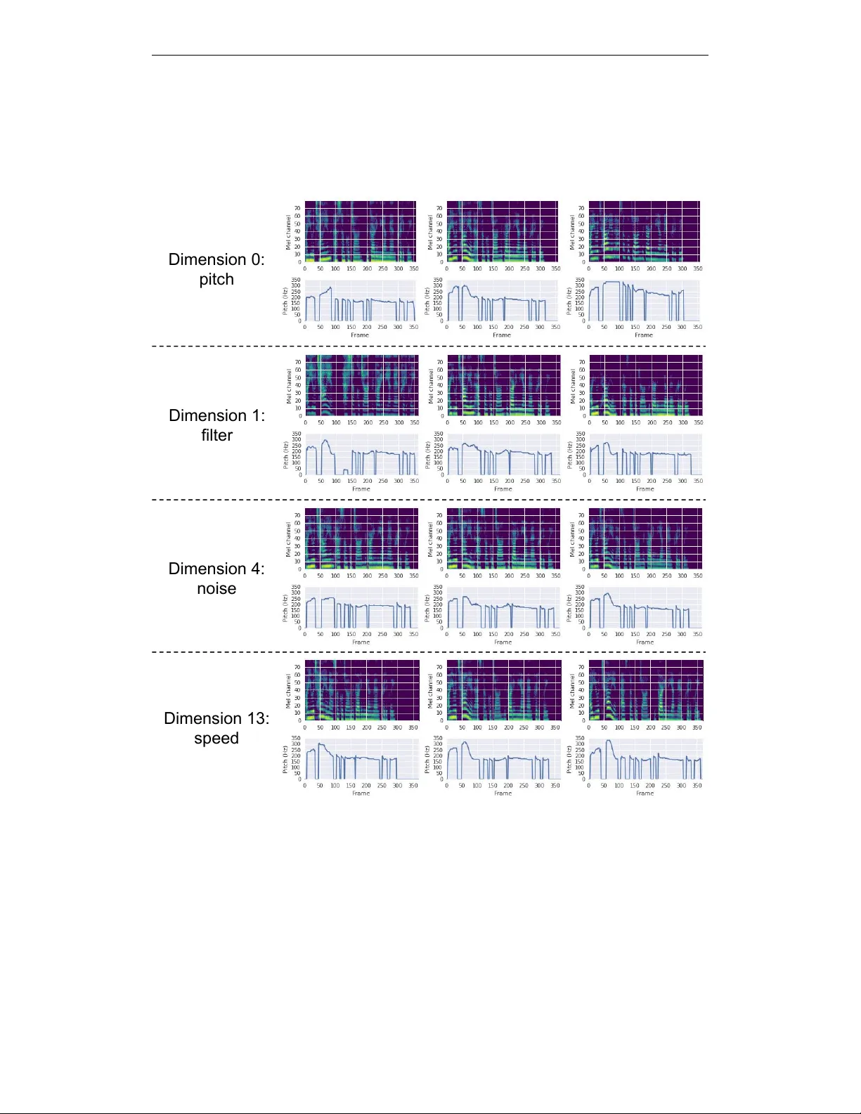
Published as a conference paper at ICLR 2019 H I E R A R C H I C A L G E N E R A T I V E M O D E L I N G F O R C O N T R O L L A B L E S P E E C H S Y N T H E S I S W ei-Ning Hsu 1 ∗ Y u Zhang 2 Ron J. W eiss 2 Heiga Zen 2 Y onghui W u 2 Y uxuan W ang 2 Y uan Cao 2 Y e Jia 2 Zhifeng Chen 2 Jonathan Shen 2 Patrick Nguyen 2 Ruoming Pang 2 1 Massachusetts Institute of T echnology 2 Google Inc. wnhsu@csail.mit.edu, { ngyuzh,ronw } @google.com A B S T R AC T This paper proposes a neural sequence-to-sequence text-to-speech (TTS) model which can control latent attributes in the generated speech that are rarely annotated in the training data, such as speaking style, accent, background noise, and record- ing conditions. The model is formulated as a conditional generati ve model based on the v ariational autoencoder (V AE) frame work, with two le vels of hierarchical latent v ariables. The ﬁrst le vel is a categorical v ariable, which represents attribute groups (e.g. clean/noisy) and provides interpretability . The second le vel, condi- tioned on the ﬁrst, is a multiv ariate Gaussian variable, which characterizes speciﬁc attribute conﬁgurations (e.g. noise le vel, speaking rate) and enables disentangled ﬁne-grained control ov er these attributes. This amounts to using a Gaussian mixture model (GMM) for the latent distrib ution. Extensiv e ev aluation demonstrates its ability to control the aforementioned attributes. In particular , we train a high-quality controllable TTS model on real found data, which is capable of inferring speaker and style attrib utes from a noisy utterance and use it to synthesize clean speech with controllable speaking style. 1 I N T RO D U C T I O N Recent development of neural sequence-to-sequence TTS models has shown promising results in generating high ﬁdelity speech without the need of handcrafted linguistic features (Sotelo et al., 2017; W ang et al., 2017; Arık et al., 2017; Shen et al., 2018). These models rely hea vily on a encoder- decoder neural network structure (Sutskev er et al., 2014; Bahdanau et al., 2015) that maps a text sequence to a sequence of speech frames. Extensions to these models have sho wn that attributes such as speaker identity can be controlled by conditioning the decoder on additional attribute labels (Arik et al., 2017; 2018; Jia et al., 2018). There are many speech attrib utes aside from speaker identity that are difﬁcult to annotate, such as speaking style, prosody , recording channel, and noise lev els. Skerry-Ryan et al. (2018); W ang et al. (2018) model such latent attributes through conditional auto-encoding, by extending the decoder inputs to include a vector inferred from the tar get speech which aims to capture the residual attributes that are not speciﬁed by other input streams, in addition to text and a speaker label. These models ha ve shown con vincing results in synthesizing speech that resembles the prosody or the noise conditions of the reference speech, which may not hav e the same text or speaker identity as the tar get speech. Nev ertheless, the presence of multiple latent attrib utes is common in crowdsourced data such as (Panayotov et al., 2015), in which prosody , speaker , and noise conditions all vary simultane- ously . Using such data, simply copying the latent attrib utes from a reference is insufﬁcient if one desires to synthesize speech that mimics the prosody of the reference, but is in the same noise condition as another . If the latent representation were disentangled , these generating factors could be controlled independently . Furthermore, it is can useful to construct a systematic method for synthesizing speech with random latent attributes, which would facilitate data augmentation (Tjandra et al., 2017; 2018; Hsu et al., 2017b; 2018; Hayashi et al., 2018) by generating di verse examples. These properties were not explicitly addressed in the pre vious studies, which model v ariation of a single latent attribute. ∗ W ork performed while interning at Google Brain. 1 Published as a conference paper at ICLR 2019 Motiv ated by the applications of sampling, inferring, and independently controlling individual attributes, we build off of Skerry-Ryan et al. (2018) and extend T acotron 2 (Shen et al., 2018) to model two separate latent spaces: one for labeled (i.e. related to speaker identity) and another for unlabeled attributes. Each latent v ariable is modeled in a variational autoencoding (Kingma & W elling, 2014) frame work using Gaussian mixture priors. The resulting latent spaces (1) learn disentangled attribute representations, where each dimension controls a different generating factor; (2) discover a set of interpretable clusters, each of which corresponds to a representative mode in the training data (e.g., one cluster for clean speech and another for noisy speech); and (3) provide a systematic sampling mechanism from the learned prior . The proposed model is e xtensively ev aluated on four datasets with subjective and objectiv e quantitative metrics, as well as comprehensive qualitati ve studies. Experiments conﬁrm that the proposed model is capable of controlling speaker , noise, and style independently , ev en when variation of all attrib utes is present but unannotated in the train set. Our main contributions are as follo ws: • W e propose a principled probabilistic hierarchical generativ e model, which impro ves (1) sam- pling stability and disentangled attribute control compared to e.g. the GST model of W ang et al. (2018), and (2) interpretability and quality compared to e.g. Akuzawa et al. (2018). • The model formulation explicitly factors the latent enc oding by using two mixture distribu- tions to separately model supervised speak er attributes and latent attributes in a disentangled fashion. This makes it straightforward to condition the model output on speak er and latent encodings inferred from different reference utterances. • T o the best of our kno wledge, this work is the ﬁrst to train a high-quality controllable te xt- to-speech system on real found data containing signiﬁcant variation in recording condition, speaker identity , as well as prosody and style. Previous results on similar data focused on speaker modeling (Ping et al., 2018; Nachmani et al., 2018; Arik et al., 2018; Jia et al., 2018), and did not explicitly address modeling of prosody and background noise. Lev eraging disentangled speaker and latent attrib ute encodings, the proposed model is capable of inferring the speaker attribute representation from a noisy utterance spoken by a previously unseen speaker , and using it to synthesize high-quality clean speech that approximates the voice of that speak er . 2 M O D E L T acotron-like TTS systems take a text sequence Y t and an optional observed categorical label (e.g. speaker identity) y o as input, and use an autoregressi ve decoder to predict a sequence of acoustic features X frame by frame. Training such a system to minimize a mean squared error reconstruction loss can be regarded as ﬁtting a probabilistic model p ( X | Y t , y o ) = Q n p ( x n | x 1 , x 2 , . . . , x n − 1 , Y t , y o ) that maximizes the lik elihood of generating the training data, where the conditional distrib ution of each frame x n is modeled as ﬁxed-v ariance isotropic Gaussian whose mean is predicted by the decoder at step n . Such a model ef fectively inte grates out other unlabeled latent attrib utes like prosody , and produces a conditional distribution with higher v ariance. As a result, the model would opaquely produce speech with unpredictable latent attrib utes. T o enable control of those attributes, we adopt a graphical model with hierarchical latent variables, which captures such attributes. Belo w we explain how the formulation leads to interpretability and disentanglement, supports sampling, and propose efﬁcient inference and training methods. 2 . 1 C O N D I T I O N A L G E N E R A T I V E M O D E L W I T H H I E R A R C H I C A L L A T E N T V A R I A B L E S T wo latent v ariables y l and z l are introduced in addition to the observed variables, X , Y t , and y o , as sho wn in the graphical model in the left of Figure 1. y l is a K -way cate gorical discrete variable, named latent attrib ute class , and z l is a D -dimensional continuous v ariable, named latent attribute r epr esentation . Throughout the paper , we use y ∗ and z ∗ to denote discrete and continuous variables, respectiv ely . T o generate speech X conditioned on the te xt Y t and observed attrib ute y o , y l is ﬁrst sampled from its prior , p ( y l ) , then a latent attribute representation z l is sampled from the conditional distribution p ( z l | y l ) . Finally , a sequence of speech frames is drawn from p ( X | Y t , y o , z l ) , parameterized by the synthesizer neural network. The joint probability can be written as: p ( X , y l , z l | Y t , y o ) = p ( X | Y t , y o , z l ) p ( z l | y l ) p ( y l ) . (1) 2 Published as a conference paper at ICLR 2019 text observed class latent class latent repr speech text observed class latent class latent repr observed repr speech Figure 1: Graphical model representation of the proposed models. Observed class often corresponds to the speaker label. The left illustrates equation 1, and the right illustrates the extension from Section 2.3. The grey and white nodes correspond to observed and latent v ariables. Speciﬁcally , it is assumed that p ( y l ) = K − 1 to be a non-informativ e prior to encourage every component to be used, and p ( z l | y l ) = N ( µ y l , diag ( σ y l )) to be diagonal-cov ariance Gaussian with learnable means and variances. As a result, the mar ginal prior of z l becomes a GMM with diagonal cov ariances and equal mixture weights. W e hope this GMM latent model can better capture the complexity of unseen attrib utes. Furthermore, in the presence of natural clusters of unseen attributes, the proposed model can achie ve interpretability by learning to assign instances from different clusters to different mixture components. The cov ariance matrix of each mixture component is constrained to be diagonal to encourage each dimension to capture a statistically uncorrelated factor . 2 . 2 V A R I A T I O N A L I N F E R E N C E A N D T R A I N I N G The conditional output distrib ution p ( X | Y t , y o , z l ) is parameterized with a neural network. Follow- ing the V AE frame work of Kingma & W elling (2014), a variational distrib ution q ( y l | X ) q ( z l | X ) is used to approximate the posterior p ( y l , z l | X , Y t , y o ) , which assumes that the posterior of unseen attributes is independent of the text and observed attributes. The approximated posterior for z l , q ( z l | X ) , is modeled as a Gaussian distrib ution with diagonal cov ariance matrix, whose mean and variance are parameterized by a neural network. For q ( y l | X ) , instead of introducing another neural network, we conﬁgure it to be an approximation of p ( y l | X ) that reuses q ( z l | X ) as follo ws: p ( y l | X ) = Z z l p ( y l | z l ) p ( z l | X ) d z l = E p ( z l | X ) [ p ( y l | z l )] ≈ E q ( z l | X ) [ p ( y l | z l )] := q ( y l | X ) (2) which enjoys the closed-form solution of Gaussian mixture posteriors, p ( y l | z l ) . Similar to V AE, the model is trained by maximizing its evidence lo wer bound (ELBO), as follows: L ( p, q ; X , Y t , y o ) = E q ( z l | X ) [log p ( X | Y t , y o , z l )] − E q ( y l | X ) [ D K L ( q ( z l | X ) || p ( z l | y l ))] − D K L ( q ( y l | X ) || p ( y l )) (3) where q ( z l | X ) is estimated via Monte Carlo sampling, and all components are differentiable thanks to reparameterization. Details can be found in Appendix A. 2 . 3 A C O N T I N U O U S A T T R I B U T E S PAC E F O R C A T E G O R I C A L O B S E RV E D L A B E L S Categorical observ ed labels, such as speaker identity , can often be seen as a categorization from a continuous attribute space, which for example could model a speak er’ s characteristic F 0 range and vocal tract shape. Gi ven an observed label, there may still be some variation of these attributes. W e are interested in learning this continuous attribute space for modeling within-class variation and inferring a representation from an instance of an unseen class for one-shot learning. T o achie ve this, a continuous latent variable, z o , named the observed attribute repr esentation , is introduced between the cate gorical observed label y o and speech X , as shown on the right of Figure 1. Each observed class (e.g. each speaker) forms a mixture component in this continuous space, whose conditional distribution is a diagonal-covariance Gaussian p ( z o | y o ) = N ( µ y o , diag ( σ y o )) . W ith this formulation, speech from an observed class y o is now generated by conditioning on Y t , z l , and a sample z o drawn from p ( z o | y o ) . As before, a variational distribution q ( z o | X ) , parameterized by a neural network, is used to approximate the true posterior , where the ELBO becomes: L o ( p, q ; X , Y t , y o ) = E q ( z o | X ) q ( z l | X ) [log p ( X | Y t , z o , z l )] − D K L ( q ( z o | X ) || p ( z o | y o )) − E q ( y l | X ) [ D K L ( q ( z l | X ) || p ( z l | y l ))] − D K L ( q ( y l | X ) || p ( y l )) . (4) 3 Published as a conference paper at ICLR 2019 observed encoder synthesizer latent encoder audio sequence text sequence latent attribute posterior observed attribute posterior text encodings decoder mel spectrogram Figure 2: Training conﬁguration of the GMV AE-T acotron model. Dashed lines denotes sampling. The model is comprised of three modules: a synthesizer , a latent encoder , and an observed encoder . T o encourage z o to disentangle observed attrib utes from latent attributes, the variances of p ( z o | y o ) are initialized to be smaller than those of p ( z l | y l ) . The intuition is that this space should capture v ariation of attributes that are highly correlated with the observed labels, so the conditional distribution of all dimensions should ha ve relativ ely small variance for each mixture component. Experimental results verify the ef fectiv eness, and similar design is used in Hsu et al. (2017a). In the extreme case where the variance is ﬁx ed and approaches zero, this formulation conv erges to using an lookup table. 2 . 4 N E U R A L N E T W O R K A R C H I T E C T U R E W e parameterize three distributions: p ( X | Y t , z o , z l ) (or p ( X | Y t , z o , z l ) ), q ( z o | X ) , and q ( z l | X ) with neural networks, referred to in Figure 2 as the synthesizer , observed encoder , and latent encoder , respectiv ely . The synthesizer is based on the T acotron 2 architecture (Shen et al., 2018), which consists of a te xt encoder and an autoregressi ve speech decoder . The former maps Y t to a sequence of text encodings Z t , and the latter predicts the mean of p ( x n | x 1 , . . . , x n − 1 , Z t , y o , z l ) at each step n . W e inject the latent variables z l and y o (or z o ) into the decoder by concatenating them to the decoder input at each step. T ext Y t and speech X are represented as a sequence of phonemes and a sequence of mel-scale ﬁlterbank coef ﬁcients, respectively . T o speed up inference, we use a W aveRNN-based neural vocoder (Kalchbrenner et al., 2018) instead of W a veNet (van den Oord et al., 2016), to in vert the predicted mel-spectrogram to a time-domain wa veform. The two posteriors, q ( z l | X ) and q ( z o | X ) , are both parameterized by a recurrent encoder that maps a v ariable-length mel-spectrogram to two ﬁxed-dimensional v ectors, corresponding to the posterior mean and log variance, respecti vely . Full architecture details can be found in Appendix B. 3 R E L A T E D W O R K The proposed GMV AE-T acotron model is most related to Skerry-Ryan et al. (2018), W ang et al. (2018), Henter et al. (2018), which introduce a reference embedding to model prosody or noise. The ﬁrst uses an autoencoder to extract a prosody embedding from a reference speech spectrogram. The second Global Style T oken (GST) model constrains a reference embedding to be a weighted combination of a ﬁxed set of learned vectors, while the third further restricts the weights to be one-hot, and is b uilt on a con ventional parametric speech synthesizer (Zen et al., 2009). The main focus of these approaches was style transfer from a reference audio example. They provide neither a systematic sampling mechanism nor disentangled representations as we show in Section 4.3.1. Similar to these approaches, Akuzaw a et al. (2018) extend V oiceLoop (T aigman et al., 2018) with a latent reference embedding generated by a V AE, using a centered ﬁx ed-variance isotropic Gaussian prior for the latent attrib utes. This pro vides a principled mechanism for sampling from the latent distribution, but does not provide interpretability . In contrast, GMV AE-T acotron models latent attributes using a mixture distrib ution, which allows automatic disco very of latent attribute clusters. This structure makes it easier to interpret the underlying latent space. Speciﬁcally , we show in Section 4.1 that the mixture parameters can be analyzed to understand what each component corresponds to, similar to GST . In addition, the most distincti ve dimensions of the latent space can be identiﬁed using an inter-/intra-component v ariance ratio, which e.g. can identify the dimension controlling the background noise lev el as shown in Section 4.2.2. Finally , the extension described in Section 2.3 adds a second mixture distribution to additionally models speaker attrib utes. This formulation learns disentangled speaker and latent attribute represen- 4 Published as a conference paper at ICLR 2019 tations, which can be used to approximate the voice of speakers pre viously unseen during training. This speaker model is related to Arik et al. (2018), which controls the output speaker identity using speaker embeddings, and trains a separate regression model to predict them from the audio. This can be regarded as a special case of the proposed model where the variance of z o is set to be almost zero, such that a speaker always generates a ﬁxed representation; meanwhile, the posterior model q ( z o | X ) corresponds to their embedding predictor , because it now aims to predict a ﬁxed embedding for each speaker . Using a mixture distribution for latent variables in a V AE was e xplored in Dilokthanakul et al. (2016); Nalisnick et al. (2016), and Jiang et al. (2017) for unconditional image generation and text topic modeling. These models correspond to the sub-graph y l → z l → X in Figure 1. The proposed model provides extra ﬂe xibility to model both latent and observed attrib utes in a conditional generation scenario. Hsu et al. (2017a) similarly learned disentangled representations at the v ariable lev el (i.e. disentangling z l and z o ) by deﬁning different priors for different latent v ariables. Higgins et al. (2017) also used a prior with diagonal covariance matrix to disentangle different embedding dimensions. Our model provides additional ﬂexibility by learning a dif ferent variance in each mixture component. 4 E X P E R I M E N T S The proposed GMV AE-T acotron was e valuated on four datasets, spanning a wide degree of variations in speaker , recording channel conditions, background noise, prosody , and speaking styles. For all experiments, y o was an observed cate gorical variable whose cardinality is the number of speakers in the training set if used, y l was conﬁgured to be a 10-way cate gorical variable ( K = 10 ), and z l and z o (if used) were conﬁgured to be 16-dimensional variables ( D = 16 ). T acotron 2 (Shen et al., 2018) with a speaker embedding table w as used as the baseline for all experiments. F or all other variants (e.g., GST), the reference encoder follo ws W ang et al. (2018). Each model w as trained for at least 200k steps to maximize the ELBO in equation 3 or equation 4 using the Adam optimizer . A list of detailed hyperparameter settings can be found in Appendix C. Quantitati ve subjectiv e ev aluations relied on crowd-sourced mean opinion scores (MOS) rating the naturalness of the synthesized speech by nati ve speakers using headphones, with scores ranging from 1 to 5 in increments of 0.5. For single speaker datasets each sample was rated by 6 raters, while for other datasets each sample was rated by a single rater . W e strongly encourage readers to listen to the samples on the demo page. 1 4 . 1 M U LT I - S P E A K E R E N G L I S H C O R P U S T o evaluate the ability of GMV AE-T acotron to model speaker variation and discover meaningful speaker clusters, we used a proprietary dataset of 385 hours of high-quality English speech from 84 professional voice talents with accents from the United States (US), Great Britain (GB), Australia (A U), and Singapore (SG). Speaker labels were not seen during training ( y o and z o were unused), and were only used for ev aluation. Figure 3: Assignment distribution ov er y l for each gender (upper) and for each accent (lower). T o probe the interpretability of the model, we computed the distribution of mixture components y l for utterances of a par - ticular accent or gender . Speciﬁcally , we collected at most 100 utterances from each of the 44 speakers with at least 20 test utter- ances (2,332 in total), and assigned each utterance to the compo- nent with the highest posterior probability: arg max y l q ( y l | X ) . Figure 3 plots the assignment distributions for each gender and accent in this set. Most components were only used to model speakers from one gender . Each component which modeled both genders (0, 2, and 9) only represented a subset of accents (US, US, and A U/GB, respectiv ely). W e also found that the sev eral components which modeled US female speakers (3, 5, and 6) actually modeled groups of speakers with distinct char - acteristics, e.g. dif ferent F 0 ranges as sho wn in Appendix E. T o quantify the association between speak er and mixture compo- nents, we computed the assignment consistency w .r .t. speaker: 1 https://google.github.io/tacotron/publications/gmvae_controllable_tts 5 Published as a conference paper at ICLR 2019 Figure 4: Left: Euclidean distance between the means of each mixture component pair . Right: De- coding the same text conditioned on the mean of a noisy (center) and a clean component (right). 1 M P N i =1 P N i j =1 1 y ij = ˆ y i where M is the number of utterances, y ij is the component assignment of utterance j from speaker i , and ˆ y i is the mode of { y ij } N i j =1 . The resulting consistency was 92 . 9% , suggesting that the components group utterances by speaker and group speakers by gender or accent. W e also explored what each dimension of z l controlled by decoding with different values of the target dimension, keeping all other factors ﬁxed. W e discovered that there were indi vidual dimensions which controlled F 0 , speaking rate, accent, length of starting silence, etc., demonstrating the disentangled nature of the learned latent attribute representation. Appendix E contains visualization of attribute control and additional quantitativ e ev aluation of using z l for gender/accent/speaker classiﬁcation. 4 . 2 N O I S Y M U LTI - S P E A K E R E N G L I S H C O R P U S High quality data can be both expensiv e and time consuming to record. V ast amounts of rich real-life expressi ve speech are often noisy and difﬁcult to label. In this section we demonstrate that our model can synthesize clean speech directly from noisy data by disentangling the background noise lev el from other attributes, allo wing it to be controlled independently . As a ﬁrst experiment, we artiﬁcially generated training sets using a room simulator (Kim et al., 2017) to add background noise and rev erberation to clean speech from the multi-speaker English corpus used in the previous section. W e used music and ambient noise sampled from Y ouT ube and recordings of “daily life” en vironments as noise signals, mix ed at signal-to-noise ratios (SNRs) ranging from 5–25dB. The rev erberation time vari ed between 100 and 900ms. Noise was added to a random selection of 50% of utterances by each speaker , holding out two speakers (one male and one female) for whom noise was added to all of their utterances. This construction was used to e valuate the ability of the model to synthesize clean speech for speakers whose training utterances were all corrupted by noise. In this experiment, we provided speak er labels y o as input to the decoder , and only expect the latent attribute representations z l to capture the acoustic condition of each utterance. 4 . 2 . 1 I D E N T I F Y I N G M I X T U R E C O M P O N E N T S T H A T G E N E R A T E C L E A N / N O I S Y S P E E C H Unlike clustering speak ers, we expected that latent attrib utes would naturally di vide into two cate- gories: clean and noisy . T o verify this hypothesis, we plotted the Euclidean distance between means of each pair of components on the left of Figure 4, which clearly form two distinct clusters. The right two plots in Figure 4 show the mel-spectrograms of two synthesized utterances of the same text and speaker , conditioned on the means of two different components, one from each group. It clearly presents the samples (in fact, all the samples) dra wn from components in group one were noisy , while the samples drawn from the other components were clean. See Appendix F for more examples. 4 . 2 . 2 C O N T RO L O F T H E BA C K G R O U N D N O I S E L E V E L W e next explored if the le vel of noise was dominated by a single latent dimension, and whether we could determine such a dimension automatically . For this purpose, we adopted a per-dimension LDA, which computed a between and within-mixture scattering ratio: r d = P K y l =1 p ( y l )( µ y l ,d − ¯ µ l,d ) 2 / P K y l =1 p ( y l ) σ 2 y l ,d , where µ y l ,d and σ y l ,d are the d -th dimension mean and v ariance of mixture component y l , and ¯ µ l,d is the d -th dimension mean of the marginal dis- tribution p ( z l ) = P K y l =1 p ( y l ) p ( z l | y l ) . This is a scale-inv ariant metric of the degree of separation between components in each latent dimension. W e discov ered that the most discriminative dimension had a scattering ratio r 13 = 21 . 5 , far larger than the second largest r 11 = 0 . 6 . Drawing samples and trav ersing values along the target dimension 6 Published as a conference paper at ICLR 2019 ¯ µ l , d − 2 ¯ σ l , d ¯ µ l , d − ¯ σ l , d ¯ µ l , d ¯ µ l , d + ¯ σ l , d ¯ µ l , d + 2 ¯ σ l , d Target dimension value 0 5 10 15 WADA SNR (dB) Clean component (5) ¯ µ l , d − 2 ¯ σ l , d ¯ µ l , d − ¯ σ l , d ¯ µ l , d ¯ µ l , d + ¯ σ l , d ¯ µ l , d + 2 ¯ σ l , d Target dimension value Noisy component (0) dim 0 dim 1 dim 2 dim 3 dim 4 dim 5 dim 6 dim 7 dim 8 dim 9 dim 10 dim 11 dim 12 dim 13 dim 14 dim 15 Figure 5: SNR as a function of the value in each latent dimen- sion, comparing clean (left) and noisy (right) components. T able 1: MOS and SNR comparison among clean original audio, baseline, GST , V AE, and GMV AE models. Model MOS SNR Original 4.48 ± 0.04 17.71 Baseline 2.87 ± 0.25 11.56 GST 3.32 ± 0.13 14.43 V AE 3.55 ± 0.17 12.91 GMV AE 4.25 ± 0.13 17.20 while keeping others ﬁxed demonstrates that dimension’ s effect on the output. T o determine the effecti ve range of the target dimension, we approximate the multimodal distribution as a Gaussian and e valuate v alues spanning four standard deviations ¯ σ l,d around the mean. T o quantify the ef fect on noise lev el, we estimate the SNR without a reference clean signal following Kim & Stern (2008). Figure 5 plots the average estimated SNR o ver 200 utterances from two speakers as a function of the v alue in each latent dimension, where values for other dimensions are the mean of a clean component (left) or that of a noisy component (right). The results sho w that the noise le vel was clearly controlled by manipulating the 13 th dimension, and remains nearly constant as the other dimensions vary , verifying that control has been isolated to the identiﬁed dimension. The small degree of v ariation, e.g. in dimensions 2 and 4, occurs because some of those dimensions control attributes which directly affect the synthesized noise, such as type of noise (musical/white noise) and initial background noise offset, and therefore also af fect the estimated SNR. Appendix F .2 contains an additional spectrogram demonstration of noise lev el control by manipulating the identiﬁed dimension. 4 . 2 . 3 S Y N T H E S I Z I N G C L E A N S P E E C H F O R N O I S Y S P E A K E R S In this section, we ev aluated synthesis quality for the two held out noisy speakers. Ev aluation metrics included subjective naturalness MOS ratings and an objecti ve SNR metric. T able 1 compares the proposed model with a baseline, a 16-token GST , and a V AE v ariant which replaces the GMM prior with an isotropic Gaussian. T o encourage synthesis of clean audio under each model we manually selected the cleanest token (weight = 0.15) for GST , used the Gaussian prior mean (i.e. a zero vector) for V AE, and the mean of a clean component for GMV AE. For the V AE model, the mean captured the average condition, which still exhibited a moderate le vel of noise, resulting in a lo wer SNR and MOS. The generated speech from the GST was cleaner, ho wev er raters sometimes found its prosody to be unnatural. Note that it is possible that another token would obtain a different trade-of f between prosody and SNR, and using multiple tokens could improve both. Finally , the proposed model synthesized both natural and high-quality speech, with the highest MOS and SNR. 4 . 3 S I N G L E - S P E A K E R AU D I O B O O K C O R P U S Prosody and speaking style is another important factor for human speech other than speaker and noise. Control of these aspects of the synthesize speech is essential to building an expressi ve TTS system. In this section, we ev aluated the ability of the proposed model to sample and control speaking styles. A single speaker US English audiobook dataset of 147 hours, recorded by professional speaker , Catherine Byers, from the 2013 Blizzard Challenge (King & Karaiskos, 2013) is used for training. The data incorporated a wide range of prosody v ariation. W e used an ev aluation set of 150 audiobook sentences, including many long phrases. T able 2 shows the naturalness MOS between baseline and proposed model conditioning on the same z l , set to the mean of a selected y l , for all utterances. The results sho w that the prior already captured a common prosody , which could be used to synthesize more naturally sounding speech with a lower v ariance compared to the baseline. 7 Published as a conference paper at ICLR 2019 T able 2: MOS comparison of the original audio, base- line and GMV AE. Model MOS Original 4.67 ± 0.04 Baseline 4.29 ± 0.11 Proposed 4.67 ± 0.07 Figure 6: Mel-spectrograms of three samples with the same text, “W e must burn the house down! said the Rabbit’ s voice. ” dra wn from the proposed model, showing v ariation in speed, F 0 , and pause duration. (a) (b) Figure 7: (a) Mel-spectrograms of two unnatural GST samples when setting the weight for one token -0.1: ﬁrst with tremolo at the end, and second with abnormally long duration for the ﬁrst syllable. (b) F 0 tracks and spectrograms from GMV AE-T acotron using different v alues for the “speed” dimension. 4 . 3 . 1 S T Y L E S A M P L I N G A N D D I S E N TA N G L E D C O N T R O L Compared to GST , one primary advantage of the proposed model is that it supports random sampling of natural speech from the prior . Figure 6 illustrates such samples, where the same text is synthesized with wide variation in speaking rate, rhythm, and F 0 . In contrast, the GST model does not deﬁne a prior for normalized token weights, requiring weights to be chosen heuristically or by ﬁtting a distribution after training. Empirically we found that the GST weight simplex was not fully exploited during training and that careful tuning was required to ﬁnd a stable sampling region. An additional adv antage of GMV AE-T acotron is that it learns a representation which disentangles these attributes, enabling them to be controlled independently . Speciﬁcally , latent dimensions in the proposed model are conditionally independent, while token weights of GST are in fact correlated. Figure 7(b) contains an example of the proposed model tra versing the “speed” dimension with three values: ¯ µ l,d − 2 ¯ σ l,d , ¯ µ l,d , ¯ µ l,d + 2 ¯ σ l,d , plotted accordingly from left to right, where ¯ µ l,d and ¯ σ l,d are the marginal distribution mean and standard de viation, respecti vely , of that dimension. Their F 0 tracks, obtained using the YIN (De Che veign ´ e & Kaw ahara, 2002) F 0 tracker , are shown on the left. From these we can observe that the shape of the F 0 contours did not change much. They were simply stretched horizontally , indicating that only the speed was manipulated. In contrast, the style control of GST is more entangled, as shown in W ang et al. (2018, Figure 3(a)), where the F 0 also changed while controlling speed. Appendix G contains a quantitativ e analysis of disentangled latent attribute control, and additional ev aluation of style transfer, demonstrating the ability of the proposed the model to synthesize speech that resembles the prosody of a reference utterance. 4 . 4 C R O W D - S O U R C E D AU D I O B O O K C O R P U S W e used an audiobook dataset 2 deriv ed from the same subset of LibriV ox audiobooks used for the LibriSpeech corpus (Panayoto v et al., 2015), but sampled at 24kHz and se gmented dif ferently , making it appropriate for TTS instead of speech recognition. The corpus contains recordings from thousands of speakers, with wide variation in recording conditions and speaking style. Speaker identity is often highly correlated with the recording channel and background noise level, since man y speakers tended to use the same microphone in a consistent recording environment. The ability to disentangle and control these attributes independently is essential to synthesizing high-quality speech for all speakers. 2 This dataset will be open-sourced soon. 8 Published as a conference paper at ICLR 2019 T able 3: SNR of original audio, baseline, and the proposed models with different conditioned z l , on different speak ers. Set Original Baseline Proposed mean latent latent-dn SC 18.61 14.33 15.90 16.28 17.94 SN 11.80 9.69 15.82 6.78 18.94 UC 20.39 N/A 15.70 16.40 18.83 UN 10.92 N/A 15.27 4.81 16.89 T able 4: Subjecti ve preference (%) between baseline and proposed model with denoised z l on the set of “seen noisy” (SN) speakers. Baseline Neutral Proposed 4.0 10.5 85.5 W e augmented the model with the z o layer described in Section 2.3 to learn a continuous speaker representation and an inference model for it. The train-clean- { 100,360 } partitions were used for training, which spans 1,172 unique speak ers and, despite the name, includes man y noisy recordings. As in previous e xperiments, by trav ersing each dimension of z l we found that dif ferent latent dimensions independently control dif ferent attributes of the generated speech. Moreov er , this representation was disentangled from speaker identity , i.e. modifying z l did not affect the generated speaker identity if z o was ﬁxed. In addition, we discov ered that the mean of one mixture component corresponded to a narrati ve speaking style in a clean recording condition. Demonstrations of latent attribute control are sho wn in Appendix H and the demo page. 4 . 4 . 1 C L E A N S Y N T H E S I S F O R S P E A K E R S W I T H N O I S Y T R A I N I N G DAT A W e demonstrate the ability of GMV AE-T acotron to consistently generate high-quality speech by conditioning on a value of z l associated with clean output. W e considered two approaches: (1) using the mean of the identiﬁed clean component, which can be seen as a preset conﬁguration with a ﬁxed channel and style; (2) inferring a latent attribute representation z l from reference speech and denoising it by modifying dimensions 3 associated with the noise lev el to predetermined values. W e e valuated a set of eight “seen clean” (SC) speakers and a set of nine “seen noisy” (SN) speak ers from the training set, a set of ten “unseen noisy” (UN) speakers from a held-out set with no ov erlapping speakers, and the set of ten unseen speakers used in Jia et al. (2018), denoted as “unseen clean” (UC). For consistenc y , we always used an inferred z o from an utterance from the target speaker , regardless of whether that speaker was seen or unseen. As a baseline we used a T acotron model conditioned on a 128-dimensional speaker embedding learned for each speaker seen during training. T able 3 sho ws the SNR of the original audio, audio synthesized by the baseline, and by the GMV AE- T acotron using the tw o proposed approaches, denoted as mean and latent-dn , respectively , on all speaker sets whene ver possible. In addition, to see the ef fectiv eness of the denoising operation, the table also includes the results of using inferred z l directly , denoted as latent . The results sho w that the inferred z l followed the same SNR trend as the original audio, indicating that z l captured the variation in acoustic condition. The high SNR values of mean and latent-dn v eriﬁes the effecti veness of using a preset and denoising arbitrary inferred latent features, both of which outperformed the baseline by a large mar gin, and produced better quality than the original noisy audio. T able 4 compares the proposed model using denoised z l to the baseline in a subjectiv e side-by- side preference test. T able 5 further compares subjective naturalness MOS of the proposed model using the mean of the clean component to the baseline on the two seen speaker sets, and to the d -vector model (Jia et al., 2018) on the two unseen speaker sets. Speciﬁcally , we consider another stronger baseline model to compare on the SN set, which is trained on denoised data using spectral subtraction (Boll, 1979), denoted as “ + denoise . ” Both results indicate that raters preferred the proposed model to the baselines. Moreover , the MOS ev aluation sho ws that the proposed model deliv ered similar lev el of naturalness under all conditions, seen or unseen, clean or noisy . 3 W e found two rele vant dimensions, controlling 1) lo w frequency , narrowband, and 2) wideband noise le vels. 9 Published as a conference paper at ICLR 2019 T able 5: Naturalness MOS of original audio, baseline, and proposed model with the clean component mean. Set Model MOS SC Original 4.60 ± 0.07 Baseline 4.17 ± 0.07 Proposed 4.18 ± 0.06 SN Original 4.45 ± 0.08 Baseline 3.64 ± 0.10 + denoise 3.84 ± 0.10 Proposed 4.09 ± 0.08 UC Original 4.54 ± 0.08 d -vector 4.10 ± 0.06 Proposed 4.26 ± 0.05 UN Original 4.34 ± 0.07 d -vector 3.76 ± 0.12 Proposed 4.20 ± 0.08 T able 6: Speaker similarity MOS. Set Model MOS SC Baseline 3.54 ± 0.09 Proposed 3.60 ± 0.09 SN Original 3.30 ± 0.27 (different channels) Baseline 3.83 ± 0.08 Baseline + denoise 3.23 ± 0.20 Proposed 3.11 ± 0.08 UC d -vector 2.23 ± 0.08 d -vector (lar ge) 3.03 ± 0.09 Proposed 2.79 ± 0.08 4 . 4 . 2 S P E A K E R S I M I L A R I T Y W e ev aluate whether the synthesized speech resembles the identity of the reference speaker , by pairing each synthesized utterance with the reference utterance for subjecti ve MOS e valuation of speaker similarity , follo wing Jia et al. (2018). T able 6 compares the proposed model using denoised latent attribute representations to baseline systems on the two seen speak er sets, and to d -vector systems on the unseen clean speaker set. The d -vector systems used a separately trained speaker encoder model to e xtract speaker representations for TTS conditioning as in Jia et al. (2018). W e considered two speaker encoder models, one trained on the same train-clean partition as the proposed model, and another trained on a larger scale dataset containing 18K speakers. W e denote these two systems as d -vector and d -vector (lar ge) . On the seen clean speaker set, the proposed model achieved similar speak er similarity scores to the baseline. Howe ver , on the seen noisy speaker set, both the proposed model and the baseline trained on denoised speech performed signiﬁcantly worse than the baseline. W e hypothesize that similarity of the acoustic conditions between the paired utterances biased the speaker similarity ratings. T o conﬁrm this hypothesis, we additionally e valuated speaker similarity of the ground truth utterances from a speaker whose recordings contained signiﬁcant variation in acoustic conditions. As shown in T able 6, these ground truth utterances were also rated with a signiﬁcantly lower MOS than the baseline, but were close to the proposed model and the denoised baseline. This result implies that this subjectiv e speaker similarity test may not be reliable in the presence of noise and channel variation, requiring additional work to design a speaker similarity test that is unbiased to such nuisance factors. Finally , on the unseen clean speaker set, the proposed model achieved signiﬁcantly better speaker similarity scores than the d -vector system whose speaker representation e xtractor was trained on the same set as the proposed model, but worse than the d -vector (large) system which was trained on ov er 15 times more speakers. Ho wev er, we emphasize that: (1) this is not a fair comparison as the two models are trained on datasets of dif ferent sizes, and (2) our proposed model is complementary to d -vector systems. Incorporating the high quality speaker transfer from the d -vector model with the strong controllability of the GMV AE is a promising direction for future work. 5 C O N C L U S I O N W e describe GMV AE-T acotron, a TTS model which learns an interpretable and disentangled latent representation to enable ﬁne-grained control of latent attrib utes and provides a systematic sampling scheme for them. If speaker labels are a vailable, we demonstrate an e xtension of the model that learns a continuous space that captures speaker attributes, along with an inference model which enables one-shot learning of speaker attrib utes from unseen reference utterances. 10 Published as a conference paper at ICLR 2019 The proposed model was extensiv ely ev aluated on tasks spanning a wide range of signal variation. W e demonstrated that it can independently control many latent attrib utes, and is able to cluster them without supervision. In particular , we veriﬁed using both subjectiv e and objectiv e tests that the model could synthesize high-quality clean speech for a target speaker even if the quality of data for that speaker does not meet high standard. These e xperimental results demonstrated the effecti veness of the model for training high-quality controllable TTS systems on lar ge scale training data with rich styles by learning to factorize and independently control latent attributes underlying the speech signal. A C K N O W L E D G M E N T S The authors thank Daisy Stanton, Rif A. Saurous, W illiam Chan, RJ Skerry-Ryan, Eric Battenber g, and the Google Brain, Perception and TTS teams for their helpful feedback and discussions. R E F E R E N C E S Kei Akuza wa, Y usuke Iwasa wa, and Y utaka Matsuo. Expressiv e speech synthesis via modeling expressions with v ariational autoencoder . In Interspeec h , pp. 3067–3071, 2018. W illiam Apple, L ynn A Streeter , and Robert M Krauss. Effects of pitch and speech rate on personal attributions. Journal of P ersonality and Social Psychology , 1979. Sercan Arık, Mike Chrzanowski, Adam Coates, Gregory Diamos, Andrew Gibiansky , Y ongguo Kang, Xian Li, John Miller , Andrew Ng, Jonathan Raiman, et al. Deep Voice: Real-time neural text-to-speech. In International Conference on Mac hine Learning (ICML) , pp. 195–204, 2017. Sercan Arik, Gregory Diamos, Andrew Gibiansk y , John Miller, Kainan Peng, W ei Ping, Jonathan Raiman, and Y anqi Zhou. Deep Voice 2: Multi-speaker neural te xt-to-speech. In Advances in Neural Information Pr ocessing Systems (NIPS) , 2017. Sercan Arik, Jitong Chen, Kainan Peng, W ei Ping, and Y anqi Zhou. Neural voice cloning with a fe w samples. arXiv pr eprint arXiv:1802.06006 , 2018. Dzmitry Bahdanau, Kyunghyun Cho, and Y oshua Bengio. Neural machine translation by jointly learning to align and translate. In International Confer ence on Learning Representations (ICLR) , 2015. John W Black. Relationships among fundamental frequency , v ocal sound pressure, and rate of speaking. Languag e and Speech , 1961. Stev en Boll. Suppression of acoustic noise in speech using spectral subtraction. IEEE T ransactions on Acoustics, Speech, and Signal Pr ocessing , 27(2):113–120, 1979. Samuel R Bo wman, Luke V ilnis, Oriol V inyals, Andrew Dai, Rafal Jozefowicz, and Samy Bengio. Generating sentences from a continuous space. In SIGNLL Conference on Computational Natural Language Learning (CoNLL) , 2016. Jan K Chorowski, Dzmitry Bahdanau, Dmitriy Serdyuk, Kyunghyun Cho, and Y oshua Bengio. Attention-based models for speech recognition. In Advances in Neural Information Pr ocessing Systems (NIPS) , 2015. Alain De Chev eign ´ e and Hideki Kawahara. YIN, a fundamental frequency estimator for speech and music. The J ournal of the Acoustical Society of America , 111(4):1917–1930, 2002. Nat Dilokthanakul, Pedro AM Mediano, Marta Garnelo, Matthew CH Lee, Hugh Salimbeni, Kai Arulkumaran, and Murray Shanahan. Deep unsupervised clustering with Gaussian mixture variational autoencoders. arXiv pr eprint arXiv:1611.02648 , 2016. Xavier Glorot and Y oshua Bengio. Understanding the dif ﬁculty of training deep feedforward neural networks. In Pr oceedings of the thirteenth international confer ence on artiﬁcial intelligence and statistics , pp. 249–256, 2010. 11 Published as a conference paper at ICLR 2019 T omoki Hayashi, Shinji W atanabe, Y u Zhang, T omoki T oda, T akaaki Hori, Ramon Astudillo, and Kazuya T akeda. Back-translation-style data augmentation for end-to-end ASR. arXiv pr eprint arXiv:1807.10893 , 2018. Gustav Eje Henter, Jaime Lorenzo-Trueba, Xin W ang, and Junichi Y amagishi. Deep encoder- decoder models for unsupervised learning of controllable speech synthesis. arXiv pr eprint arXiv:1807.11470 , 2018. Irina Higgins, Loic Matthey , Arka Pal, Christopher Burgess, Xavier Glorot, Matthew Botvinick, Shakir Mohamed, and Alexander Lerchner . beta-V AE: Learning basic visual concepts with a constrained variational frame work. In International Confer ence on Learning Representations (ICLR) , 2017. W ei-Ning Hsu, Y u Zhang, and James Glass. Unsupervised learning of disentangled and interpretable representations from sequential data. In Advances in Neural Information Pr ocessing Systems (NIPS) , 2017a. W ei-Ning Hsu, Y u Zhang, and James Glass. Unsupervised domain adaptation for rob ust speech recognition via variational autoencoder-based data augmentation. In Automatic Speech Recognition and Understanding W orkshop (ASR U) , pp. 16–23, 2017b. W ei-Ning Hsu, Hao T ang, and James Glass. Unsupervised adaptation with interpretable disentangled representations for distant con versational speech recognition. In Interspeech , pp. 1576–1580, 2018. Y e Jia, Y u Zhang, Ron J W eiss, Quan W ang, Jonathan Shen, Fei Ren, Zhifeng Chen, Patrick Nguyen, Ruoming Pang, Ignacio Lopez Moreno, et al. T ransfer learning from speaker veriﬁcation to multispeaker text-to-speech synthesis. arXiv pr eprint arXiv:1806.04558 , 2018. Zhuxi Jiang, Y in Zheng, Huachun T an, Bangsheng T ang, and Hanning Zhou. V ariational deep em- bedding: an unsupervised and generative approach to clustering. In International Joint Confer ence on Artiﬁcial Intelligence (IJCAI) , 2017. Nal Kalchbrenner , Erich Elsen, Karen Simonyan, Seb Noury , Norman Casagrande, Edward Lockhart, Florian Stimberg, A ¨ aron van den Oord, Sander Dieleman, and K oray Kavukcuoglu. Efﬁcient neural audio synthesis. In International Confer ence on Machine Learning (ICML) , 2018. Chanwoo Kim and Richard M Stern. Robust signal-to-noise ratio estimation based on waveform amplitude distribution analysis. In Interspeech , pp. 2598–2601, 2008. Chanwoo Kim, Anan ya Misra, Kean Chin, Thad Hughes, Arun Narayanan, T ara Sainath, and Michiel Bacchiani. Generation of large-scale simulated utterances in virtual rooms to train deep-neural networks for far -ﬁeld speech recognition in Google Home. In Interspeec h , pp. 379–383, 2017. Y oon Kim, Sam W iseman, Andrew C Miller , David Sontag, and Alexander M Rush. Semi-amortized variational autoencoders. 2018. Simon King and V asilis Karaiskos. The Blizzard Challenge 2013. In Blizzar d Challenge W orkshop , 2013. Diederik P Kingma and Jimmy Ba. Adam: A method for stochastic optimization. In International Confer ence on Learning Repr esentations (ICLR) , 2015. Diederik P Kingma and Max W elling. Auto-encoding v ariational Bayes. In International Conference on Learning Repr esentations (ICLR) , 2014. LibriV ox. https://librivox.org , 2005. Eliya Nachmani, Adam Polyak, Y ani v T aigman, and Lior W olf. Fitting new speakers based on a short untranscribed sample. arXiv pr eprint arXiv:1802.06984 , 2018. Eric Nalisnick, Lars Hertel, and Padhraic Smyth. Approximate inference for deep latent Gaussian mixtures. In NIPS W orkshop on Bayesian Deep Learning , 2016. 12 Published as a conference paper at ICLR 2019 V assil Panayoto v , Guoguo Chen, Daniel Pove y , and Sanjeev Khudanpur . LibriSpeech: An ASR corpus based on public domain audio books. In International Conference on Acoustics, Speec h and Signal Pr ocessing (ICASSP) , pp. 5206–5210, 2015. W ei Ping, Kainan Peng, Andre w Gibiansky , Sercan O Arik, Ajay Kannan, Sharan Narang, Jonathan Raiman, and John Miller . Deep Voice 3: 2000-speaker neural text-to-speech. In International Confer ence on Learning Repr esentations (ICLR) , 2018. Jonathan Shen, Ruoming P ang, Ron J W eiss, Mike Schuster, Navdeep Jaitly , Zongheng Y ang, Zhifeng Chen, Y u Zhang, Y uxuan W ang, RJ Skerry-Ryan, et al. Natural TTS synthesis by conditioning wa venet on mel spectrogram predictions. In International Confer ence on Acoustics, Speech and Signal Pr ocessing (ICASSP) , pp. 4779–4783, 2018. RJ Skerry-Ryan, Eric Battenber g, Y ing Xiao, Y uxuan W ang, Daisy Stanton, Joel Shor , Ron J W eiss, Rob Clark, and Rif A Saurous. T owards end-to-end prosody transfer for expressiv e speech synthesis with Tacotron. In International Confer ence on Machine Learning (ICML) , 2018. J. Sotelo, S. Mehri, K. Kumar , J. Santos, K. Kastner, A. Courville, and Y . Bengio. Char2Wav: End-to-End speech synthesis. In International Conference on Learning Repr esentations (ICLR) , 2017. Ilya Sutske ver , Oriol V inyals, and Quoc V Le. Sequence to sequence learning with neural networks. In Advances in Neural Information Pr ocessing Systems (NIPS) , 2014. Y aniv T aigman, Lior W olf, Adam Polyak, and Eliya Nachmani. V oiceLoop: Voice ﬁtting and synthesis via a phonological loop. In International Confer ence on Learning Repr esentations (ICLR) , 2018. Andros Tjandra, Sakriani Sakti, and Satoshi Nakamura. Listening while speaking: Speech chain by deep learning. In Automatic Speech Recognition and Understanding W orkshop (ASRU) , pp. 301–308, 2017. Andros Tjandra, Sakriani Sakti, and Satoshi Nakamura. Machine speech chain with one-shot speaker adaptation. In Interspeec h , pp. 887–891, 2018. A ¨ aron v an den Oord, Sander Dieleman, Heiga Zen, Karen Simonyan, Oriol V inyals, Alex Gra ves, Nal Kalchbrenner , Andrew Senior , and Koray Ka vukcuoglu. W a veNet: A generativ e model for raw audio. arXiv preprint , 2016. Ashish V aswani, Noam Shazeer , Niki Parmar , Jakob Uszkoreit, Llion Jones, Aidan N Gomez, Ł ukasz Kaiser , and Illia Polosukhin. Attention is all you need. In Advances in Neural Information Pr ocessing Systems (NIPS) , 2017. Y uxuan W ang, RJ Skerry-Ryan, Daisy Stanton, Y onghui W u, Ron J W eiss, Navdeep Jaitly , Zongheng Y ang, Y ing Xiao, Zhifeng Chen, Samy Bengio, Quoc Le, Y annis Agiomyrgiannakis, Rob Clark, and Rif A Saurous. T acotron: To wards end-to-end speech synthesis. In Inter speech , pp. 4006–4010, 2017. Y uxuan W ang, Daisy Stanton, Y u Zhang, RJ Skerry-Ryan, Eric Battenberg, Joel Shor , Y ing Xiao, Fei Ren, Y e Jia, and Rif A Saurous. Style tokens: Unsupervised style modeling, control and transfer in end-to-end speech synthesis. In International Conference on Machine Learning (ICML) , pp. 5180–5189, 2018. Zichao Y ang, Zhiting Hu, Ruslan Salakhutdinov , and T aylor Berg-Kirkpatrick. Improv ed variational autoencoders for te xt modeling using dilated con volutions. In International Confer ence on Mac hine Learning (ICML) , 2017. Heiga Zen, K eiichi T okuda, and Alan W Black. Statistical parametric speech synthesis. Speech Communication , 51(11):1039–1064, 2009. 13 Published as a conference paper at ICLR 2019 A D E R I V A T I O N O F R E PA R A M E T E R I Z E D T R A I N I N G O B J E C T I V E S This section giv es detailed deri vation of the evidence lower bound (ELBO) estimation used for training. W e ﬁrst present a differentiable Monte Carlo estimation of the posterior q ( y l | X ) , and then deriv e an ELBO for each of the graphical models in Figure 1, which dif fer in whether an additional observed attrib ute representation z o is used. A . 1 M O N T E C A R L O E S T I M AT I O N O F T H E R E PA R A M E T E R Z I E D C AT E G O R I C A L P O S T E R I O R As shown in equation 2, we approximate the posterior o ver latent attrib ute class y l with q ( y l | X ) = E q ( z l | X ) [ p ( y l | z l )] , (5) where q ( z l | X ) is a diagonal-cov ariance Gaussian, and p ( y l | z l ) is the probability of z l being drawn from the y l -th Gaussian mixture component. W e ﬁrst denote the mean vector and the diagonal elements of the cov ariance matrix of the y l -th component as µ l, y l and σ 2 l, y l , and write the posterior ov er mixture components given a latent attrib ute representation, p ( y l | z l ) : p ( y l | z l ) = p ( z l | y l ) p ( y l ) P K ˆ y l =1 p ( z l | ˆ y l ) p ( ˆ y l ) (6) = f ( z l ; µ l, y l , σ 2 l, y l ) K − 1 P K ˆ y l =1 f ( z l ; µ l, ˆ y l , σ 2 l, ˆ y l ) K − 1 , (7) with f ( z l ; µ l, y l , σ 2 l, y l ) = exp  − 1 2 ( z l − µ l, y l ) > diag ( σ 2 l, y l ) − 1 ( z l − µ l, y l )  r (2 π ) D    diag ( σ 2 l, y l )    , (8) where D is the dimensionality of z l , and K is the number of classes for y l . Finally , we denote the posterior mean and variance of q ( z l | X ) by ˆ µ l and ˆ σ 2 l , and compute a Monte Carlo estimate of the expectation in equation 5 after reparameterization: q ( y l | X ) = E q ( z l | X ) [ p ( y l | z l )] (9) = E N (  ; 0 , I ) [ p ( y l | ˆ µ l + ˆ σ l   )] (10) ≈ 1 N N X n =1 p ( y l | ˆ µ l + ˆ σ l   ( n ) );  ( n ) ∼ N ( 0 , I ) (11) = 1 N N X n =1 f ( ˜ z ( n ) l ; µ l, y l , σ 2 l, y l ) K − 1 P K ˆ y l =1 f ( ˜ z ( n ) l ; µ l, ˆ y l , σ 2 l, ˆ y l ) K − 1 (12) := ˜ q ( y l | X ) , (13) where ˜ z ( n ) l = ˆ µ l + ˆ σ l   ( n ) is a random sample, drawn from a standard Gaussian distrib ution using  ( n ) ∼ N ( 0 , I ) , and N is the number of samples used for the Monte Carlo estimation. The resulting estimate ˜ q ( y l | X ) is dif ferentiable w .r .t. the parameters of p ( z l | y l ) and q ( z l | X ) . 14 Published as a conference paper at ICLR 2019 A . 2 D I FF E R E N T I A B L E T R A I N I N G O B J E C T I V E W e next derive the ELBO L ( p, q ; X , Y t , y o ) and rewrite it as a Monte Carlo estimate used for training: log p ( X | Y t , y o ) ≥ E q ( z l | X ) q ( y l | X )  log p ( X | Y t , y o , z l ) p ( z l | y l ) p ( y l ) q ( z l | X ) q ( y l | X )  (14) = E q ( z l | X ) [log p ( X | Y t , y o , z l )] − E q ( y l | X ) [ D K L ( q ( z l | X ) || p ( z l | y l ))] − D K L ( q ( y l | X ) || p ( y l )) (15) := L ( p, q ; X , Y t , y o ) , (16) ≈ 1 N 0 N 0 X n 0 =1 log p ( X | Y t , y o , ˜ z ( n 0 ) l ) − K X y l =1 ˜ q ( y l | X ) D K L ( q ( z l | X ) || p ( z l | y l )) − D K L ( ˜ q ( y l | X ) || p ( y l )) (17) := ˜ L ( p, q ; X , Y t , y o ) , (18) where ˜ z ( n 0 ) l = ˆ µ l + ˆ σ l   ( n 0 ) ,  ( n 0 ) ∼ N ( 0 , I ) , and ˜ L ( p, q ; X , Y t , y o ) is the estimator used for training. Similarly , N 0 is the number of samples used for the Monte Carlo estimate. A . 3 D I FF E R E N T I A B L E T R A I N I N G O B J E C T I V E W I T H O B S E RV E D A T T R I B U T E R E P R E S E N TA T I O N In this section, we deriv e the ELBO L o ( p, q ; X , Y t , y o ) when using an additional observed attribute representation, z o , as described in Section 2.3, and rewrite it with a Monte Carlo estimation used for training. As before, we denote the posterior mean and variance of q ( z o | X ) by ˆ µ o and ˆ σ 2 o . log p ( X | Y t , y o ) ≥ E q ( z o | X ) q ( z l | X ) q ( y l | X )  log p ( X | Y t , z o , z l ) p ( z o | y o ) p ( z l | y l ) p ( y l ) q ( z o | X ) q ( z l | X ) q ( y l | X )  (19) = E q ( z o | X ) q ( z l | X ) [log p ( X | Y t , z o , z l )] − D K L ( q ( z o | X ) || p ( z o | y o )) − E q ( y l | X ) [ D K L ( q ( z l | X ) || p ( z l | y l ))] − D K L ( q ( y l | X ) || p ( y l )) (20) := L o ( p, q ; X , y y , y o ) (21) ≈ 1 N 0 N 00 N 0 X n 0 =1 N 00 X n 00 =1 log p ( X | Y t , ˜ z ( n 0 ) o , ˜ z ( n 00 ) l ) − D K L ( q ( z o | X ) || p ( z o | y o )) − K X y l =1 ˜ q ( y l | X ) D K L ( q ( z l | X ) || p ( z l | y l )) − D K L ( q ( y l | X ) || p ( y l )) (22) := ˜ L o ( p, q ; X , y y , y o ) , (23) where the continuous latent variables are reparameterized as ˜ z ( n 0 ) o = ˆ µ o + ˆ σ o   ( n 0 ) o and ˜ z ( n 00 ) l = ˆ µ l + ˆ σ l   ( n 00 ) l , with auxiliary noise variables  ( n 0 ) o ,  ( n 00 ) l ∼ N ( 0 , I ) . The estimator ˜ L o ( p, q ; X , Y t , y o ) is used for training. N 0 and N 00 are the numbers of samples used for the Monte Carlo estimate. 15 Published as a conference paper at ICLR 2019 B N E U R A L N E T W O R K A R C H I T E C T U R E D E TA I L S B . 1 S Y N T H E S I Z E R The synthesizer is an attention-based sequence-to-sequence network which generates a mel spec- trogram as a function of an input text sequence and conditioning signal generated by the auxiliary encoder networks. It closely follows the netw ork architecture of T acotron 2 (Shen et al., 2018). The input text sequence is encoded by three conv olutional layers, which contains 512 ﬁlters with shape 5 × 1 , follo wed by a bidirectional long short-term memory (LSTM) of 256 units for each direction. The resulting text encodings are accessed by the decoder through a location sensitive attention mechanism (Choro wski et al., 2015), which takes attention history into account when computing a normalized weight vector for aggre gation. The base T acotron 2 autoregressi ve decoder network takes as input the attention-aggregated te xt encoding, and the bottlenecked previous frame (processed by a pre-net comprised of two fully- connected layers of 256 units) at each step. In this work, to condition the output on additional attribute representations, the decoder is e xtended to consume z l and z o (or y o ) by concatenating them with the original decoder input at each step. The concatenated vector forms the new decoder input, which is passed through a stack of two uni-directional LSTM layers with 1024 units. The output from the stacked LSTM is concatenated with the new decoder input (as a residual connection), and linearly projected to predict the mel spectrum of the current frame, as well as an end-of-sentence token. Finally , the predicted spectrogram frames are passed to a post-net, which predicts a residual that is added to the initial decoded sequence of spectrogram frames, to better model detail in the spectrogram and reduce the ov erall mean squared error . Similar to T acotron 2, we separately train a neural vocoder to in vert a mel spectrograms to a time- domain w aveform. In contrast to that work, we replace the W aveNet (van den Oord et al., 2016) vocoder with one based on the recently proposed W av eRNN (Kalchbrenner et al., 2018) architecture, which is more efﬁcient during inference. B . 2 L AT E N T E N C O D E R A N D O B S E RV E D E N C O D E R Both the latent encoder and the observ ed encoder map a mel spectrogram from a reference speech utterance to two vectors of the same dimension, representing the posterior mean and log v ariance of the corresponding latent variable. W e design both encoders to hav e exactly the same architecture, whose outputs are conditioned by the decoder in a symmetric way . Disentangling of latent attributes and observed attrib utes is therefore achiev ed by optimizing different KL-di vergence objecti ves. For each encoder , a mel spectrogram is ﬁrst passed through two con volutional layers, which contains 512 ﬁlters with shape 3 × 1 . The output of these con volutional layers is then fed to a stack of two bidirectional LSTM layers with 256 cells at each direction. A mean pooling layer is used to summarize the LSTM outputs across time, followed by a linear projection layer to predict the posterior mean and log variance. C D E T A I L E D E X P E R I M E N T A L S E T U P The network is trained using the Adam optimizer (Kingma & Ba, 2015), conﬁgured with an initial learning rate 10 − 3 , and an exponential decay that halv ed the learning rate ev ery 12.5k steps, beginning after 50k steps. Parameters of the network are initialized using Xa vier initialization (Glorot & Bengio, 2010). A batch size of 256 is used for all e xperiments. Following the common practice in the V AE literature (Kingma & W elling, 2014), we set the number of samples used for the Monte Carlo estimate to 1, since we train the model with a large batch size. T able 7 details the list of prior hyperparameters used for each of the four datasets described in Section 4: multi-speaker English data (multi-spk), noisiﬁed multi-speaker English data (noisy-multi- spk), single-speaker story-telling data (audiobooks), and crowd-sourced audiobook data (crowd- sourced). T o ensure numerical stability we set a minimum v alue allowed for the standard de viation of the conditional distrib ution p ( z l | y l ) . W e initially set the lower bound to e − 1 ; howe ver , with the exception of the multi-speaker English data, the trained standard de viation reached the lower bound 16 Published as a conference paper at ICLR 2019 for all mixture components for all dimensions. W e therefore lo wered the minimum standard deviation to e − 2 , and found that it left sufﬁcient range to capture the amount of v ariation. As shown in T able 11, we found that increasing the dimensionality of z l from 16 to 32 improv es reconstruction quality; howe ver , it also increases the difﬁculty of interpreting each dimension. On the other hand, reducing the dimensionality too much can result in insufﬁcient modeling capacity for latent attributes, ho wev er we have not carefully e xplored this lower bound. Empirically , we found 16-dimensional z l to be appropriate for capturing the salient attributes one would like to control in the four datasets we experimented with. When ev aluating the meaning of each dimensions, we ﬁnd the majority of the dimensions to be interpretable, and the number of dummy dimensions which do not affect the model output varied across datasets, as each of them inherently has v ariation across a dif ferent number of unlabeled attributes. F or example, the model trained on the multi-speaker English corpus (Section 4.1) has four dummy dimensions of z l that do not af fect the output. In contrast, for the model trained on the crowd-sourced audio book corpus (Section 4.4), which contains considerably more v ariation in style and prosody , we found only one dummy dimension of z l . T able 7: Prior hyperparameters for each dataset used in Section 4. multi-spk noisy-multi-spk audiobooks cro wd-sourced (Section 4.1) (Section 4.2) (Section 4.3) (Section 4.4) dim( y l ) 10 10 10 10 dim( z l ) 16 16 16 16 initial σ l e 0 e − 1 e − 1 e − 1 minimum σ l e − 1 e − 2 e − 2 e − 2 dim( y o ) N/A 84 N/A 1,172 dim( z o ) N/A N/A N/A 16 initial σ o N/A N/A N/A e − 2 minimum σ o N/A N/A N/A e − 4 D P O S T E R I O R C O L L A P S E There are two latent v ariables in our graphical model as sho wn in Figure 1(left): the latent attribute class y l (discrete) and latent attrib ute representation z l (continuous). W e discuss the potential for posterior collapse for each of them separately . D . 1 P O S T E R I O R C O L L A P S E O F L A T E N T A T T R I B U T E R E P R E S E N TA T I O N The continuous latent v ariable z l is used to directly condition the generation of X , along with two other observed variables, y o and Y t . In our e xperiments, we observed that the latent v ariable z l is always used, i.e. the KL-di vergence of z l nev er drops to zero, without applying any tricks such as KL-annealing (Bowman et al., 2016). Previous studies report posterior -collapse of directly conditioned latent variables when using strong models (e.g. auto-regressi ve networks) to parameterize the conditional distrib ution of text (Bo wman et al., 2016; Y ang et al., 2017; Kim et al., 2018). This phenomenon arises from the competition between (1) increasing reconstruction performance by utilizing information provided by the la- tent v ariable, and (2) decreasing the KL-di vergence by making the latent v ariable uninformativ e. Auto-regressi ve models are more lik ely to con verge to the second case during training because the improv ement in reconstruction from utilizing the latent variable can be smaller than the increase in KL-div ergence. Howe ver , this does not always happen, because the amount of improv ement resulted from utilizing the information provided by the latent variable depends on the type of data. The reason that the posterior-collapse does not occur in our e xperiments is lik ely a consequence of the complexity of the speech sequence distribution, compared to te xt. Even though we use an auto-regressi ve decoder , 17 Published as a conference paper at ICLR 2019 reconstruction performance can still be impro ved signiﬁcantly by utilizing the information from z l , and such improv ement overpo wers the increase in KL-div ergence. D . 2 P O S T E R I O R C O L L A P S E O F L A T E N T A T T R I B U T E C L A S S The discrete latent v ariable y l index es the mixture components in the space of latent attribute repre- sentation z l . W e did not observe the phenomenon of degenerate clusters mentioned in Dilokthanakul et al. (2016) when training our model using the hyperparameters listed in T able 7. Belo w we identify the difference between our GMV AE and that in Dilokthanakul et al. (2016), which we will refer to as Dil-GMV AE, and explain why our formulation is less likely to suffer from similar posterior collapse issues. In our model, the conditional distribution p ( z l | y l ) = N ( µ y l , diag ( σ y l )) is a diagonal-cov ariance Gaussian, parameterized by a mean and a covariance v ector . In contrast, in Dil-GMV AE, the conditional distribution of z l gi ven y l is much more ﬂexible, because it is parameterized using neural networks as: p ( z l | y l ) = Z  N ( z l ; f µ ( y l ,  ) , f σ 2 ( y l ,  )) N (  ; 0 , I ) d  , (24) where f µ and f σ 2 are neural networks that take y l and an auxiliary noise v ariable  as input to predict the mean and v ariance of p ( z l | y l ,  ) , respectively . The conditional distribution of each component in Dil-GMV AE can be seen as a mixture of inﬁnitely many diagonal-cov ariance Gaussian distributions, which can model much more complex distributions, as sho wn in Dilokthanakul et al. (2016, Figure 2(d)). Compared with the GMV AE described in this paper , Dil-GMV AE can be regarded as having a much stronger stochastic decoder that maps y l to z l . Suppose the conditional distribution that maps z l to X can beneﬁt from having a very complex, non-Gaussian marginal distrib ution over z l , denoted as p ∗ ( z l ) . T o obtain such a marginal distrib ution of z l in Dil-GMV AE, the stochastic decoder that maps y l to z l can choose between (1) using the same p ( z l | y l ) = p ∗ ( z l ) for all y l , or (2) having p ( z l | y l ) model a different distrib ution for each y l , and P y l p ( z l | y l ) p ( y l ) = p ∗ ( z l ) . As noted in Dilokthanakul et al. (2016), the KL-diver gence term for y l in the ELBO prefers the former case of de generate clusters that all model the same distribution. As a result, the ﬁrst option w ould be preferred with respect to the ELBO objecti ve compared to the second one, because it does not compromise the expressi veness of z l while minimizing the KL-di vergence on y l . In contrast, our GMV AE formulation reduces to a single Gaussian when p ( z l | y l ) is the same for all y l , and hence there is a trade-of f between the expressiv eness of p ( z l ) and the KL-di vergence on y l . In addition, we no w explain the connection between posterior -collapse and hyperparameters of the conditional distribution p ( z l | y l ) in our work. In our GMV AE model, posterior -collapse of y l is equiv alent to having the same conditional mean and v ariance for each mixture component. In the ELBO deriv ed from our model, there are two terms that are rele vant to p ( z l | y l ) , which are (1) the expected KL-di vergence on z l : E q ( y l | X ) [ D K L ( q ( z l | X ) || p ( z l | y l ))] and (2) the KL-div ergence on y l : D K L ( q ( y l | X ) || p ( y l )) . The second term encourages a uniform posterior q ( y l | X ) , which effecti vely pulls the conditional distribution for each component to be close to each other , and promotes posterior collapse. In contrast, the ﬁrst term pulls each p ( z l | y l ) to be close to q ( z l | X ) with a force proportional to the posterior of that component, q ( y l | X ) . In one extreme, where the posterior q ( y l | X ) is close to uniform, each p ( z l | y l ) is also pushed toward the same distribution, q ( z l | X ) , which promotes posterior collapse. In the other e xtreme, where the posterior q ( y l | X ) is close to one-hot with q ( y l = k | X ) ≈ 1 , only the conditional distribution of the assigned component p ( z l | y l = k ) is pushed to ward q ( z l | X ) . As long as different X are assigned to dif ferent components, this term is anti-collapse. Therefore, we can see that the ef fect of the ﬁrst term on posterior-collapse depends on the entropy of q ( y l | X ) , which is controlled by the scale of the variance when the means are not collapsed. This variance is similar to the temperature parameter used in softmax: the smaller the variance is, the more spiky the posterior distrib ution over y is. This is why we set the initial v ariance of each component to a smaller value at the beginning of training, which helps av oid posterior collapse 18 Published as a conference paper at ICLR 2019 E A D D I T I O NA L R E S U LT S O N T H E M U LT I - S P E A K E R E N G L I S H C O R P U S E . 1 R A N D O M S A M P L E S B Y M I X T U R E C O M P O N E N T Component 1: male Component 3: US female (low-pitched) Component 5: US female (high-pitched) Component 4: GB/AU female Component 8: US/SG female Component 8: US/SG male Figure 8: Mel-spectrograms and F 0 tracks of three random samples drawn from each of six se- lected mixture components. Each component represents certain gender and accent group. The input text is “The fake lawyer from New Orleans is caught again. ” which emphasizes the difference between British and US accents. As mentioned in the paper , although samples from component 3 and 5 both capture US female v oices, each component captures speciﬁc speak ers with dif ferent F 0 ranges. The former ranges from 100 to 250 Hz, and the latter ranges from 200 to 350 Hz. Au- dio samples can be found at https://google.github.io/tacotron/publications/gmvae_ controllable_tts#multispk_en.sample E . 2 Q U A N T I T AT I V E A NA LY S I S O F T H E U S F E M A L E C O M P O N E N T S T o quantify the dif ference between the three components that model US female speakers (3, 5, and 6), we draw 20 latent attrib ute encodings z l from each of the three components and decode the same set of 25 text sequences for each one. T able 8 shows the av erage F 0 computed ov er 500 synthesized utterances for each component, demonstrating that each component models a different F 0 range. T able 8: F 0 distribution for the three US female components. Component 3 5 6 F 0 (Hz) 169.1 ± 10.1 214.8 ± 8.4 192.2 ± 21.4 19 Published as a conference paper at ICLR 2019 E . 3 C O N T R O L O F L A T E N T A T T R I B U T E S Dimension 0: start offset Dimension 2: speed Dimension 3: accent Dimension 9: pitch Figure 9: Mel-spectrograms and F 0 tracks of the synthesized samples demonstratoing independent control of sev eral latent attrib utes. Each ro w tra verses one dimension with three dif ferent values, keeping all other dimensions ﬁxed.. All examples use the same input te xt: “The fake la wyer from New Orleans is caught again. ” The plots for dimension 0 (top ro w) and dimension 2 (second row) mainly sho w variation along the time axis. The underlying F 0 contour v alues do not change, howe ver dimension 0 controls the duration of the initial pause before the speech begins, and dimension 2 controls the ov erall speaking rate, with the F 0 track stretching in time (i.e. slowing do wn) when moving from the left column to the right. Dimension nine (bottom row) mainly controls the de gree of F 0 variation while maintaining the speed and starting of fset. Finally , we note that differences in accent controlled by dimension 3 (third row) are easier to recognize by listening to audio sam- ples, which can be found at https://google.github.io/tacotron/publications/gmvae_ controllable_tts#multispk_en.control . 20 Published as a conference paper at ICLR 2019 E . 4 C L A S S I FI C A T I O N O F L A T E N T A T T R I B U T E R E P R E S E N T AT I O N S T able 9: Accuracy (%) of linear classiﬁers trained on z l . Gender Accent Speaker Identity T rain 100.00 98.76 97.66 Eval 98.72 98.72 95.39 T o quantify how well the learned representation captures useful speaker information, we experimented with training classiﬁers for speak er attributes on the latent features. The test utterances were parti- tioned in a 9:1 ratio for training and ev aluation, which contain 2,098 and 234 utterances, respectively . Three linear discriminant analysis (LD A) classiﬁers were trained on the latent attribute represen- tations z l to predict speaker identity , gender and accent. T able 9 sho ws the classiﬁcation results. The high accuracies in the table demonstrate the potential of applying the learned low-dimensional representations to tasks of predicting other unseen attributes. F A D D I T I O NA L R E S U LT S O N T H E N O I S Y M U L T I - S P E A K E R E N G L I S H C O R P U S F . 1 R A N D O M S A M P L E S F R O M N O I S Y A N D C L E A N C O M P O N E N T S Speaker 1 Noisy Speaker A Noisy Speaker B sample 1 sample 2 sample 3 sample 1 sample 2 sample 3 A noisy component A clean component Figure 10: Mel-spectrograms of random samples drawn from a noisy (left) and a clean (right) mixture component. Samples within each ro w are conditioned on the same speaker . Likewise, samples within each column are conditioned on the same latent attribute representation z l . For all samples, the input text is “This model is trained on multi-speaker English data. ” Samples drawn from the clean component are all clean, while samples dra wn from the noisy component all contain obvious background noise. Finally , note that samples within each column contain similar types of noise since they are conditioned on the same z l . Audio samples can be found at https://google.github. io/tacotron/publications/gmvae_controllable_tts#noisy_multispk_en.sample 21 Published as a conference paper at ICLR 2019 F . 2 C O N T R O L O F B A C K G RO U N D N O I S E L E V E L Speaker 1 Speaker 1 Noisy Speaker A Noisy Speaker A Noise-level dim = -0.8 -0.6 -0.4 -0.2 0 0.2 Figure 11: Mel-spectrograms of the synthesized samples demonstra ting control of the background noise lev el by varying the value of dimension 13. Each row conditions on a seed z l drawn from a mixture component, where all values e xcept for dimension 13 are ﬁxed. The embedding used in row 1 and row 3 are drawn from a noisy component, and used in row 2 and ro w 4 are drawn from a clean component. In addition, we condition the decoding on the same speak er for the ﬁrst two ro ws, and the same held-out speaker for the last tw o rows. The v alue of dimension 13 used in each column is sho wn at the bottom, and the input te xt is “T rav ersing the noise le vel dimension. ” In all rows, samples on the right are cleaner than those on the left, with the background noise gradually fading away as the value for dimension 13 increases. Audio samples can be found at https://google.github.io/ tacotron/publications/gmvae_controllable_tts#noisy_multispk_en.control F . 3 P R I O R D I S T R I B U T I O N O F T H E N O I S E L E V E L D I M E N S I O N Figure 12: Prior distributions of each component for dimension 13, which controls background noise lev el. The ﬁrst four components (0–3) model noisy speech, and the other six (4–9) model clean speech. The two groups of mixture components are clearly separated in this dimension. Furthermore, the clean components have lo wer variances than the noisy components, indicated a narrower range of noise lev els in clean components compared to noisy ones. 22 Published as a conference paper at ICLR 2019 G A D D I T I O NA L R E S U LT S O N T H E S I N G L E - S P E A K E R AU D I O B O O K C O R P U S G . 1 Q U A N T I T AT I V E E V A L UA T I O N O N D I S E N TA N G L E D C O N T R O L T o objectively e valuate the ability of the proposed GMV AE-T acotron model to control individual attributes, we compute two metrics: (1) the a verage F 0 (fundamental frequency) in voiced frames, computed using YIN (De Cheveign ´ e & Kawahara, 2002), and (2) the av erage speech duration. These correspond to rough measures of the speaking rate and degree of pitch v ariation, respectiv ely . W e randomly dra w 10 samples of seed z l from the prior , deterministically set the target dimension to ¯ µ l,d − 3 ¯ σ l,d , ¯ µ l,d , and ¯ µ l,d + 3 ¯ σ l,d to construct modiﬁed z ∗ l , where ¯ µ l,d and ¯ σ l,d are the mean and standard deviation of the mar ginal distribution of the tar get dimension d . W e then synthesize a set of the same 25 te xt sequences for each of the 30 resulting v alues of z ∗ l . For each v alue of the target dimension, we compute an average metric over 250 synthesized utterances (10 seed z l × 25 text inputs). T able 10: Quantitati ve ev aluation of disentangled attribute control of GMV AE-T acotron. T arget dim Attribute ¯ µ l,d − 3 ¯ σ l,d ¯ µ l,d ¯ µ l,d + 3 ¯ σ l,d Pitch dimension ( d = 8 ) Pitch (Hz) 178.3 187.1 204.4 Duration (seconds) 3.5 3.5 3.5 Speaking rate dimension ( d = 7 ) Pitch (Hz) 197.1 189.7 182.5 Duration (seconds) 3.0 3.5 4.0 Results are sho wn in T able 10. For the ”pitch” dimension, we can see that the measured F 0 varies substantially , while the speech remains constant. Similarly , as the value in the ”speaking rate” dimension varies, the measured duration v aries substantially . Howe ver , there is also a smaller inv erse effect on the pitch, i.e. the pitch slightly increases with the speaking rate, which is consistent with natural speaking beha vior (Apple et al., 1979; Black, 1961). These results are an indication that manipulating individual dimensions primarily controls the corresponding attrib ute. G . 2 P A R A L L E L S T Y L E T R A N S F E R W e e valuated the ability of the proposed model to synthesize speech that resembled the prosody or style of a giv en reference utterance, by conditioning on a latent attribute representation inferred from the reference. W e adopted two metrics from Skerry-Ryan et al. (2018) to quantify style transfer performance: the mel-cepstral distortion( MCD 13 ), measuring the phonetic and timbral distortion, and F 0 frame error (FFE), which combines voicing decision error and F 0 error metrics to capture ho w well F 0 information, which encompasses much of the prosodic content, is retained. Both metrics assume that the generated speech and the reference speech are frame aligned. W e therefore synthesized the same text content as the reference for this e valuation. T able 11: Quantitati ve ev aluation for parallel style transfer . Lower is better for both metrics. Model MCD 13 FFE Baseline 17.91 64.1% GST 14.34 41.0% Proposed (16) 15.78 51.4% Proposed (32) 14.42 42.5% T able 11 compares the proposed model against the baseline and a 16-token GST model. The proposed model with a 16-dimensional z l ( D = 16 ) was better than the baseline but inferior to the GST model. Because the GST model uses a four -head attention (V aswani et al., 2017), it effecti vely has 60 degrees of freedom, which might explain why it performs better in replicating the reference style. By increasing the dimension of z l to 32 ( D = 32 ), the gap to the GST model is greatly reduced. Note 23 Published as a conference paper at ICLR 2019 that the number of degrees of freedom of the latent space as well as the total number of parameters is still smaller than in the GST model. As noted in Skerry-Ryan et al. (2018), the ability of a model to reconstruct the reference speech frame-by-frame is highly correlated with the latent space capacity , and we can expect our proposed model to outperform GST on these two metrics if we further increase the dimensionality of z l ; howe ver , this would likely reduce interpretability and generalization of the latent attribute control. G . 3 N O N - P A R A L L E L S T Y L E T R A N S F E R "By water in the midst of water!" "And she began fancying the sort of thing that would happen: Miss Alice!" "She tasted a bite, and she read a word or two, and she sipped the amber wine and wiggled her toes in the silk stockings." Reference style 1 Reference style 2 Reference style 3 Figure 13: Mel-spectrograms of reference and synthesized style transfer utterances. The four reference utterances are shown on the top, and the four synthesized style transfer samples are sho wn below , where each row uses the same input te xt (shown abo ve the spectrograms), and each column is conditioned on the z l inferred from the reference in the top ro w . From left to right, the voices of the three reference utterances can be described as (1) tremulous and high-pitched, (2) rough, low-pitched, and terrifying, and (3) deep and masculine. In all cases, the synthesized samples resemble the prosody and the speaking style of the reference. For example, samples in the ﬁrst column ha ve the highest F 0 (positi vely correlated to the spacing between horizontal stripes) and more tremulous (vertical ﬂuctuations), and spectrograms in the middle column are more blurred, related to roughness of a voice. Audio samples can be found at https://google.github.io/tacotron/ publications/gmvae_controllable_tts#singlespk_audiobook.transfer Figure 13 demonstrates that the GMV AE-T acotron can also be applied in a non-parallel style transfer scenario to generate speech whose text content dif fers signiﬁcantly from the reference. 24 Published as a conference paper at ICLR 2019 G . 4 R A N D O M S T Y L E S A M P L E S Text 1 Text 2 Text 3 Sample 1 Sample 2 Sample 3 Sample 4 Sample 5 Figure 14: Mel-spectrograms and F 0 tracks of different input text with ﬁve random samples of z l drawn from the prior . The three input text sequences from left to right are: (1) “W e must burn the house do wn! said the Rabbit’ s voice. ”, (2) “ And she began fancying the sort of thing that would happen: Miss Alice!”, and (3) “She tasted a bite, and she read a word or two, and she sipped the amber wine and wiggled her toes in the silk stockings. ” The ﬁv e samples of z l encode dif ferent styles: the ﬁrst sample has the fastest speaking rate, the third sample has the slo west speaking rate, and the fourth sample has the highest F 0 . Audio samples can be found at https://google.github.io/ tacotron/publications/gmvae_controllable_tts#singlespk_audiobook.sample 25 Published as a conference paper at ICLR 2019 G . 5 C O N T R O L O F S T Y L E A T T R I B U T E S Dimension 8: pitch Dimension 10: pause length Dimension 14: roughness Figure 15: Synthesized mel-spectrograms demonstrating independent control of speaking style and prosody . The same input text is used for all samples: “He waited a little, in the vain hope that she would relent: she turned away from him. ” In the top row , F 0 is controlled by setting different values for dimension eight. F 0 tracks show that the F 0 range increases from left to right, while other attributes such as speed and rhythm do not change. In the second ro w , the duration of pause before the phrase “she turned away from him. ” (red boxes) is varied. The three spectrograms are very similar , except for the width of the red boxes, indicating that only the pause duration changed. In the bottom ro w , the “roughness” of the v oice is varied. The same region of spectrograms is zoomed-in for clarity , where the spectrograms became less blurry and the harmonics becomes better deﬁned from left to right. Audio samples can be found at https://google.github.io/tacotron/ publications/gmvae_controllable_tts#singlespk_audiobook.control . 26 Published as a conference paper at ICLR 2019 H A D D I T I O NA L R E S U LT S O N T H E C R O W D - S O U R C E D A U D I O B O O K C O R P U S H . 1 C O N T R O L O F S T Y L E , C H A N N E L , A N D N O I S E A T T R I B U T E S Dimension 0: pitch Dimension 1: filter Dimension 4: noise Dimension 13: speed Figure 16: Synthesized mel-spectrograms and F 0 tracks demonstrating independent control of at- tributes related to style, recording channel, and noise-condition. The same text input was used for all the samples: ’”Are you Italian?” asked Uncle John, regarding the young man critically . ’ In each row we v aried the value for a single dimension while holding other dimensions ﬁx ed. In the top row , we controlled the F 0 by traversing dimension zero. Note that the speaker identity did not change while trav ersing this dimension. In the second ro w , the F 0 contours did change while tra versing this dimension; howe ver , it can be seen from the spectrograms that the leftmost one attenuated the ener gy in low-frequency bands, and the rightmost one attenuated energy in high-frequency bands. This dimension appears to control the shape of a linear ﬁlter applied to the signal, perhaps corresponding to v ariation in microphone frequency response in the training data. In the third row , the F 0 contours did not change, either . Ho wev er, the background noise lev el does v ary while trav ersing this dimension, which can be heard on the demo page. In the bottom row , variation in the speaking rate can be seen while other attributes remain constant. Au- dio samples can be found at https://google.github.io/tacotron/publications/gmvae_ controllable_tts#crowdsourced_audiobook.control . 27

Hierarchical Generative Modeling for Controllable Speech Synthesis

Original Paper

Comments & Academic Discussion

Leave a Comment

Original Paper

Related Papers

Comments & Academic Discussion

Leave a Comment