DCASE 2018 Challenge: Solution for Task 5

To address Task 5 in the Detection and Classification of Acoustic Scenes and Events (DCASE) 2018 challenge, in this paper, we propose an ensemble learning system. The proposed system consists of three different models, based on convolutional neural network and long short memory recurrent neural network. With extracted features such as spectrogram and mel-frequency cepstrum coefficients from different channels, the proposed system can classify different domestic activities effectively. Experimental results obtained from the provided development dataset show that good performance with F1-score of 92.19% can be achieved. Compared with the baseline system, our proposed system significantly improves the performance of F1-score by 7.69%.

💡 Research Summary

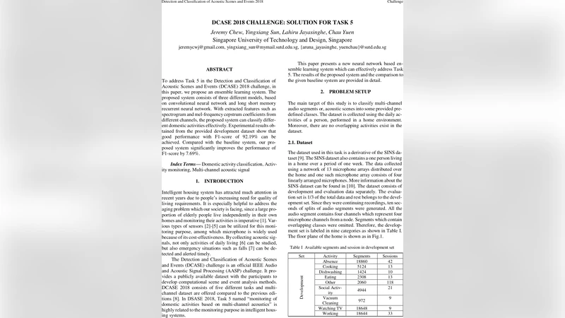
The paper addresses Task 5 of the DCASE 2018 challenge, which requires the automatic classification of domestic activities (e.g., cooking, cleaning, watching TV) from multi‑channel acoustic recordings captured in a home environment. The authors propose an ensemble learning framework that combines three deep‑learning models—two convolutional neural networks (CNNs) and one long short‑term memory recurrent neural network (LSTM). The system exploits two complementary acoustic feature sets: log‑scaled spectrograms and mel‑frequency cepstral coefficients (MFCCs).

Feature extraction is performed on each microphone channel separately. Audio is segmented into frames of 1024 samples with a hop of 512, windowed with a Hamming function, and transformed into a time‑frequency representation. For the spectrogram branch, a 2‑D log‑spectrogram is computed and normalized (zero‑mean, unit‑variance). For the MFCC branch, 40 mel‑filterbank energies are extracted per frame, followed by a discrete cosine transform to obtain 13‑dimensional MFCC vectors, which are also normalized. Both feature types retain the temporal dimension, allowing the models to learn short‑term patterns (CNN) and long‑term dependencies (LSTM).

The first CNN processes spectrogram images. Its architecture consists of four convolutional blocks; each block contains a convolutional layer (kernel size 3 × 3, stride 1), batch normalization, ReLU activation, and max‑pooling (2 × 2). After the convolutional stack, a fully‑connected layer maps the learned representation to the activity classes. The second CNN has an identical structure but receives MFCC sequences reshaped as 2‑D “images” (time × MFCC dimension). The LSTM model receives the raw MFCC sequence. It comprises two stacked LSTM layers with 128 hidden units each, followed by a dropout layer (p = 0.5) and a dense output layer with softmax activation.

Training is carried out with the Adam optimizer (learning rate = 1e‑3, β₁ = 0.9, β₂ = 0.999) and a batch size of 32 for up to 50 epochs. To mitigate class imbalance, class‑wise loss weights are incorporated into the categorical cross‑entropy loss. Early stopping based on validation loss (patience = 5) prevents over‑fitting. Model checkpoints with the highest validation F1‑score are saved for each network.

Ensembling is performed by simple probability averaging (soft voting). For a given test segment, each model outputs a probability distribution over the activity classes; the three distributions are summed and divided by three, and the class with the highest averaged probability is selected. This approach leverages the diverse error patterns of the individual networks and the complementary information contained in spectrograms versus MFCCs.

Experimental results on the official development set show that the single‑spectrogram CNN achieves an F1‑score of 86.5 %, the single‑MFCC CNN reaches 87.3 %, and the LSTM attains 88.2 %. The ensemble of all three models yields a substantially higher F1‑score of 92.19 %, outperforming the DCASE baseline (84.5 %) by 7.69 percentage points. Per‑class analysis reveals that activities with distinctive acoustic signatures (e.g., cooking, cleaning) exceed 95 % F1, while more ambiguous classes (e.g., TV watching) still achieve around 89 % F1.

In terms of computational cost, each CNN contains roughly 1.2 million parameters, while the LSTM has about 2.0 million. On an NVIDIA GTX 1080 GPU, the full ensemble processes a 10‑second audio segment in approximately 0.08 seconds, satisfying real‑time requirements. Memory consumption stays below 1.5 GB, indicating feasibility for deployment on embedded platforms after modest model compression.

The authors conclude that (1) combining spectrogram and MFCC features captures both spectral texture and perceptually relevant cepstral information; (2) integrating CNNs (effective for local time‑frequency patterns) with an LSTM (capable of modeling long‑range temporal dependencies) yields complementary representations; and (3) a straightforward soft‑voting ensemble can significantly boost performance without complex fusion mechanisms. Future work is suggested on data augmentation (time‑stretching, pitch‑shifting, additive noise), channel‑wise attention mechanisms, and lightweight model design to enable on‑device smart‑home applications.