Angular Softmax Loss for End-to-end Speaker Verification

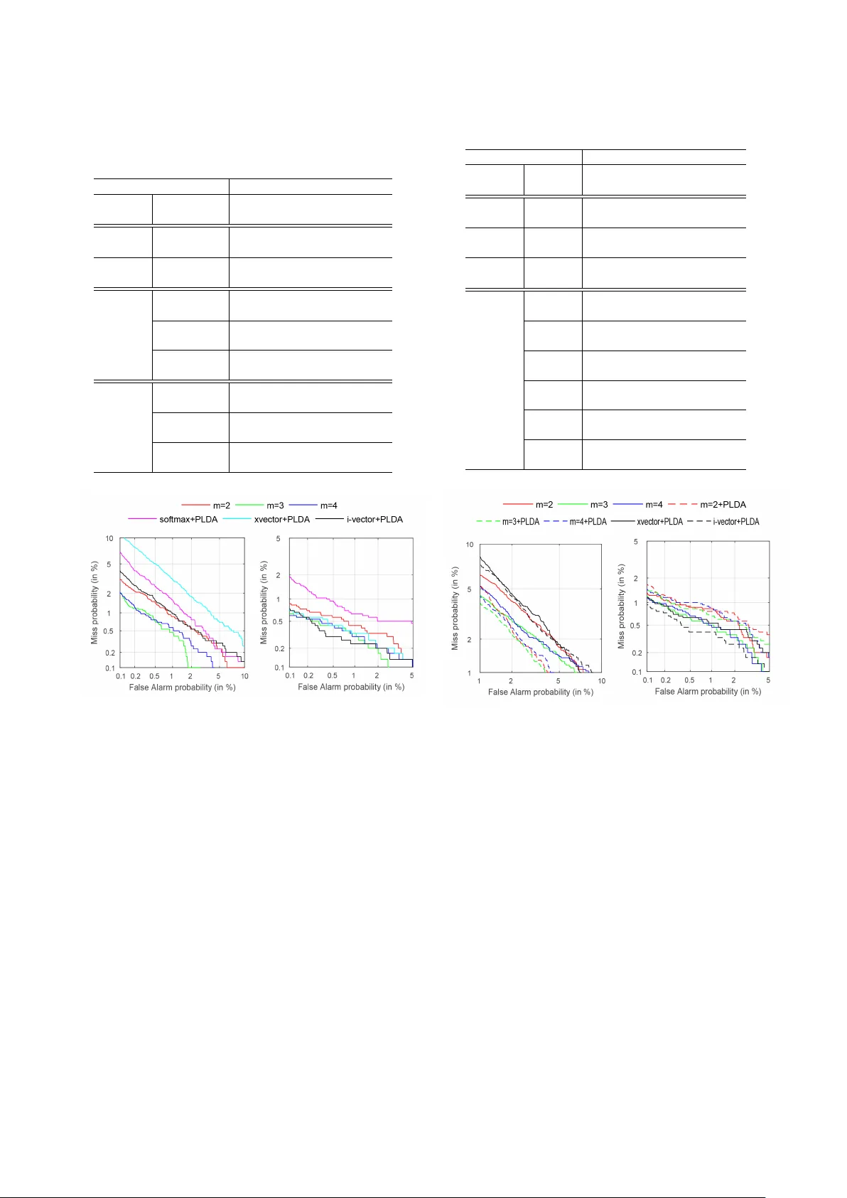
Angular Softmax Loss f or End-to-end Speaker V erification Y utian Li, F eng Gao, Zhijian Ou, Jiasong Sun Speech Processing and Machine Intelligence (SPMI) Lab, Tsinghua Uni versity , Beijing, China yutian-l16@mails.tsinghua.edu.cn, ozj@tsinghua.edu.cn Abstract End-to-end speaker verification systems hav e receiv ed increas- ing interests. The traditional i-vector approach trains a gen- erativ e model (basically a factor -analysis model) to e xtract i- vectors as speaker embeddings. In contrast, the end-to-end ap- proach directly trains a discriminativ e model (often a neural network) to learn discriminative speaker embeddings; a cru- cial component is the training criterion. In this paper , we use angular softmax (A-softmax), which is originally proposed for face verification, as the loss function for feature learning in end- to-end speak er v erification. By introducing margins between classes into softmax loss, A-softmax can learn more discrimi- nativ e features than softmax loss and triplet loss, and at the same time, is easy and stable for usage. W e make two contributions in this work. 1) W e introduce A-softmax loss into end-to-end speaker verification and achieve significant EER reductions. 2) W e find that the combination of using A-softmax in training the front-end and using PLD A in the back-end scoring further boosts the performance of end-to-end systems under short utter - ance condition (short in both enrollment and test). Experiments are conducted on part of F isher dataset and demonstrate the improv ements of using A-softmax. Index T erms : speaker verification, A-softmax, PLD A 1. Introduction Speaker verification is a classic task in speaker recognition, which is to determine whether two speech segments are from the same speaker or not. For man y years, most speaker verifica- tion systems are based on the i-vector approach [1]. The i-vector approach trains a generative model (basically a factor-analysis model) to extract i-vectors as speaker embeddings, and relies on v ariants of probabilistic linear discriminant analysis (PLD A) [2] for scoring in the back-end. End-to-end speaker verification systems hav e receiv ed in- creasing interests. The end-to-end approach directly trains a discriminativ e model (often a neural network) to learn discrim- inativ e speaker embeddings. V arious neural network structures hav e been explored. Some studies use RNNs to extract the iden- tity feature for an utterance [3][4][5][6][7]. Usually , the output at the last frame from the RNN is treated as the utterance-level speaker embedding. V arious attention mechanisms are also in- troduced to improve the performance of RNN-based speaker verification systems. There are also some studies based on CNNs [3][6][8][9][10], where the f-bank features are fed into the CNNs to model the patterns in the spectrograms. In addition to exploring different neural network architec- tures, an important problem in the end-to-end approach is to ex- plore dif ferent criteria (loss functions), which dri ve the network to learn discriminati ve features. In early studies, the features ex- tracted by the neural networks are fed into a softmax layer and This work is supported by NSFC grant 61473168. Correspondence to: Z. Ou (ozj@tsinghua.edu.cn). Speak er 1 Spe ak er 2 Spe ak er 3 Speak er n - 1 Spe ak er n …… …… …… …… …… …… …… …… …… F ea tur e e x tr act or Simila rity sc or e T r ain the model Ut t er anc es f or tr aining Ut t er anc es f or enr ollmen t Ut t er anc es f or t es ting …… …… …… (a) V erification task (b) Classification task Figure 1: Speech Utterances are r epr esented by small yellow blocks. Each row repr esents a speaker with a number of utter- ances. The above illustrates the verification task, which con- sists of feature extraction and scoring. The speakers used for training the feature extr actor usually do not appear in testing. The bottom shows the classification task. The speakers used for training the classifier appear in testing. Namely , in testing, ut- terances from the same set of training speakers are presented for classification. the cross entropy is used as the loss function. This loss is gener - ally referred to as “softmax loss”. But the softmax loss is more suitable for classification tasks (classifying samples into giv en classes). In contrast to classification, verification is an open- set task. Classes observed in the training set will generally not appear in the test set. Figure 1 shows the dif ference between the classification and verification tasks. A good loss for verifi- cation should push samples in the same class to be closer , and meanwhile drive samples from different classes further a way . In other w ords, we should make inter -class v ariances larger and intra-class variances smaller . A number of different loss func- tions hav e been proposed to address this problem [6][11][12]. T riplet loss [13] is recently proposed to take inter-class and intra-class variances into consideration. T riplet loss based train- ing requires a careful triplet selection procedure, which is both time-consuming and performance-sensitive. There are some in- teresting efforts to improve the triplet loss based training, such as generating triplets online from within a mini-batch [13], do- ing softmax pre-training [6]. Howe ver , training with the triplet loss remains to be a difficult task. Our experiment of using triplet loss yields inferior performance, compared to the i-vector method. Angular softmax (A-softmax) loss [14] is recently proposed to improve the softmax loss in face v erification. It enables end- to-end training of neural networks to learn angularly discrim- inativ e features. A-softmax loss introduces a margin between the tar get class and the non-target class into the softmax loss. The margin is controlled by a hyper-parameter m . The larger m is, the better the network will perform. Compared with the triplet loss, A-softmax is much easier to tune and monitor . In this paper , we introduce A-softmax loss into end-to-end speaker verification, as the loss function for learning speaker embeddings. In [14], cosine distance is used in the back-end scoring. Be yond of this, we study the combination of using A- softmax in training the front-end and using PLD A in the back- end scoring. Experiments are conducted on part of the F isher dataset. The neural network structure is similar to that used by the Kaldi xvector [15]. Using A-softmax performs signifi- cantly better than using softmax and triplet loss. The EERs of A-softmax system are the best on almost all conditions, except that both the enroll and the test utterances are long. It is known that the i-vector based system performs well under such long utterance condition [12, 8]. W e also find that under short utter- ance condition (short in both enrollment and test), using PLDA in the back-end can further reduce EERs of the A-softmax sys- tems. 2. Method A-softmax loss can be regarded as an enhanced v ersion of soft- max loss. The posterior probability giv en by softmax loss is: p i = e W T i x + b i P j e W T j x + b j where x is the input feature vector . W i and b i are the weight vector and bias in the softmax layer corresponding to class i , respectiv ely . T o illustrate A-softmax loss, we consider the two-class case. It is trivial to generalize the following analysis to multi- class cases. The posterior probabilities in the two-class case giv en by softmax loss are: p 1 = e W T 1 x + b 1 e W T 1 x + b 1 + e W T 2 x + b 2 p 2 = e W T 2 x + b 1 e W T 1 x + b 1 + e W T 2 x + b 2 The predicted label will be assigned to class 1 if p 1 ≥ p 2 and class 2 if p 1 < p 2 . The decision boundary is ( W T 1 − W T 2 ) x = 0 , which can be rewritten as ( k W 1 k cos( θ 1 ) − k W 2 k cos( θ 2 ) ) k x k = 0 . Here θ 1 , θ 2 are the angles between x and W 1 , W 2 respectiv ely . There are two steps of modifications in defining A-softmax [14]. First, when using cosine distance metric, it would be better to normalize the weights and and zero the biases, i.e. k W 1 k = k W 2 k = 1 and b 1 = b 2 = 0 . The decision boundary then be- comes angular boundary , as defined by cos( θ 1 ) − cos( θ 2 ) = 0 . Howe ver , the learned features are still not necessarily dis- criminativ e. Second, [14] further proposes to incorporate angu- lar margin to enhance the discrimination po wer . Specifically , an integer m ( m ≥ 2 ) is introduced to quantitatively con- trol the size of angular margin. The decision conditions for class 1 and class 2 become cos( mθ 1 ) − cos( θ 2 ) > 0 and cos( mθ 2 ) − cos( θ 1 ) > 0 respecti vely . This means when cos( mθ 1 ) > cos( θ 2 ) , we assign the sample to class 1; when cos( mθ 2 ) > cos( θ 1 ) , we assign the sample to class 2. Such decision conditions in A-softmax are more stringent than in the standard softmax. For example, to correctly clas- sify a sample x from class 1, A-softmax requires cos( mθ 1 ) > cos( θ 2 ) , which is stricter than cos( θ 1 ) > cos( θ 2 ) as required in the standard softmax. Because that the cosine function is monotonically decreasing in [0 , π ] , when θ 1 is in [0 , π m ] , we hav e cos( θ 1 ) > cos( mθ 1 ) > cos( θ 2 ) . It is shown in [14] that when all training samples are correctly classified according to A-softmax, the A-softmax decision conditions will produce an angular margin of m − 1 m +1 Θ , where Θ denotes the angle between W 1 and W 2 . By formulating the abo ve idea into the loss function, we obtain the A-softmax loss function for multi-class cases: L = 1 N N X n =1 − log e k x ( n ) k cos( mθ ( n ) y n ) e k x ( n ) k cos( mθ ( n ) y n ) + P j 6 = y n e k x ( n ) k cos( θ ( n ) j ) where N is the total number of training samples. x ( n ) and y ( n ) denote the input feature vector and the class label for the n -th training sample respectively . θ ( n ) j is the angle between x ( n ) and W j , and thus θ ( n ) y n denotes the angle between x ( n ) and the weight vector W y n . Note that in the above illustration, θ ( n ) y n is supposed to be in [0 , π m ] . T o remov e such restriction, a new function is defined to replace the cosine function as follows: φ ( θ ( n ) y n ) = ( − 1) k cos( mθ ( n ) y n ) − 2 k for θ ( n ) y n ∈ [ kπ m , ( k +1) π m ] and k ∈ [0 , m − 1] . So the A-softmax loss function is finally defined as follow: L = 1 N N X n =1 − log e k x ( n ) k φ ( θ ( n ) y n ) e k x ( n ) k φ ( θ ( n ) y n ) + P j 6 = y n e k x ( n ) k cos( θ ( n ) j ) By introducing m , A-Softmax loss adopts dif ferent deci- sion boundaries for different classes (each boundary is more stringent than the original), thus producing angular margin. The angular margin increases with lar ger m and would be zero if m = 1 . Compared with the standard softmax, A-softmax makes the decision boundary more stringent and separated, which can dri ve more discriminati ve feature learning. Com- pared with the triplet loss, using A-softmax loss do not need to sample triplets carefully to train the network. Using A-softmax loss in training is also straightfor- ward. During forward-propagation, we use normalized net- work weights. T o facilitate gradient computation and back- propagation, cos( θ ( n ) j ) and cos( mθ ( n ) y n ) can be replaced by ex- pressions only containing W and x ( n ) , according to the defi- nition of cosine and multi-angle formula 1 . In this manner, we can compute deriv ativ es with respect to W and x ( n ) , which is similar to using softmax loss in training. 1 That is the reason why we need m to be an integer . 3. Experimental Setup This section provides a description of our experimental setup including the data, acoustic features, baseline systems and the neural network architectures used in our end-to-end experi- ments. W e evaluate the traditional i-vector baseline and Kaldi xvector baseline [12, 15], which is an end-to-end speaker veri- fication system recently released as a part of Kaldi toolkit [16]. W e also conduct triplet loss experiments for comparison. 3.1. Data and acoustic features In our experiments, we randomly choose training and ev alu- ation data from F isher dataset, follo wing [8]. The training dataset consists of 5000 speakers randomly chosen from the F isher dataset, including 2500 male and 2500 female. This training dataset is used to train i-vector e xtractor , Kaldi xvector network, PLDA and our own network. The ev aluation dataset consists of 500 female and 500 male speakers randomly chosen from F isher dataset. There is no overlap in speakers between training and ev aluation data. The acoustic features are 23 dimensional MFCCs with a frame-length of 25ms. Mean-normalization over a sliding win- dow of up to 3 seconds is performed on each dimension of the MFCC features. And an energy-based V AD is used to detect speech frames. All experiments are conducted on the detected speech frames. 3.2. Baseline systems T wo baseline systems are e v aluated. The first baseline is a tradi- tional GMM-UBM i-v ector system, which is based on the Kaldi recipe. Delta and acceleration are appended to obtain 69 di- mensional feature vectors. The UBM is a 2048 component full- cov ariance GMM. The i-vector dimension is set to be 600. The second baseline is the Kaldi xvector system, which is detailed in the paper [15] and the Kaldi toolkit. W e use the de- fault setting in the Kaldi script. Basically , the system use a feed- forward deep neural network with a temporal pooling layer that aggregates over the input speech frames. This enables the net- work to be trained (based on the softmax loss) to extract a fix- dimensional speaker embedding vector (called xvector) from a varying-duration speech se gment. 3.3. PLD A back-end After extracting the speaker embedding vectors, we need a scor- ing module, or say a back-end, to make verification decision. Cosine distance and Euclidean distance are classic back-ends. Recently , likelihood-ratio score based back-ends such as PLD A (probabilistic linear discriminant analysis) have been shown to achiev e superior performance. In [17], PLD A and various re- lated models are compared. For consistent comparisons, Kaldi’ s implementation of PLD A, including length normalization but without LD A dimensionality reduction, is used in all PLD A- related experiments in this paper . 3.4. Our network ar chitecture Basically , we employ the same netw ork architecture to generate speaker embedding vectors as in Kaldi’ s xvector recipe. There are two minor differences in experiments. First, we do not use natural gradient descent [18] to optimize the network. Instead, we use the classic stochastic gradient descent. In our experi- ments, the minibatch size is 1000 chunks, and each chunk con- tains 200 speech frames. The learning rate is initialized as 0.01 T able 1: Details of our network ar chitectur e. Numbers in par en- theses denote the input and output dimensions in each layer . TDNN is time-delayed neural network. FC is fully connected neural network. utterance lev el layers FC 2 (512 → 300) FC 1 (3000 → 512) statistic pooling layer mean and standard deviation frame lev el layers TDNN 5 (512 × 1 → 1500) TDNN 4 (512 × 1 → 512) TDNN 3 (512 × 3 → 512) TDNN 2 (512 × 3 → 512) TDNN 1 (23 × 5 → 512) and then is multiplied by 0.9 after each epoch. The training stops when the learning rate drops to be below 0.0001, which roughly corresponds to 100 epochs of training. Second, we use ReLU layer [19] after batch normalization layer [20], which is found to be more stable in training than using the two layers in the opposite order as employed in the Kaldi xvector network. Details of our network architecture are sho wn in T able 1. 4. Experimental Results 4.1. Experiment with fixed-duration enroll utterances In the first experiment, we fix the durations of enroll utterances to be 3000 frames after V AD. The durations of test utterances vary in { 300 , 500 , 1000 , 1500 } frames after V AD. W e choose 1 enroll utterance and 3 test utterances per speak er from the ev al- uation dataset. T ogether we hav e 1 , 000 × 3 , 000 = 3 , 000 , 000 trials, which consist of 3 , 000 target trials and 2 , 997 , 000 non- target trials. The results are giv en in T able 2 and Figure 2, which shows the effect of different test durations on speaker verifica- tion performance in the long enrollment case. Some main observations are as follows. F irst , using triplet loss yields inferior performance. W e follo w the triplet sampling strategy in [7], which is also time consuming. Second , for short test condition (300 and 500 frames), A- softmax performs significantly better than both i-vector and xvector baseline. When testing with longer utterances (1500 frames), i-vector system performs better , which is also observed in [12, 8]. Similar observations can be seen from Figure 2, which shows the DET curves under 300 and 1500-frame test conditions. Thir d , to preclude the effect of the differences in network architecture in xvector system and our network, we can compare the results from softmax and A-softmax, both using our own network. A-softmax outperforms traditional softmax signifi- cantly . Compared to softmax with PLD A back-end, A-softmax with m = 3 and cosine back-end achie ves 48 . 46% , 58 . 76% , 47 . 14% and 41 . 10% EER relativ e reductions under 300, 500, 1000 and 1500-frame test conditions, respectiv ely . F orth , ideally , larger angular mar gin m could bring stronger discrimination power . In practice, this does not always hold due to the complication of neural network training, as seen from T able 2 and Figure 2. 4.2. Experiment with equal durations of enroll and test ut- terances In the second experiment, we set the durations of enroll and test utterances to be equal, v arying in { 300 , 500 , 1000 , 1500 } T able 2: EERs (%) for 3000-frame enr oll utterances and dif fer- ent durations of test utterances. m=2, 3, 4 ar e for A-softmax with m=2, 3, 4. Cosine is for cosine distance. Euclidean is for Euclidean distance. Durations of test utterances Model loss (metric) 300 500 1000 1500 iv ector - (PLD A) 1.00 0.53 0.33 0.37 xvector softmax (PLD A) 1.86 0.83 0.40 0.43 our network softmax (cosine) 1.67 1.17 0.90 0.83 softmax (PLD A) 1.30 0.97 0.70 0.73 triplet loss (Euclidean) 2.17 1.63 1.17 1.23 our network m = 2 (cosine) 0.94 0.60 0.47 0.57 m = 3 (cosine) 0.67 0.40 0.37 0.43 m = 4 (cosine) 0.70 0.47 0.33 0.47 Figure 2: DET curves with 3000-frame enr ollment, under 300- frame test condition (left) and 1500-frame test condition (right). The models can be our network ( m = 2 , 3 , 4 and “soft- max+PLD A ”), i-vector and xvector . frames after V AD. The trials are created, following the same strategy as in the first experiment. The results are given in T able 3 and Figure 3, which show the ef fect of dif ferent enroll and test durations on speaker verification performance. Some main observations are as follo ws. F irst , in this exper - iment, we add the results of A-softmax with PLD A back-end, which should be compared to A-softmax with cosine back-end. For short utterance condition (short in both enrollment and test, with 300 frames), using PLD A back-end significantly reduce EERs of the A-softmax systems. For m = 2 , 3 , 4 , the EER rel- ativ e reductions are 25 . 17% , 16 . 00% and 8 . 23% respectively . For long utterance condition (long in both enrollment and test), using PLDA back-end does not always improve the A-softmax systems. A possible reason is that during training, we slice the utterances into 200-frame chunks. Both the network and the PLD A are trained over 200-frame chunks, which consequently work best for short utterances. Second , we do not include the inferior result of triplet loss T able 3: EERs (%) with equal dur ations of enr oll and test utter- ances. Durations of utterances Model loss (metric) 300 500 1000 1500 iv ector - (PLD A) 2.93 1.57 0.50 0.47 xvector softmax (PLD A) 3.17 1.63 0.63 0.63 our network softmax (PLD A) 3.43 2.40 1.20 1.07 our network m = 2 (cosine) 2.90 1.57 0.77 0.83 m = 2 (PLD A) 2.17 1.33 0.73 0.80 m = 3 (cosine) 2.50 1.23 0.73 0.56 m = 3 (PLD A) 2.10 1.33 0.70 0.77 m = 4 (cosine) 2.43 1.33 0.70 0.63 m = 4 (PLD A) 2.23 1.37 0.73 0.90 Figure 3: DET curves with equal durations of enr oll and test, 300-frame condition (left) and 1500-fr ame condition (right). in T able 3. Compared to the i-vector and xvector baseline, the EERs of A-softmax system are the best on almost all condi- tions, e xcept that both the enroll and the test utterances are long (1000 and 1500 frames). This agree with the result in the first experiment and also in other papers [12, 8]. Thir d , when comparing softmax and A-softmax, both using our own network, A-softmax outperforms traditional softmax significantly on all conditions. 5. Conclusions In this work, we introduce A-softmax loss into end-to-end speaker verification, which outperforms softmax and triplet loss significantly , under the same neural network architecture. Fur- thermore, we use PLD A as back-end to impro ve A-softmax un- der short utterance condition. Compared with Kaldi i-vector baseline, A-softmax achieves better performance except for long utterance condition. 6. References [1] N. Dehak, P . J. Kenny , R. Dehak, P . Dumouchel, and P . Ouellet, “Front-end factor analysis for speaker verification, ” IEEE Tr ans- actions on A udio, Speech, and Language Pr ocessing , vol. 19, no. 4, pp. 788–798, 2011. [2] S. J. Prince and J. H. Elder, “Probabilistic linear discriminant anal- ysis for inferences about identity , ” in ICCV , 2007. [3] S.-X. Zhang, Z. Chen, Y . Zhao, J. Li, and Y . Gong, “End-to-end attention based te xt-dependent speaker v erification, ” in IEEE Spo- ken Language T echnology W orkshop (SLT) , 2016. [4] G. Heigold, I. Moreno, S. Bengio, and N. Shazeer, “End-to-end text-dependent speaker v erification, ” in ICASSP , 2016. [5] F . Chowdhury , Q. W ang, I. L. Moreno, and L. W an, “ Attention- based models for text-dependent speaker verification, ” arXiv pr eprint arXiv:1710.10470 , 2017. [6] C. Li, X. Ma, B. Jiang, X. Li, X. Zhang, X. Liu, Y . Cao, A. Kan- nan, and Z. Zhu, “Deep speaker: an end-to-end neural speaker embedding system, ” arXiv preprint , 2017. [7] H. Bredin, “Tristounet: triplet loss for speaker turn embedding, ” in ICASSP , 2017. [8] L. Li, Y . Chen, Y . Shi, Z. T ang, and D. W ang, “Deep speaker feature learning for text-independent speaker verification, ” in In- terspeech , 2017. [9] A. T orfi, N. M. Nasrabadi, and J. Dawson, “T ext-independent speaker verification using 3d conv olutional neural networks, ” in IEEE International Conference on Multimedia and Expo (ICME) , 2017. [10] C. Zhang and K. Koishida, “End-to-end te xt-independent speaker verification with triplet loss on short utterances, ” in Interspeech , 2017. [11] L. W an, Q. W ang, A. Papir , and I. L. Moreno, “General- ized end-to-end loss for speak er verification, ” arXiv preprint arXiv:1710.10467 , 2017. [12] D. Snyder, P . Ghahremani, D. Pove y , D. Garcia-Romero, Y . Carmiel, and S. Khudanpur, “Deep neural network-based speaker embeddings for end-to-end speaker verification, ” in IEEE Spoken Language T echnology W orkshop (SLT) , 2016. [13] F . Schroff, D. Kalenichenko, and J. Philbin, “Facenet: A unified embedding for face recognition and clustering, ” in IEEE Confer- ence on Computer V ision and P attern Recognition (CVPR) , 2015. [14] W . Liu, Y . W en, Z. Y u, M. Li, B. Raj, and L. Song, “Sphereface: Deep h ypersphere embedding for face recognition, ” in IEEE Con- fer ence on Computer V ision and P attern Recognition (CVPR) , 2017. [15] D. Snyder , D. Garcia-Romero, D. Povey , and S. Khudanpur , “Deep neural network embeddings for text-independent speaker verification, ” in Interspeech , 2017. [16] D. Po vey , A. Ghoshal, G. Boulianne, L. Bur get, O. Glembek, N. Goel, M. Hannemann, P . Motlicek, Y . Qian, P . Schwarz, J. Silovsky , G. Stemmer , and K. V esely , “The kaldi speech recog- nition toolkit, ” in IEEE W orkshop on Automatic Speech Recogni- tion and Understanding (ASR U) , 2011. [17] Y . W ang, H. Xu, and Z. Ou, “Joint bayesian gaussian discriminant analysis for speaker verification, ” in ICASSP , 2017. [18] D. Pove y , X. Zhang, and S. Khudanpur, “Parallel training of deep neural networks with natural gradient and parameter averaging, ” in ICLR , 2014. [19] X. Glorot, A. Bordes, and Y . Bengio, “Deep sparse rectifier neural networks, ” in AIST A TS , 2011. [20] S. Iof fe and C. Szegedy , “Batch normalization: Accelerating deep network training by reducing internal covariate shift, ” in ICML , 2015.