Highway Long Short-Term Memory RNNs for Distant Speech Recognition

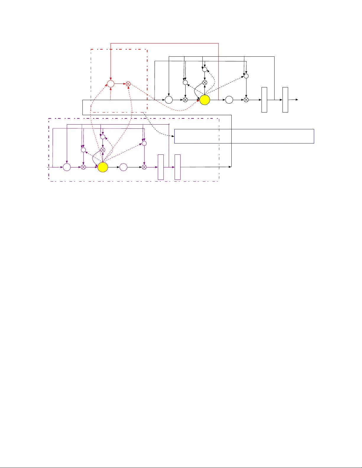
HIGHW A Y LONG SHOR T -TERM MEMOR Y RNNS FOR DIST ANT SPEECH RECOGNITION Y u Zhang 1 , Guoguo Chen 2 , Dong Y u 3 , Kaisheng Y ao 3 , Sanjeev Khudanpur 2 , James Glass 1 ∗ 1 MIT CSAIL 2 JHU CLSP 3 Microsoft Research { yzhang87,glass } @mit.edu, { guoguo,khudanpur } @jhu.edu, { dongyu, Kaisheng.YAO } @microsoft.com ABSTRA CT In this paper , we extend the deep long short-term memory (DL- STM) recurrent neural networks by introducing gated direct con- nections between memory cells in adjacent layers. These direct links, called highway connections, enable unimpeded information flow across different layers and thus alle viate the gradient vanish- ing problem when building deeper LSTMs. W e further introduce the latency-controlled bidirectional LSTMs (BLSTMs) which can exploit the whole history while keeping the latency under control. Efficient algorithms are proposed to train these novel networks us- ing both frame and sequence discriminati ve criteria. Experiments on the AMI distant speech recognition (DSR) task indicate that we can train deeper LSTMs and achie ve better improv ement from sequence training with highw ay LSTMs (HLSTMs). Our nov el model obtains 43 . 9 / 47 . 7% WER on AMI (SDM) dev and ev al sets, outperforming all previous works. It beats the strong DNN and DLSTM baselines with 15 . 7% and 5 . 3% relative impro vement respecti vely . Index T erms — Highway LSTM, CNTK, LSTM, Sequence T raining 1. INTR ODUCTION Recently the deep neural network (DNN)-based acoustic models (AMs) greatly improved automatic speech recognition (ASR) accu- racy on many tasks [1, 2, 3, 4]. Further improvements were reported by using more advanced models such as con volutional neural net- works (CNNs) [5] and long short-term memory (LSTM) recurrent neural networks (RNNs) [6, 7, 8]. Although these new techniques help to decrease the word error rate (WER) on distant speech recognition (DSR) [9], DSR remains a challenging task due to the rev erberation and overlapping acoustic signals, even with sophisticated front-end processing techniques [10, 11, 12] and multi-pass decoding schemes. In this paper , we explore more adv anced back-end techniques for DSR. It is reported [8] that deep LSTM (DLSTM) RNNs help improv e generalization and often outperform single-layer LSTM RNNs. Howe ver , DLSTM RNNs are harder to train and slo wer to con ver ge. In this paper , we extend DLSTM RNNs by introducing a gated direct connection between memory cells of adjacent layers. These direct links, called highway connections, provide a path for information to flo w between layers more directly without decay . It alleviates the gradient vanishing problem and enables DLSTM RNNs training with virtually arbitrary depth. Here, we refer to an LSTM RNN with highway connections as HLSTM RNN. ∗ Part of the work reported here was carried out during the 2015 Jelinek Memorial Summer W orkshop on Speech and Language T echnologies at the Univ ersity of W ashington, Seattle, and was supported by Johns Hopkins Uni- versity via NSF Grant No IIS 1005411, and gifts from Google, Microsoft Research, Amazon, Mitsubishi Electric, and MERL. T o further improv e the performance, we also introduce the latency-controlled bidirectional LSTM (LC-BLSTM) RNNs. In the LC-BLSTM RNNs, the past history is fully exploited similar to that in the unidirectional LSTM RNNs. Ho wev er , unlike the standard BLSTM RNNs which can start model e valuation only af- ter seeing the whole utterance, the LC-BLSTM RNNs only look ahead for a fixed number of frames which limits the latency . The LC-BLSTM can be much more efficiently trained than the standard BLSTM without performance loss. It also trains and decodes faster than conte xt-sensitiv e-chunk BLSTMs [13] which can only access limited past and future context. Our study is conducted on the AMI single distant microphone (SDM) setup. W e compare the standard (B)LSTM RNNs and high- way (B)LSTM RNNs with 3 and 8 layers. W e show that the highway (B)LSTM RNNs with dropout applied to the highway connection significantly outperform the standard (B)LSTM RNNs. The high way connection helps to train deeper networks better and the high- way (B)LSTM RNNs seem to benefit more from sequence discrim- inativ e training. Ov erall, our proposed model decreased WER by 15 . 7% ov er DNNs, 14 . 4% over CNNs [14], and 5 . 3% over DLSTM RNNs relatively . T o our best knowledge, the 43 . 9 / 47 . 7% WER we achiev ed on the AMI (SDM) dev and ev al sets is the best results reported on this task. 1 . The rest of the paper is organized as follows. In Section 2 we briefly discuss related w ork. In Section 3 we introduce standard DL- STM RNNs, BLSTM RNNs, and the highway (B)LSTM RNNs. In Section 4 we describe LC-BLSTM and the way to train such mod- els efficiently with both frame and sequence discriminativ e criteria. W e summarize the experimental setup in Section 5 and report exper- imental results in Section 6. Conclusions are reiterated in Section 7. 2. RELA TED WORK After dev eloping the highway LSTMs independently we noticed that similar work has been done in [16, 17, 18]. All of these works share the same idea of adding gated linear connections between different layers. The highway networks proposed in [16] adaptiv ely carry some dimensions of the input directly to the output so that infor- mation can flow across layers much more easily . Ho wev er , their formulation is different from ours and their focus is DNN. The work in [17] share the same idea and model structure. [18] is more general and uses a generic form. Ho wev er , their task is on text e.g. machine translation while our focus is distant speech recognition. In addi- tion, we used dropout as the w ay to control the highway connections which turns out to be critical for DSR. 1 The tools and scripts used to produce the results reported in this paper are publicly av ailable as part of the CNTK toolkit[15], and anyone with access to the data should be able to reproduce our results. cell g recurrent output cell g h i ( l +1) t f ( l +1) t o ( l +1) t recurrent output r ( l +1) t r ( l +1) t  1 m ( l +1) t y ( l +1) t d ( l +1) t c ( l ) t c ( l +1) t  1 c ( l ) t  c ( l +1) t l l +1 x ( l +1) t d ( l +1) t =  ( b ( l +1) d + W ( l +1) xd x ( l +1) t + w ( l +1) cd  c ( l +1) t  1 + w ld  c l t ) Highway Block LSTM Block h Fig. 1 . Highway Long Short-T erm Memory RNNs 3. HIGHW A Y LONG SHOR T -TERM MEMOR Y RNNS 3.1. Long short-term memory RNNs The LSTM RNN was initially proposed in [19] to solve the gradient diminishing problem in RNNs. It introduces a linear dependence between c t , the memory cell state at time t , and c t − 1 , the same cell’ s state at t − 1 . Nonlinear gates are introduced to control the information flo w . The operation of the network follows the equations i t = σ ( W xi x t + W mi h t − 1 + W ci c t − 1 + b i ) (1) f t = σ ( W xf x t + W mf h t − 1 + W cf c t − 1 + b f ) (2) c t = f t  c t − 1 + i t  tanh( W xc x t + W mc m t − 1 + b c ) (3) o t = σ ( W xo x t + W mo h t − 1 + W co c t + b o ) (4) m t = o t  tanh( c t ) (5) iterativ ely from t = 1 to T , where σ ( ˙ ) is the logistic sigmoid func- tion, i t , f t , o t , c t and m t are vectors to represent v alues at time t of the input gate, forget gate, output gate, cell activ ation, and cell output activ ation respectively .  denotes element-wise product of vectors. W ∗ are the weight matrices connecting different gates, and b ∗ are the corresponding bias vectors. All the matrices are full except the matrices W ci , W cf , W co from the cell to gate vector which is di- agonal. 3.2. Deep LSTM RNNs Deep LSTM RNNs are formed by stacking multiple layers of LSTM cells. Specifically , the output of the lower layer LSTM cells y l t is fed to the upper layer as input x l +1 t . Although each LSTM layer is deep in time since it can be unrolled in time to become a feed- forward neural network in which each layer shares the same weights, deep LSTM RNNs still outperform single-layer LSTM RNNs signif- icantly . It is conjectured [8] that DLSTM RNNs can make better use of parameters by distributing them ov er the space through multiple layers. Note that in the con ventional DLSTM RNNs the interaction between cells in dif ferent layers must go through the output-input connection. 3.3. HLSTM RNNs The Highw ay LSTM (HLSTM) RNN proposed in this paper is illus- trated in Figure 1. It has a direct gated connection (in the red block) between the memory cells c l t in the lo wer layer l and the memory cells c l +1 t in the upper layer l + 1 . The carry gate controls how much information can flo w from the lower -layer cells directly to the upper-layer cells. The gate function at layer l + 1 at time t is d ( l +1) t = σ ( b ( l +1) d + W l +1 xd x ( l +1) t + w l +1 cd  c ( l +1) t − 1 + w ( l +1) ld  c l t ) , (6) where b ( l +1) d is a bias term, W ( l +1) xd is the weight matrix connecting the carry gate to the input of this layer . w ( L +1) cd is a weight vector from the carry gate to the past cell state in the current layer . w ( L +1) ld is a weight vector connecting the carry gate to the lower layer mem- ory cell. d ( l +1) is the carry gate acti vation v ectors at layer l + 1 . Using the carry gate, an HLSTM RNN computes the cell state at layer ( l + 1) according to c l +1 t = d ( l +1) t  c l t + f ( l +1) t  c ( l +1) t − 1 + i ( l +1) t  tanh( W ( l +1) xc x ( l +1) t + W ( l +1) hc m ( l +1) t − 1 + b c ) , (7) while all other equations are the same as that in the standard LSTM RNNs as described in Eq. (1),(2),(4), and (5). Thus, depending on the output of the carry gates, the highway connection can smoothly v ary its behavior between that of a plain LSTM layer or simply passes its cell memory from previous layer . The highway connection between cells in dif ferent layers makes in- fluence from cells in one layer to the other more direct and can al- leviate the gradient vanishing problem when training deeper LSTM RNNs. 3.4. Bidirectional Highway LSTM RNNs The unidirectional LSTM RNNs we described above can only ex- ploit past history . In speech recognition, howe ver , future contexts also carry information and should be utilized to further enhance acoustic models. The bidirectional RNNs take advantage of both past and future contexts by processing the data in both directions with two separate hidden layers. It is shown in [6, 7, 13] that bidi- rectional LSTN RNNs can indeed improve the speech recognition results. In this study , we also extend the HLSTM RNNs from unidi- rection to bidirection. Note that the backward layer follo ws the same equations used in the forward layer except that t − 1 is replaced by t + 1 to exploit future frames and the model operates from t = T to 1 . The output of the forward and backward layers are concatenated to form the input to the next layer . 4. EFFICIENT NETWORK TRAINING Now adays, GPUs are widely used in deep learning by lev erag- ing massive parallel computations via mini-batch based training. For unidirectional RNN models, to better utilize the parallelization power of the GPU card, in [15], multiple sequences (e.g., 40) are often packed into the same mini-batch. Truncated BPTT is usually performed for parameters updating, therefore, only a small segment (e.g., 20 frames) of each sequence has to be packed into the mini- batch. Howe ver , when applied to sequence lev el training (BLSTM or sequence training), GPU’ s limited memory restricts the number of sequences that can be packed into a mini-batch, especially for L VCSR tasks with long training sequences and large model sizes. One alternative way to speed up is using asynchronous SGD based on a GPU/CPU farm [20]. In this section, we are more focused on fully utilizing the parallelization power of a single GPU Card. The algorithms proposed here can also be applied to a multi-GPU setup. 4.1. Latency-controlled bi-directional model training T o speed up the training of bi-direcctional RNNs, the Context- sensitiv e-chunk BPTT (CSC-BPTT) is proposed in [13]. In this method, a sequence is firstly split into chunks of fixed length N c . Then N l past frames and N r future frames are concatenated before and after each chunk as the left and right context, respecti vely . The appended frames are only used to pro vide context information and do not generate error signals during training. Since each trunk can be independently drawn and trained, they can be stacked to form large minibatches to speed up training. Unfortunately , the model trained with CSC-BPTT is no longer the true bidirectional RNN since the history it can exploit is limited by the left and right context concatenated to the chunk. It also in- troduces additional computation cost during decoding since both the left and right contexts need to be recomputed for each chunk. T o solve the problems in the CSC-BPTT we propose the latency- controlled bi-directional RNNs. Different from the CSC-BPTT , in our ne w model we carry the whole past history while still using a truncated future context. Instead of concatenating and computing N l left contextual frames for each chunk we directly carry over the left contextual information from the previous chunk of the same ut- terance. For e very chunk, both training and decoding computational cost is reduced by a factor of N l N l + N c + N r . Moreov er , loading the history from previous mini-batch instead of a fixed contextual win- dows mak es the context exact when compared to the uni-directional model. Note that the standard BLSTM RNNs come with significant latency since the model can only be e valuated after seeing the whole utterance. In the latency-controlled BLSTM RNNs the latency is limited to N r which can be set by the users. In our experiments, we process 40 utterances in parallel which is 10 times f aster than pro- cessing the whole utterances without performance loss. Compared to the CSC BPTT our approach is 1.5 times faster and often leads to better accuracy . 4.2. T wo pass forward computation for sequence training T o increase the number of sequences that can be fit into a mini-batch, we propose a two-forward-pass solution for sequence discriminati ve training on top of recurrent neural netw orks. The basic idea is pretty straightforward. For sequence training of recurrent models, we use the same mini-batch packaging method as that in the cross-entropy training case, i.e., we pack multiple sequences (e.g., 40) into the same mini-batch, each with a small chunk (e.g., 20 frames). Then in the first forward pass, we collect log-likelihood of frames in the mini-batch, and put those into a pool, without updating the model. W e do this until we hav e collected the log-likelihood for a certain number of sequences. At this point, we are able to compute the error signal for each of the sequence in the pool. W e then roll back the mini-batches that we hav e just computed error signals for, and start the second forward pass, this time we update the model using the error signals from the pool. With this two-forward-pass solution, we are able to pack far more sequences in the same mini-batch, e.g., 40 ∼ 60, thus leading to much faster training. 5. EXPERIMENT SETUP 5.1. Corpus W e ev aluated our models on the AMI meeting corpus [21]. The AMI corpus comprises around 100 hours of meeting recordings, recorded in instrumented meeting rooms. Multiple microphones were used, including individual headset microphones (IHM), lapel microphones, and one or more microphone arrays. In this work, we use the single distant microphone (SDM) condition for our experiments. Our systems are trained and tested using the split recommended in the corpus release: a training set of 80 hours, a dev elopment set and a test set each of 9 hours. For our training, we use all the se gments provided by the corpus, including those with ov erlapped speech. Our models are ev aluated on the ev aluation set only . NIST’ s asclite tool [22] is used for scoring. 5.2. System description Kaldi [23] is used for feature extraction, early stage triphone training as well as decoding. A maximum likelihood acoustic training recipe is used to trains a GMM-HMM triphone system. Forced alignment is performed on the training data by this triphone system to generate labels for further neural network training. The Computational Network T oolkit (CNTK) [15] is used for neural network training. W e start off by training a 6-layer DNN, with 2 , 048 sigmoid units per layer . 40-dimensional filterbank fea- tures, together with their corresponding delta and delta-delta features are used as raw feature vectors. For our DNN training we concate- nated 15 frames of raw feature vectors, which leads to a dimension of 1 , 800 . This DNN again is used to force align the training data to generate labels for further LSTM training. Our (H)LSTM models, unless explicitly stated otherwise, are added with a projection layer on top of each layer’ s output, as pro- posed in [8], and are trained with 80-dimensional log Mel filterbank (FB ANK) features. For LSTMP models, each hidden layer consists of 1024 memory cells together with a 512-node projection layer . For the BLSTMP models, each hidden layer consists of 1024 memory cells (512 for forward and 512 for backward) with a 300-node pro- jection layer . Their highway companions share the same network structure, except the additional highway connections. All models are randomly initialized without either generativ e or discriminativ e pretraining [24]. A v alidation set is used to control the learning rate which will be halved when no gain is observed. T o train the unidirectional model, the truncated back-propagation- through-time (BPTT) [25] is used to update the model parameters. Each BPTT segment contains 20 frames and process 40 utterances simultaneously . T o train the latency-controlled bidirectional model, we set N c = 22 and N r = 21 and also process 40 utterances si- multaneously . A start learning rate of 0.2 per minibatch is used and then the learning rate scheduler tak es action. For frame level cross-entropy training, L 2 constraint regularization [26] is used. For sequence training, L 2 constraint re gularization is also applied when- ev er it is used in the corresponding cross-entrop y trained model. W e use a fixed per sample learning rate of 1 e − 5 for DNN sequence training, and 2 e − 6 for LSTM sequence training. 6. RESUL TS The performance of various models are ev aluated using word error rate (WER) in percent below . All the experiments are conducted on AMI SDM1 ev al set, if not specified otherwise. Since we do not exclude the overlapping speech segments during model training, in addition to results on the full eval set, we also show results on a subset that only contains the non-overlapping speech segments as [14]. 6.1. 3-layer Highway (B)LSTMP System #Layers with ov erlap no overlap DNN 6 57.5 48.4 LSTMP 3 50.7 41.7 HLSTMP 3 50.4 41.2 BLSTMP 3 48.5 38.9 BHLSTMP 3 48.3 38.5 T able 1 . Performance of highway (B)LSTMP RNNs T able 1 gives WER performance of the 3-layer LSTMP and BLSTMP RNNs, as well as their highway versions. The perfor- mance of the DNN network is also listed for comparison. From the table, it’ s clear that the highway version of the LSTM RNNs con- sistently outperform their non-highway companions, though with a small margin. 6.2. Highway (B)LSTMP with dr opout System #Layers with ov erlap no overlap LSTMP 3 50.7 41.7 HLSTMP + dropout 3 49.7 40.5 BLSTMP 3 48.5 38.9 BHLSTMP + dropout 3 47.5 37.9 T able 2 . Performance of highway (B)LSTMP RNNs with dropout Dropout is applied to the highway connection to control its flow: a high dropout rate essentially turns off the highw ay connection, and a small dropout rate, on the other hand, keeps the connection aliv e. In our experiments, for early training stages, we use a small dropout rate of 0 . 1 , and increase it to 0 . 8 after 5 epochs of training. Per- formance of highway (B)LSTMP networks with dropout is sho wn in T able 2, as we can see, dropout helps to further bring do wn the WER for highway networks. 6.3. Deeper highway LSTMP System #layers with ov erlap no overlap LSTMP 3 50.7 41.7 LSTMP 8 52.6 43.8 HLSTMP 3 50.4 41.2 HLSTMP 8 50.7 41.3 T able 3 . Comparison of shallow and deep networks When a network goes deeper, the training usually becomes dif- ficult. T able 3 compares the performance of shallow and deep net- works. From the table we can see that for a normal LSTMP network, when it goes from 3 layers to 8 layers, the recognition performance degrades dramatically . For the highway network, ho wev er , the WER only increase a little bit. The table suggests that the highway con- nection between LSTM layers allo ws the netw ork to go much deeper than the normal LSTM networks. 6.4. Highway LSTMP with sequence training System (dr: dropout) #Layers with overlap no o verlap DNN 6 57.5 48.4 DNN + sMBR 6 54.4 44.7 LSTMP 3 50.7 41.7 LSTMP + sMBR 3 49.3 39.8 HLSTMP 3 50.4 41.2 HLSTMP + sMBR 3 48.3 38.4 HLSTMP (dr) + sMBR 3 47.7 38.2 LSTMP 8 52.6 43.8 LSTMP + sMBRR 8 50.5 41.3 HLSTMP 8 50.7 41.3 HLSTMP + sMBR 8 47.9 37.7 T able 4 . Performance of sequence training on various networks W e perform sequence discriminati ve training for the networks discussed in Section 4.2. Detailed results are shown in T able 4. The table suggests that introducing the highway connection between LSTMP layers is beneficial to sequence discriminati ve training. F or example, without the highway connection, sequence training on top of the 3-layer LSTMP netw ork brings WER from 50 . 7 down to 49 . 3 , a relative improvement of only 3% on this particular task. After in- troducing the highway connection and dropout, the improvement is from 50 . 4 to 47 . 7 , 5% relativ ely . The relative improvement is even larger on the non-overlapping segment subset, which is roughly 7% . The results suggest that sequence training is beneficial from both highway connection and a deeper structure. 7. CONCLUSION W e presented a nov el highway LSTM network, and applied it to a far -field speech recognition task. Experimental results suggest that this type of network consistently outperforms the normal (B)LSTMP networks, especially when dropout is applied to the highway con- nection to control the connection’ s on/off state. Further experiments also suggest that the highway connection allows the network to go much deeper , and to get larger benefit from sequence discriminative training. 8. REFERENCES [1] G. E. Dahl, D. Y u, L. Deng, and A. Acero, “Context-dependent pre-trained deep neural networks for lar ge-vocab ulary speech recognition, ” IEEE T ransactions on Audio, Speech and Lan- guage Pr ocessing , vol. 20, no. 1, pp. 30–42, 2012. [2] F . Seide, G. Li, and D. Y u, “Con versational speech transcrip- tion using context-dependent deep neural networks, ” in Proc. Annual Conference of International Speech Communication Association (INTERSPEECH) , 2011, pp. 437–440. [3] G. Hinton, L. Deng, D. Y u, G. Dahl, A. Mohamed, N. Jaitly , A. Senior , V . V anhoucke, P . Nguyen, T . Sainath, and B. Kings- bury , “Deep neural networks for acoustic modeling in speech recognition: The shared vie ws of four research groups, ” IEEE Signal Pr ocessing Magazine , no. 6, pp. 82–97, 2012. [4] M. Seltzer , D. Y u, and Y . Q. W ang, “ An inv estigation of deep neural networks for noise robust speech recognition, ” in Pr oc. International Confer ence on Acoustics, Speech and Signal Pr o- cessing (ICASSP) , 2013. [5] P . Swietojanski, A. Ghoshal, and S. Renals, “Con volutional neural networks for distant speech recognition, ” Signal Pr o- cessing Letters, IEEE , vol. 21, no. 9, pp. 1120–1124, Septem- ber 2014. [6] A. Graves, A. Mohamed, and G. Hinton, “Speech recogni- tion with deep recurrent neural networks, ” in Pr oc. Interna- tional Confer ence on Acoustics, Speech and Signal Pr ocessing (ICASSP) , 2013. [7] A. Grav es, N. Jaitly , and A. Mohamed, “Hybrid speech recog- nition with deep bidirectional LSTM, ” in Proc. IEEE W orkshop on Automfatic Speech Recognition and Understanding (ASR U) , 2013, pp. 273–278. [8] H. Sak, A. Senior, and F . Beaufays, “Long short-term memory recurrent neural network architectures for large scale acoustic modeling, ” in Fifteenth Annual Confer ence of the International Speech Communication Association , 2014. [9] P . Swietojanski, A. Ghoshal, and S. Renals, “Hybrid acoustic models for distant and multichannel large v ocabulary speech recognition, ” in ASR U , 2013. [10] K. Kumatani, J. W . McDonough, and B. Raj, “Microphone array processing for distant speech recognition: From close- talking microphones to far -field sensors. ” IEEE Signal Process. Mag. , v ol. 29, no. 6, pp. 127–140, 2012. [11] T . Hain, L. Burget, J. Dines, P . N. Garner , F . Grzl, A. E. Hannani, M. Huijbregts, M. Karafit, M. Lincoln, and V . W an, “T ranscribing meetings with the amida systems. ” IEEE T rans- actions on Audio, Speech & Language Processing , vol. 20, no. 2, pp. 486–498, 2012. [12] A. Stolcke, “Making the most from multiple microphones in meeting recognition, ” in ICASSP , 2011. [13] K. Chen, Z.-J. Y an, and Q. Huo, “Training deep bidirectional lstm acoustic model for lvcsr by a conte xt-sensitiv e-chunk bptt approach, ” in Interspeech , 2015. [14] P . Swietojanski, A. Ghoshal, and S. Renals, “Con volutional neural networks for distant speech recognition, ” IEEE Singal Pr ocessing Letters , vol. 21, no. 9, pp. 1120–1124, 2014. [15] D. Y u, A. Eversole, M. Seltzer , K. Y ao, B. Guenter, O. Kuchaie v , Y . Zhang, F . Seide, G. Chen, H. W ang, J. Droppo, A. Ag arwal, C. Basoglu, M. Padmilac, A. Kamenev , V . Iv anov , S. Cyphers, H. Parthasarathi, B. Mitra, Z. Huang, G. Zweig, C. Rossbach, J. Currey , J. Gao, A. May , B. Peng, A. Stolcke, M. Slaney , and X. Huang, “ An introduction to computational networks and the computational network toolkit, ” Microsoft T echnical Report , 2014. [16] R. Sriv astav a, K. Greff, and J. Schmidhuber , “Highw ay networks, ” 2015. [Online]. A vailable: http://arxiv .or g/abs/ 1505.00387 [17] K. Y ao, T . Cohn, K. Vylomova, K. Duh, and C. Dyer, “Depth-gated lstm, ” 2015. [Online]. A vailable: http://arxi v . org/abs/1508.03790 [18] N. Kalchbrenner , I. Danihelka, and A. Graves, “Grid long short-term memory , ” 2015. [Online]. A vailable: http: //arXiv .or g/abs/1507.01526 [19] S. Hochreiter and J. Schmidhuber , “Long short-term memory , ” Neural Computation , vol. 9, no. 8, p. 17351438, 1997. [20] G. Heigold, E. McDermott, V . V anhoucke, A. Senior , and M. Bacchiani, “ Asynchronous stochastic optimization for se- quence training of deep neural networks, ” in ICASSP , 2014. [21] J. Carletta, “unleashing the killer corpus: experiences in cre- ating the multi-e verything ami meeting corpus, ” Language Re- sour ces & Evaluation Journal , vol. 41, no. 2, pp. 181–190, 2007. [22] J. Fiscus, J. Ajot, N. Radde, and C. Laprun, “Multiple dimen- sion lev enshtein edit distance calculations for ev aluating asr systems during simultaneous speech, ” in LREC , 2006. [23] D. Pove y , A. Ghoshal, G. Boulianne, L. Burget, O. Glembek, N. Goel, M. Hannemann, P . Motl ´ ı ˇ cek, Y . Qian, P . Schwarz, J. Silovsk ´ y, G. Stemmer, and K. V esel ´ y, “The Kaldi speech recognition toolkit, ” in ASR U , 2011. [24] F . Seide, G. Li, X. Chen, and D. Y u, “Feature engineering in context-dependent deep neural networks for conv ersational speech transcription, ” in Pr oc. IEEE W orkshop on Automfatic Speech Recognition and Understanding (ASR U) , 2011, pp. 24– 29. [25] R. W illiams and J. Peng, “ An efficient gradient-based algo- rithm for online training of recurrent network trajectories, ” Neural Computation , vol. 2, p. 490501, 1990. [26] G. E. Hinton, N. Sriv astav a, A. Krizhevsky , I. Sutskever , and R. Salakhutdinov , “Improving neural networks by preventing co-adaptation of feature detectors, ” 2012. [Online]. A vailable: http://arxiv .or g/abs/1207.0580