Variational Bayes In Private Settings (VIPS)

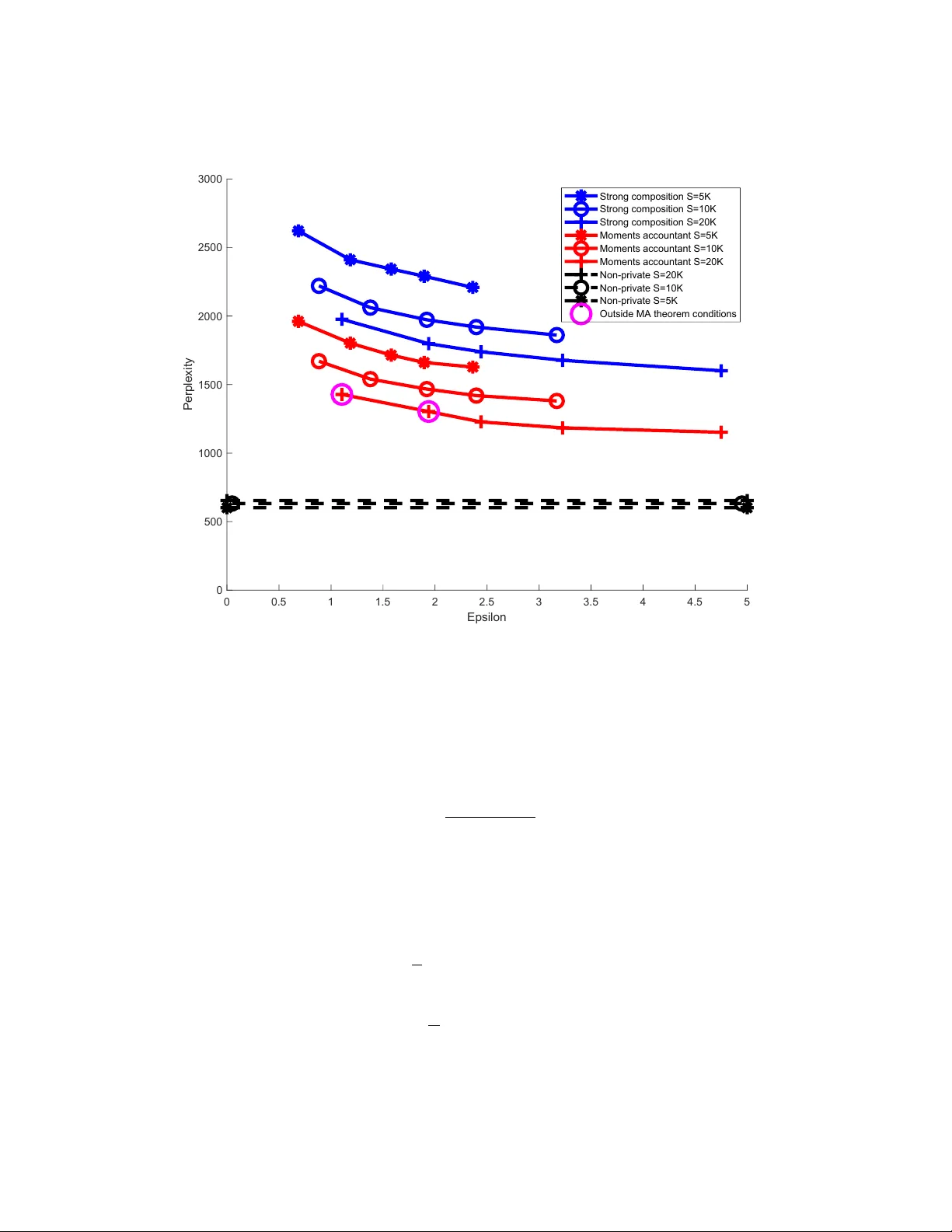
V ariational Ba y es In Priv ate Settings (VIPS) Mijung P ark mijungi.p@gmail.com Max Planck Institute for Intel ligent Systems & University of T¨ ubingen Max-Planck-R ing 4, 72076 T ¨ ubingen, Germany James F oulds jfoulds@umbc.edu Dep artment of Information Systems, University of Maryland, Baltimor e County. ITE 447, 1000 Hil ltop Cir cle, Baltimor e, MD 21250, USA Kamalik a Chaudhuri kamalika@cs.ucsd.edu Dep artment of Computer Scienc e, University of California, San Die go. EBU3B 4110, University of California, San Die go, CA 92093, USA Max W elling m.welling@uv a.nl QUV A lab, Informatics Institute, University of A mster dam Scienc e Park 904, A mster dam 1098 XH, The Netherlands Abstract Man y applications of Ba yesian data analysis inv olv e sensitiv e information, motiv ating meth- o ds which ensure that priv acy is protected. W e introduce a general priv acy-preserving framew ork for V ariational Bay es (VB), a widely used optimization-based Ba yesian in- ference metho d. Our framework resp ects diﬀerential priv acy , the gold-standard priv acy criterion, and encompasses a large class of probabilistic mo dels, called the Conjugate Exp o- nential (CE) family . W e observe that we can straightforw ardly priv atise VB’s approximate p osterior distributions for mo dels in the CE family , b y p erturbing the exp ected suﬃcient statistics of the complete-data lik elihoo d. F or a broadly-used class of non-CE models, those with binomial likelihoo ds, we sho w how to bring suc h mo dels in to the CE family , such that inferences in the modiﬁed mo del resem ble the priv ate v ariational Ba yes algorithm as closely as p ossible, using the P´ olya-Gamma data augmentation scheme. The iterativ e nature of v ariational Ba yes presents a further challenge since iterations increase the amount of noise needed. W e o vercome this by combining: (1) an improv ed comp osition metho d for diﬀer- en tial priv acy , called the moments ac c ountant , which pro vides a tight bound on the priv acy cost of m ultiple VB iterations and th us signiﬁcantly decreases the amoun t of additiv e noise; and (2) the priv acy ampliﬁcation eﬀect of subsampling mini-batc hes from large-scale data in sto c hastic learning. W e empirically demonstrate the eﬀectiveness of our metho d in CE and non-CE mo dels including laten t Diric hlet allo cation, Bay esian logistic regression, and sigmoid b elief netw orks, ev aluated on real-w orld datasets. Keyw ords: V ariational Bay es, diﬀerential priv acy , momen ts accountan t, conjugate ex- p onen tial family , P´ oly a-Gamma data augmentation. 1. In tro duction Ba yesian inference, whic h reasons o ver the uncertain ty in mo del parameters and laten t v ari- ables giv en data and prior knowledge, has found widespread use in data science application domains in which priv acy is essential, including text analysis (Blei et al., 2003), medical P ark Foulds Chaudhuri and Welling informatics (Husmeier et al., 2006), and MOOCS (Piec h et al., 2013). In these applica- tions, the goals of the analysis must b e carefully balanced against the priv acy concerns of the individuals whose data are b eing studied (Daries et al., 2014). The recen tly pro- p osed Diﬀer ential Privacy (DP) formalism provides a means for analyzing and con trolling this trade-oﬀ, b y quantifying the priv acy “cost” of data-driven algorithms (Dwork et al., 2006b). In this work, we address the challenge of p erforming Bay esian inference in priv ate settings, b y dev eloping an extension of the widely used V ariational Bayes (VB) algorithm that preserves diﬀerential priv acy . W e pro vide extensiv e exp erimen ts across a v ariet y of probabilistic mo dels which demonstrate that our algorithm is a practical, broadly applica- ble, and statistically eﬃcient metho d for priv acy-preserving Bay esian inference. The algorithm that w e build up on, v ariational Bay es, is an optimisation-based approach to Bay esian inference which has origins in the closely related Exp e ctation Maximisation (EM) algorithm (Dempster et al., 1977), although there are imp ortan t diﬀerences b et ween these metho ds. V ariational Bay es outputs an approximation to the full Bay esian p osterior distribution, while exp ectation maximisation p erforms maximum lik eliho o d and MAP es- timation, and hence outputs a point estimate of the parameters. Th us, VB p erforms fully Ba yesian inference appro ximately , while EM do es not. It will nevertheless b e conv enien t to frame our discussion on VB in the con text of EM, follo wing Beal (2003). The EM algorithm seeks to learn the parameters of mo dels with laten t v ariables. Since directly optimising the log likelihoo d of observ ations under such mo dels is in tractable, EM introduces a lo wer b ound on the log lik eliho od by rewriting it in terms of auxiliary probability distributions ov er the laten t v ariables, and using a Jensen’s inequalit y argument. EM proceeds b y iteratively alter- nating b et w een impro ving the b ound via up dating the auxiliary distributions (the E-step), and optimising the low er b ound with resp ect to the parameters (the M-step). Alternativ ely , EM can instead be understo od as an instance of the variational metho d , in whic h b oth the E- and M-steps are viewed as maximising the same joint ob jective function: a reinterpretation of the b ound as a variational lo wer b ound whic h is related to a quantit y kno wn as the variational fr e e ener gy in statistical physics, and to the KL-divergence (Neal and Hin ton, 1998). This in terpretation opens the do or to extensions in whic h simplifying as- sumptions are made on the optimization problem, thereby trading improv ed computational tractabilit y against tightness of the b ound. Such simpliﬁcations, for instance assuming that the auxiliary distributions are fully factorized, make feasible a fully Bay esian extension of EM, called V ariational Bayesian EM (VBEM) (Beal, 2003). While VBEM has a somewhat similar algorithmic structure to EM, it aims to compute a fundamentally diﬀerent ob ject: an approximation to the en tire p osterior distribution, instead of a point estimate of the parameters. VBEM thereby provides an optimisation-based alternative to Mark ov Chain Mon te Carlo (MCMC) simulation metho ds for Ba yesian inference, and as such, frequently has faster con v ergence properties than corresp onding MCMC metho ds. W e collectiv ely refer to VBEM and an intermediary metho d b et ween it and EM, called V ariational EM (VEM), as variational Bayes . 1 While the v ariational Ba y es algorithm prov es its usefulness b y successfully solving many statistical problems, the standard form of the algorithm unfortunately cannot guarantee 1. V ariational EM uses simplifying assumptions on the auxiliary distribution o ver latent v ariables, as in VBEM, but still aims to ﬁnd a point estimate of the parameters, as in EM. See Sec. 2.5 for more details on v ariational Bay es, and App endix D for more details on EM. 2 V aria tional Ba yes In Priv a te Settings (VIPS) priv acy for eac h individual in the dataset. Diﬀerential Priv acy (DP) (Dw ork et al., 2006b) is a formalism whic h can b e used to establish such guaran tees. An algorithm is said to preserv e diﬀerential priv acy if its output is suﬃciently noisy or random to obscure the participation of an y single individual in the data. By showing that an algorithm satisﬁes the diﬀeren tial priv acy criterion, w e are guaranteed that an adv ersary cannot dra w new conclusions ab out an individual from the output of the algorithm, b y virtue of his/her participation in the dataset. Ho w ever, the injection of noise in to an algorithm, in order to satisfy the DP deﬁnition, generally results in a loss of statistical eﬃciency , as measured b y accuracy p er sample in the dataset. T o design practical diﬀeren tially priv ate machine learning algorithms, the cen tral challenge is to design a noise injection mec hanism suc h that there is a go o d trade-oﬀ b et ween priv acy and statistical eﬃciency . Iterativ e algorithms such as v ariational Ba y es p ose a further challenge, when developing a diﬀerentially priv ate algorithm: eac h iteration corresp onds to a query to the database whic h must b e priv atised, and the n umber of iterations required to guaran tee accurate p osterior estimates causes high cumulativ e priv acy loss. T o comp ensate for the loss, one needs to add a signiﬁcantly high lev el of noise to the quan tity of interest. W e o vercome these challenges in the con text of v ariational Bay es b y using the follo wing key ideas: • P erturbation of the exp ected suﬃcien t statistics : Our ﬁrst observ ation is that when mo dels are in the Conjugate Exp onential (CE) family , we can priv atise v aria- tional p osterior distributions simply by perturbing the exp ected suﬃcient statistics of the complete-data likelihoo d. This allows us to mak e eﬀectiv e use of the p er iter ation privacy budget in eac h step of the algorithm. • Reﬁned comp osition analysis : In order to use the priv acy budget more eﬀectively acr oss many iter ations , we calculate the cumulativ e priv acy cost b y using an improv ed comp osition analysis, the Moments A c c ountant (MA) metho d of Abadi et al. (2016). This metho d maintains a b ound on the log of the momen t generating function of the priv acy loss incurred b y applying m ultiple mechanisms to the dataset, i.e. one mec hanism for eac h iteration of a mac hine learning algorithm. This allo ws for a higher p er-iteration budget than standard metho ds. • Priv acy ampliﬁcation eﬀect from subsampling of large-scale data : Pro cessing the entire dataset in each iteration is extremely exp ensiv e in the big data setting, and is not p ossible in the case of streaming data, for which the size of the dataset is assumed to b e inﬁnite. Sto c hastic learning algorithms pro vide a scalable alternative b y p erforming parameter updates based on subsampled mini-batc hes of data, and this has prov ed to b e highly adv an tageous for large-scale applications of v ariational Bay es (Hoﬀman et al., 2013). This subsampling pro cedure, in fact, has a further b eneﬁt of amplifying privacy . Our results conﬁrm that subsampling works syner gistic al ly in c onc ert with moments ac c ountant c omp osition to make eﬀective use of an o verall priv acy budget. While there are sev eral prior w orks on diﬀerentially priv ate algorithms in sto c hastic learning (e.g. Bassily et al. (2014); Song et al. (2013); W ang et al. (2015); W ang et al. (2016); W u et al. (2016)), the use of priv acy ampliﬁcation due to subsampling, together with MA composition, has not b een used in the context of v ariational Bay es before (Abadi et al. (2016) used this approach for priv acy-preserving deep learning). 3 P ark Foulds Chaudhuri and Welling • Data augmen tation for the non-CE family mo dels : F or widely used non-CE mo dels with binomial likelihoo ds suc h as logistic regression, w e exploit the P´ olya- Gamma data augmen tation sc heme (P olson et al., 2013) to bring suc h mo dels in to the CE family , suc h that inferences in the modiﬁed mo del resem ble our priv ate v ariational Ba yes algorithm as closely as p ossible. Unlik e recen t work whic h in v olves p erturbing and clipping gradients for priv acy (J¨ alk¨ o et al., 2017), our metho d uses an improv ed comp osition method, and also maintains the closed-form up dates for the v ariational p osteriors and the p osterior o v er hyper-parameters, and results in an algorithm which is more faithful to the standard CE v ariational Bay es metho d. Sev eral pap ers hav e used the P´ olya-Gamma data augmentation metho d in order to p erform Bay esian inference, either exactly via Gibbs sampling (Polson et al., 2013), or approximately via v ariational Ba yes (Gan et al., 2015). Ho w ever, this augmentation tec hnique has not previously b een used in the context of diﬀerential priv acy . T ak en together, these ideas result in an algorithm for priv acy-preserving v ariational Ba yesian inference that is b oth practical and broadly applicable. Our priv ate VB algorithm mak es eﬀective use of the priv acy budget, b oth p er iteration and across multiple iterations, and with further impro vemen ts in the sto c hastic v ariational inference setting. Our algorithm is also general, and applies to the broad class of CE family mo dels, as w ell as non-CE models with binomial lik eliho o ds. W e present extensiv e empirical results demonstrating that our algorithm can preserv e diﬀeren tial priv acy while maintaining a high degree of statistical eﬃciency , leading to practical priv ate Bay esian inference on a range of probabilistic mo dels. W e organise the remainder of this pap er as follo ws. First, w e review relev an t bac kground information on diﬀeren tial priv acy , priv acy-preserving Bay esian inference, and v ariational Ba yes in Sec. 2. W e then in tro duce our no vel general framew ork of priv ate v ariational Ba yes in Sec. 3 and illustrate ho w to apply that general framew ork to the laten t Dirichlet allocation mo del in Sec. 4. In Sec. 5, w e introduce the P´ oly a-Gamma data augmen tation scheme for non-CE family mo dels, and we then illustrate ho w to apply our priv ate v ariational Bay es algorithm to Bay esian logistic regression (Sec. 6) and sigmoid b elief netw orks (Sec. 7). Lastly , we summarise our paper and pro vide future directions in Sec. 8. 2. Bac kground W e b egin with some background information on diﬀeren tial priv acy , general tec hniques for designing diﬀerentially priv ate algorithms and the comp osition techniques that we use. W e then pro vide related work on priv acy-preserving Bay esian inference, as w ell as the general form ulation of the v ariational inference algorithm. 2.1 Diﬀeren tial priv acy Diﬀeren tial Priv acy (DP) is a formal deﬁnition of the priv acy prop erties of data analysis algorithms (Dwork and Roth, 2014; Dw ork et al., 2006b). Deﬁnition 1 (Diﬀeren tial Priv acy) A r andomize d algorithm M ( X ) is said to b e ( , δ ) - diﬀer ential ly private if P r ( M ( X ) ∈ S ) ≤ exp(  ) P r ( M ( X 0 ) ∈ S ) + δ (1) 4 V aria tional Ba yes In Priv a te Settings (VIPS) for al l me asur able subsets S of the r ange of M and for al l datasets X , X 0 diﬀering by a single entry (either by excluding that entry or r eplacing it with a new entry). Here, an en try usually corresp onds to a single individual’s priv ate v alue. If δ = 0, the algorithm is said to b e  -diﬀerentially priv ate, and if δ > 0, it is said to b e appr oximately diﬀeren tially priv ate. In tuitively , the deﬁnition states that the probability of an y ev ent do es not c hange v ery m uch when a single individual’s data is mo diﬁed, thereby limiting the amount of information that the algorithm reveals ab out any one individual. W e observe that M is a randomized algorithm, and randomization is achiev ed by either adding external noise, or b y subsampling. In this pap er, we use the “ include/exclude ” version of Def. 1, in which diﬀering by a single entry refers to the inclusion or exclusion of that en try in the dataset. 2 2.2 Designing diﬀeren tially priv ate algorithms There are several standard approaches for designing diﬀeren tially-priv ate algorithms – see Dwork and Roth (2014) and Sarw ate and Chaudh uri (2013) for surveys. The classi- cal approach is output p erturbation b y Dwork et al. (2006b), where the idea is to add noise to the output of a function computed on sensitiv e data. The most common form of output p erturbation is the glob al sensitivity metho d b y Dwork et al. (2006b), where the idea is to calibrate the noise added to the global sensitivity of the function. 2.2.1 The Global Sensitivity Mechanism The global sensitivity of a function F of a dataset X is deﬁned as the maximum amount (o ver all datasets X ) by whic h F c hanges when the priv ate v alue of a single individual in X changes. Speciﬁcally , ∆ F = max | X − X 0 | =1 | F ( X ) − F ( X 0 ) | , where X is allow ed to v ary ov er the en tire data domain, and | F ( · ) | can corresp ond to either the L 1 norm or the L 2 norm of the function, depending on the noise mechanism used. In this pap er, we consider a sp eciﬁc form of the global sensitivit y metho d, called the Gaussian me chanism (Dw ork et al., 2006a), where Gaussian noise calibrated to the global sensitivit y in the L 2 norm is added. Sp eciﬁcally , for a function F with global sensitivit y ∆ F , we output: F ( X ) + Z, where Z ∼ N (0 , σ 2 ) , σ 2 ≥ 2 log(1 . 25 /δ )(∆ F ) 2 / 2 , and where ∆ F is computed using the L 2 norm, and is referred to as the L2 sensitivity of the function F . The priv acy prop erties of this metho d are illustrated in (Dwork and Roth, 2014; Bun and Steinke, 2016; Dw ork and Rothblum, 2016). 2. W e use this version of diﬀeren tial priv acy in order to mak e use of Abadi et al. (2016)’s analysis of the “priv acy ampliﬁcation” eﬀect of subsampling in the sp eciﬁc case of MA using the Gaussian mechanism. Priv acy ampliﬁcation is also p ossible with the “ r eplac e-one ” deﬁnition of DP , cf. W ang et al. (2016). 5 P ark Foulds Chaudhuri and Welling 2.2.2 Other Mechanisms A v ariation of the global sensitivit y method is the smo othe d sensitivity metho d (Nissim et al., 2007), where the standard deviation of the added noise dep ends on the dataset itself, and is less when the dataset is wel l-b ehave d . Computing the smo othed sensitivity in a tractable manner is a ma jor challenge, and eﬃcien t computational proc edu res are known only for a small num ber of relativ ely simple tasks. A second, diﬀeren t approac h is the exp onential me chanism (McSherry and T alw ar, 2007), a generic pro cedure for priv ately solving an optimisation problem where the ob jectiv e de- p ends on sensitiv e data. The exponential mec hanism outputs a sample dra wn from a densit y concen trated around the (non-priv ate) optimal v alue; this metho d to o is computationally ineﬃcien t for large domains. A third approach is obje ctive p erturb ation (Chaudh uri et al., 2011), where an optimisation problem is p erturbed b y adding a (randomly drawn) term and its solution is output; while this metho d applies easily to conv ex optimisation problems suc h as those that arise in logistic regression and SVM, it is unclear how to apply it to more complex optimisation problems that arise in Bay esian inference. A ﬁnal approach for designing diﬀerentially priv ate algorithms is sample-and-aggregate (Nissim et al., 2007), where the goal is to b o ost the amount of priv acy oﬀered b y running priv ate algorithms on subsamples, and then aggregating the result. In this pap er, we use a com bination of output p erturbation along with sample-and-aggregate. 2.3 Comp osition An imp ortan t prop ert y of diﬀerential priv acy whic h makes it conducive to real applications is c omp osition , which means that the priv acy guaran tees decay gracefully as the same priv ate dataset is used in m ultiple releases. This prop ert y allo ws us to easily design priv ate v ersions of iterativ e algorithms b y making eac h iteration priv ate, and then accoun ting for the priv acy loss incurred by a ﬁxed n umber of iterations. The ﬁrst composition result was established by Dwork et al. (2006b) and Dwork et al. (2006a), who sho wed that diﬀeren tial priv acy comp oses line arly ; if w e use diﬀerentially pri- v ate algorithms A 1 , . . . , A k with priv acy parameters (  1 , δ 1 ) , . . . , (  k , δ k ) then the resulting pro cess is ( P k  k , P k δ k )-diﬀeren tially priv ate. This result was improv ed b y Dwork et al. (2010) to provide a b etter rate for ( , δ )-diﬀeren tial priv acy . Kairouz et al. (2017) improv es this ev en further, and pro vides a characterization of optimal comp osition for an y diﬀer- en tially priv ate algorithm. Bun and Steink e (2016) uses these ideas to provide simpler comp osition results for diﬀeren tially mechanisms that obey certain prop erties. 2.3.1 The Moments Account ant Method In this pap er, we use the Moments A c c ountant (MA) comp osition metho d due to Abadi et al. (2016) for accounting for priv acy loss incurred by successive iterations of an iterativ e mec hanism. W e choose this metho d as it is tighter than Dwork et al. (2010), and applies more generally than zCDP comp osition (Bun and Steink e, 2016). Moreov er, unlike the result in Kairouz et al. (2017), this metho d is tailored to sp eciﬁc algorithms, and has relatively simple forms, which makes calculations easy . The momen ts accountan t metho d is based on the concept of a privacy loss r andom variable , whic h allo ws us to consider the en tire sp ectrum of likelihoo d ratios P r ( M ( X )= o ) P r ( M ( X 0 )= o ) 6 V aria tional Ba yes In Priv a te Settings (VIPS) induced by a priv acy mec hanism M . Sp eciﬁcally , the priv acy loss random v ariable corre- sp onding to a mec hanism M , datasets X and X 0 , and an auxiliary parameter w is a random v ariable deﬁned as follows: L M ( X , X 0 , w ) := log P r ( M ( X , w ) = o ) P r ( M ( X 0 , w ) = o ) , with likelihoo d P r ( M ( X , w ) = o ) , where o lies in the range of M . Observ e that if M is ( , 0)-diﬀerentially priv ate, then the absolute v alue of L M ( X , X 0 , w ) is at most  with probability 1. The moments accountan t metho d exploits prop erties of this priv acy l oss random v ariable to accoun t for the priv acy loss incurred b y applying mechanisms M 1 , . . . , M t successiv ely to a dataset X ; this is done by b ounding prop erties of the log of the moment generating function of the priv acy loss random v ariable. Sp eciﬁcally , the log momen t function α M t of a mechanism M t is deﬁned as: α M t ( λ ) = sup X , X 0 ,w log E [exp( λL M t ( X , X 0 , w ))] , (2) where X and X 0 are datasets that diﬀer in the priv ate v alue of a single p erson. 3 Abadi et al. (2016) sho ws that if M is the com bination of mechanisms ( M 1 , . . . , M k ) where eac h mec hanism addes indep enden t noise, then, its log moment generating function α M has the prop ert y that: α M ( λ ) ≤ k X t =1 α M t ( λ ) (3) Additionally , given a log moment function α M , the corresp onding mec hanism M satisﬁes a range of priv acy parameters ( , δ ) connected by the following equation: δ = min λ exp( α M ( λ ) − λ ) (4) These prop erties immediately suggest a pro cedure for trac king priv acy loss incurred b y a combination of mechanisms M 1 , . . . , M k on a dataset. F or eac h mec hanism M t , ﬁrst compute the log moment function α M t ; for simple mec hanisms suc h as the Gaussian mec hanism this can be done by simple algebra. Next, compute α M for the combination M = ( M 1 , . . . , M k ) from (3), and ﬁnally , recov er the priv acy parameters of M using (4) b y either ﬁnding the b est  for a target δ or the b est δ for a target  . In some sp ecial cases suc h as comp osition of k Gaussian mechanisms, the log momen t functions can b e calculated in closed form; the more common case is when closed forms are not av ailable, and then a grid searc h may b e p erformed ov er λ . W e observ e that any ( , δ ) obtained as a solution to (4) via grid searc h are still v alid priv acy parameters, although they ma y b e sub optimal if the grid is too coarse. 2.4 Priv acy-preserving Ba yesian inference Priv acy-preserving Bay esian inference is a new research area which is currently receiving a lot of attention. Dimitrak akis et al. (2014) show ed that Ba yesian p osterior sampling is 3. In this pap er, we will interc hangeably denote exp ectations as E [ · ] or h·i . 7 P ark Foulds Chaudhuri and Welling automatically diﬀerentially priv ate, under a mild sensitivity condition on the log likelihoo d. This result was indep enden tly disco vered by W ang et al. (2015), who also show ed that the Sto c hastic Gradient Langevin Dynamics (SGLD) Ba yesian inference algorithm (W elling and T eh, 2011) automatically satisﬁes approximate diﬀerential priv acy , due to the use of Gaussian noise in the updates. As an alternativ e to obtaining priv acy “for free” from p osterior sampling, F oulds et al. (2016) studied a Laplace mec hanism approach for exp onen tial family mo dels, and pro ved that it is asymptotically eﬃcien t, unlik e the former approach. Indep enden tly of this w ork, Zhang et al. (2016) proposed an equiv alen t Laplace mec hanism method for priv ate Ba y esian inference in the sp ecial case of b eta-Bernoulli systems, including graphical mo dels con- structed based on these systems. F oulds et al. (2016) further analyzed priv acy-preserving MCMC algorithms, via b oth exp onen tial and Laplace mechanism approac hes. In terms of approximate Bay esian inference, J¨ alk¨ o et al. (2017) recently considered priv acy-preserving v ariational Ba yes via p erturbing and clipping the gradien ts of the v ari- ational low er b ound. Ho wev er, this work fo cuses its exp erimen ts on logistic regression, a mo del that does not ha ve laten t v ariables. Giv en that most laten t v ariable mo dels consist of at least as many latent v ariables as the n umber of datap oin ts, the long vector of gradien ts (the concatenation of the gradients with resp ect to the laten t v ariables; and with resp ect to the mo del parameters) in such cases is exp ected to typically require excessive amoun ts of additiv e noise. F urthermore, our approach, using the data augmentation sc heme (see Sec. 5) and momen t p erturbation, yields closed-form posterior up dates (p osterior distributions b oth for latent v ariables and mo del parameters) that are closer to the spirit of the orig- inal v ariational Bay es metho d, for b oth CE and non-CE mo dels, as well as an impro v ed comp osition analysis using momen ts accountan t. In recen t work, Barthe et al. (2016) designed a pr ob abilistic pr o gr amming language for designing priv acy-preserving Ba y esian machine learning algorithms, with priv acy ac hieved via input or output perturbation, using standard mechanisms. Lastly , although it is not a fully Ba yesian method, it is worth noting the diﬀerentially priv ate exp ectation maximisation algorithm dev elop ed by Park et al. (2017), which also in volv es p erturbing the exp ected suﬃcient statistics for the complete-data lik eliho od. The ma jor diﬀerence b et w een our and their work is that EM is not (fully) Bay esian, i.e., EM outputs the p oint estimates of the mo del parameters; while VB outputs the p osterior dis- tributions (or those quan tities that are necessary to do Bay esian predictions, e.g., exp ected natural parameters and exp ected suﬃcien t statistics). F urthermore, Park et al. (2017) deals with only CE family mo dels for obtaining the closed-form MAP estimates of the parame- ters; while our approach encompasses b oth CE and non-CE family mo dels. Lastly , P ark et al. (2017) demonstrated their metho d on small- to medium-sized datasets, which do not require sto c hastic learning; while our metho d takes into accoun t the scenario of sto c hastic learning which is essential in the era of big data (Hoﬀman et al., 2013). 2.5 V ariational Bay es V ariational infer enc e is the class of tec hniques which solv e inference problems in probabilis- tic mo dels using v ariational metho ds (Jordan et al., 1999; W ainwrigh t and Jordan, 2008). The general idea of v ariational metho ds is to cast a quan tity of interest as an optimisation 8 V aria tional Ba yes In Priv a te Settings (VIPS) problem. By relaxing the problem in some w ay , we can replace the original intractable problem with one that w e can solve eﬃcien tly . 4 The application of v ariational inference to ﬁnding a Ba yesian p osterior distribution is called V ariational Bayes ( VB ). Our discussion is fo cused on the V ariational Bay esian EM (VBEM) algorithm v arian t. The goal of the algorithm is to compute an approximation q to the p osterior distribution ov er laten t v ariables and mo del parameters for models where exact p osterior inference is intractable. This should b e contrasted to VEM and EM, which aim to compute a p oin t estimate of the parameters. VEM and EM can b oth b e understo od as sp ecial cases, in which the set of q distributions is constrained such that the appro ximate p osterior is a Dirac delta function (Beal, 2003). W e therefore include them within the deﬁnition of VB. See Blei et al. (2017) for a recent review on v ariational Bay es, Beal (2003) for more detailed deriv ations, and see App endix D for more information on the relationship b et w een EM and VBEM. High-lev el deriv ation of VB Consider a generativ e mo del that pro duces a dataset D = {D n } N n =1 consisting of N indep enden t identically distributed ( i.i.d. ) items ( D n is the n th input/output pair { x n , y n } for sup ervised learning, and D n is the n th vector output y n for unsup ervised learning), generated using a set of latent v ariables l = { l n } N n =1 . The generative mo del provides p ( D n | l n , m ), where m are the mo del parameters. W e also consider the prior distribution ov er the mo del parameters p ( m ) and the prior distribution ov er the latent v ariables p ( l ). V ariational Bay es recasts the task of approximating the p osterior p ( l , m |D ) as an op- timisation problem: making the appro ximating distribution q ( l , m ), which is called the variational distribution , as similar as p ossible to the p osterior, by minimising some dis- tance (or divergence) b et w een them. The terminology VB is often assumed to refer to the standard case, in which the divergence to minimise is the KL-divergence from p ( l , m |D ) to q ( l , m ), D K L ( q ( l , m ) k p ( l , m |D )) = E q h log q ( l , m ) p ( l , m |D ) i = E q [log q ( l , m )] − E q [log p ( l , m |D )] = E q [log q ( l , m )] − E q [log p ( l , m , D )] + log p ( D ) . (5) The arg min of Eq. 5 with resp ect to q ( l , m ) do es not dep end on the constant log p ( D ). Minimising it is therefore equiv alent to maximizing L ( q ) , E q [log p ( l , m , D )] − E q [log q ( l , m )] = E q [log p ( l , m , D )] + H ( q ) , (6) where H ( q ) is the entrop y (or diﬀerential en tropy) of q ( l , m ). The en tropy of q ( l , m ) rew ards simplicity , while E q [log p ( l , m , D )], the exp ected v alue of the complete data log- lik eliho o d under the v ariational distribution, rewards accurately ﬁtting to the data. Since the KL-divergence is 0 if and only if the t wo distributions are the same, maximizing L ( q ) will 4. Note that the “v ariational” terminology comes from the calculus of v ariations, whic h is concerned with ﬁnding optima of functionals. This p ertains to probabilistic inference, since distributions are functions, and we aim to optimise ov er the space of p ossible distributions. How ever, it is typically not necessary to use the calculus of v ariations when deriving v ariational inference algorithms in practice. 9 P ark Foulds Chaudhuri and Welling result in q ( l , m ) = p ( l , m |D ) when the optimisation problem is unconstrained. In practice, ho wev er, w e restrict q ( l , m ) to a tractable subset of p ossible distributions. A common c hoice for the tractable subset is the set of fully factorized distributions q ( l , m ) = q ( m ) Q N n =1 q ( l n ), in which case the method is referred to as me an-ﬁeld variational Bayes . W e can alternativ ely derive L ( q ) as a low er b ound on the log of the marginal probabilit y of the data p ( D ) (the evidenc e ), log p ( D ) = log  Z d l d m p ( l , m , D )  = log  Z d l d m p ( l , m , D ) q ( l , m ) q ( l , m )  = log  E q h p ( l , m , D ) q ( l , m ) i ≥ E q h log p ( l , m , D ) − log q ( l , m ) i = L ( q ) , (7) where we hav e made use of Jensen’s inequalit y . Due to Eq. 7, L ( q ) is sometimes referred to as a v ariational lo wer bound, and in particular, the Evidenc e L ower Bound (ELBO), since it is a lo w er bound on the log of the mo del evidence p ( D ). The VBEM algorithm maximises L ( q ) via co ordinate ascent o ver parameters enco ding q ( l , m ), called the v ariational parameters. The E-step optimises the v ariational parameters p ertaining to the latent v ariables l , and the M-step optimises the v ariational parameters p ertaining to the model parameters m . Under certain assumptions, these up dates hav e a certain form, as we will describ e b elo w. These up dates are iterated un til conv ergence. VB for CE mo dels VB simpliﬁes to a t wo-step pro cedure when the mo del falls into the Conjugate-Exp onen tial (CE) class of mo dels, which satisfy tw o conditions (Beal, 2003): (1) The complete-data likelihoo d is in the exponential family : p ( D n , l n | m ) = g ( m ) f ( D n , l n ) exp( n ( m ) > s ( D n , l n )) , (8) (2) The prior ov er m is conjugate to the complete-data lik eliho od : p ( m | τ , ν ) = h ( τ , ν ) g ( m ) τ exp( ν > n ( m )) . (9) where natural parameters and suﬃcient statistics of the complete-data likelihoo d are de- noted b y n ( m ) and s ( D n , l n ), resp ectiv ely , and g , f , h are some kno wn functions. The h yp erparameters are denoted by τ (a scalar) and ν (a vector). A large class of models fall in the CE family . Examples include linear dynamical systems and switching mo dels; Gaussian mixtures; factor analysis and probabilistic PCA; Hidden Mark ov Mo dels (HMM) and factorial HMMs; and discrete-v ariable b elief netw orks. The mo dels that are widely used but not in the CE family include: Marko v Random Fields (MRFs) and Boltzm an n machines; logistic regression; sigmoid b elief net works; and Inde- p enden t Comp onen t Analysis (ICA). W e illustrate ho w b est to bring such mo dels into the CE family in a later section. The VB algorithm for a CE family mo del optimises the low er b ound on the mo del log marginal likelihoo d given b y Eq. 7 (the ELBO), L ( q ( l ) q ( m )) = Z d m d l q ( l ) q ( m ) log p ( l , D , m ) q ( l ) q ( m ) , (10) 10 V aria tional Ba yes In Priv a te Settings (VIPS) where we assume that the joint appro ximate p osterior distribution ov er the latent v ariables and mo del parameters q ( l , m ) is factorised via the mean-ﬁeld assumption as q ( l , m ) = q ( l ) q ( m ) = q ( m ) N Y n =1 q ( l n ) , (11) and that eac h of the v ariational distributions also has the form of an exp onen tial family distribution. Computing the deriv ativ es of the v ariational low er b ound in Eq. 10 with resp ect to each of these v ariational distributions and setting them to zero yield the following t wo-step pro cedure. (1) First, given exp ected natural parameters ¯ n , the E-step computes: q ( l ) = N Y n =1 q ( l n ) ∝ N Y n =1 f ( D n , l n ) exp( ¯ n > s ( D n , l n )) = N Y n =1 p ( l n |D n , ¯ n ) . (12) Using q ( l ), it outputs exp ected suﬃcien t statistics, the exp ectation of s ( D n , l n ) with probability density q ( l n ) : ¯ s ( D ) = 1 N N X n =1 h s ( D n , l n ) i q ( l n ) . (2) Second, given exp ected suﬃcient statistics ¯ s ( D ), the M-step computes: q ( m ) = h ( ˜ τ , ˜ ν ) g ( m ) ˜ τ exp( ˜ ν > n ( m )) , where ˜ τ = τ + N , ˜ ν = ν + N ¯ s ( D ) . (13) Using q ( m ), it outputs expected natural parameters ¯ n = h n ( m ) i q ( m ) . Sto c hastic VB for CE mo dels The VB up date introduced in Eq. 12 is ineﬃcient for large data sets b ecause we should optimise the v ariational p osterior o ver the latent v ariables corresp onding to each data p oin t b efore re-estimating the v ariational posterior o ver the parameters. F or more eﬃcient learning, we adopt sto c hastic v ariational inference, whic h uses sto c hastic optimisation to ﬁt the v ariational distribution ov er the parameters. W e rep eatedly subsample the data to form noisy estimates of the natural gradient of the v ariational low er b ound, and we follow these estimates with a decreasing step-size ρ t , as in Hoﬀman et al. (2013). 5 The sto c hastic v ariational Bay es algorithm is summarised in Algorithm 1. 3. V ariational Ba y es In Priv ate Settings (VIPS) for the CE family T o create an extension of v ariational Bay es which preserves diﬀerential priv acy , we need to inject noise into the algorithm. The design choices for the noise injection pro cedure m ust b e carefully made, as they can strongly aﬀect the statistical eﬃciency of the algorithm, in terms of its accuracy versus the num b er of samples in the dataset. W e start by introducing our problem setup. 5. When optimising ov er a probability distribution, the Euclidean distance b et ween tw o parameter vectors is often a p o or measure of the dissimilarity of the distributions. The natural gradient of a function accoun ts for the information geometry of its parameter space, using a Riemannian metric to adjust the direction of the traditional gradient, which results in a faster conv ergence than the traditional gradient (Hoﬀman et al., 2013). 11 P ark Foulds Chaudhuri and Welling Algorithm 1 (Sto c hastic) V ariational Bay es for CE family distributions Input: Data D . Deﬁne ρ t = ( τ 0 + t ) − κ and mini-batch size S . Output: Exp ected natural parameters ¯ n and exp ected suﬃcient statistics ¯ s . for t = 1 , . . . , J do (1) E-step : Giv en the expected natural parameters ¯ n , compute q ( l n ) for n = 1 , . . . , S . Output the exp ected suﬃcien t statistics ¯ s = 1 S P S n =1 h s ( D n , l n ) i q ( l n ) . (2) M-step : Giv en ¯ s , compute q ( m ) b y ˜ ν ( t ) = ν + N ¯ s . Set ˜ ν ( t ) ← [ (1 − ρ t ) ˜ ν ( t − 1) + ρ t ˜ ν ( t ) . Output the exp ected natural parameters ¯ n = h m i q ( m ) . end for 3.1 Problem setup A naive wa y to priv atise the VB algorithm is by p erturbing b oth q ( l ) and q ( m ). Unfortu- nately , this is impractical, due to the excessive amoun ts of additive noise (recall: we ha v e as many laten t v ariables as the n umber of datap oin ts). W e prop ose to p erturb the expected suﬃcien t statistics only . What follo ws next explains wh y this mak es sense. While the VB algorithm is b eing run, the places where the algorithm needs to lo ok at the data are (1) when computing the v ariational p osterior ov er the laten t v ariables q ( l ); and (2) when computing the exp ected suﬃcient statistics ¯ s ( D ) given q ( l ) in the E-step. In our prop osed approach, we compute q ( l ) b ehind the privacy wal l (see b elo w), and compute the exp ected suﬃcien t statistics using q ( l ), as shown in Fig. 1. Before outputting the exp ected suﬃcien t statistics, we perturb each coordinate of the exp ected suﬃcien t statistics to comp ensate the maxim um diﬀerence in h s l ( D j , l j ) i q ( l j ) caused b y b oth D j and q ( l j ). The p erturbed exp ected suﬃcient statistics then dictate the exp ected natural parameters in the M-step. Hence we do not need an additional step to add noise to q ( m ). The reason w e neither p erturb nor output q ( l ) for training data is that we do not need q ( l ) itself most of the time. F or instance, when computing the predictiv e probabilit y for test datap oin ts D tst , we need to p erform the E -step to obtain the v ariational p osterior for the test data q ( l tst ), whic h is a function of the test data and the exp ected natural parameters ¯ n , given as p ( D tst |D ) = Z d m d l tst p ( D tst | l tst , m ) q ( l tst ; D tst , ¯ n ) q ( m ; ˜ ν ) , (14) where the dep endence on the training data D is implicit in the approximate p osteriors q ( m ) through ˜ ν ; and the exp ected natural parameters ¯ n . Hence, outputting the p erturbed suﬃcien t statistics and the exp ected natural parameters suﬃce for protecting the priv acy of individuals in the training data. F urthermore, the M-step can b e p erformed based on the (priv atised) output of the E-step, without querying the data again, so w e do not need to add an y further noise to the M-step to ensure priv acy , due to the fact that diﬀerential priv acy is immune to data-indep enden t p ost-pro cessing. T o sum up, w e provide our problem setup as b elo w. 1. Priv acy w all: W e assume that the sensitive training dataset is only accessible through a sanitising interface which w e call a privacy wal l . The training data stay b ehind the priv acy w all, and adversaries ha ve access to the outputs of our algorithm only , i.e., no 12 V aria tional Ba yes In Priv a te Settings (VIPS) expected sufficient statistics expected natural parameters privacy wall + noise + noise Figure 1: Schematic of VIPS. Giv en the initial exp ected natural parameters ¯ n (0) , we com- pute the v ariational p osterior ov er the laten t v ariables q ( l ). Since q ( l ) is a function of not only the exp ected natural parameters but also the data D , we compute q ( l ) b ehind the priv acy wall. Using q ( l ), we then compute the exp ected suﬃcient statistics. Note that w e neither p erturb nor output q ( l ) itself. Instead, when w e noise up the exp ected suﬃ- cien t statistics b efore outputting, w e add noise to each co ordinate of the exp ected suﬃcient statistics in order to comp ensate the maximum diﬀerence in h s l ( D j , l j ) i q ( l j ) caused by b oth D j and q ( l j ). In the M-step, we compute the v ariational p osterior o ver the parameters q ( m ) using the p erturb ed expected suﬃcient statistics ˜ ¯ s (1) . Using q ( m ), we compute the exp ected natural parameters ˜ ¯ n (1) , whic h is already perturb ed since it is a function of ˜ ¯ s (1) . W e contin ue p erforming these tw o steps until conv ergence. direct access to the training data, although they may ha v e further prior kno wledge on some of the individuals that are included in the training data. 2. T raining phase: Our diﬀerentially priv ate VB algorithm releases the p erturbed e x - p ected natural parameters and p erturbed exp ected suﬃcient statistics in ev ery itera- tion. Every release of a p erturb ed parameter based on the training data triggers an up date in the log moment functions (see Sec 3.2 on how these are up dated). A t the end of the training phase, the ﬁnal priv acy parameters are calculated based on (4). 3. T est phase: T est data are public (or b elong to users), i.e., outside the priv acy wall. Ba yesian prediction on the test data is p ossible using the released exp ected natural parameters and exp ected suﬃcient statistics (given as Eq. 14). Note that w e do not consider protecting the priv acy of the individuals in the test data. 3.2 Ho w to compute the log moment functions? Recall that to use the momen ts accoun tant metho d, w e need to compute the log momen t functions α M t for each individual iteration t . An iteration t of VIPS randomly subsamples a ν fraction of the dataset and uses it to compute the suﬃcient statistics whic h is then p erturbed via the Gaussian mec hanism with v ariance σ 2 I . How the log moment function is computed dep ends on the sensitivit y of the suﬃcien t statistics as w ell as the underlying mec hanism; we next discuss how each of these asp ects. 13 P ark Foulds Chaudhuri and Welling Sensitivit y analysis Suppose there are tw o neigh b ouring datasets D and D 0 , where D 0 has one entry diﬀerence compared to D (i.e., by removing one en try from D ). W e denote the v ector of exp ected suﬃcient statistics b y ¯ s ( D ) = 1 N P N n =1 ¯ s ( D n ) = [ M 1 , · · · , M L ] , where each exp ected suﬃcient statistic M l is given by M l = 1 N N X i =1 h s l ( D i , l i ) i q ( l i ) . (15) When computing the sensitivit y of the exp ected suﬃcien t statistics, w e assume, without loss of generalit y , the last en try remo ved from D maximises the diﬀerence in the expected suﬃcien t statistics run on the t wo datasets D and D 0 . Under this assumption and the i.i.d. assumption on the likelihoo d, giv en the curren t expected natural parameters ¯ n , all q ( l i ) and s l ( D i , l i ) for i ∈ { 1 , . . . , N − 1 } ev aluated on the dataset D are the same as q ( l 0 i ) and s l ( D 0 i , l 0 i ) ev aluated on the dataset D 0 . Hence, the sensitivity is giv en by ∆ M l = max |D\D 0 | 1 =1 | M l ( D ) − M l ( D 0 ) | , = max |D\D 0 | 1 =1 | 1 N N X i =1 E q ( l i ) s l ( D i , l i ) − 1 N − 1 N − 1 X i =1 E q ( l 0 i ) s l ( D 0 i , l 0 i ) | , = max |D\D 0 | 1 =1 | 1 N N X i =1 E q ( l i ) s l ( D i , l i ) − 1 N − 1 N − 1 X i =1 E q ( l i ) s l ( D i , l i ) | , since E q ( l i ) s l ( D i , l i ) = E q ( l 0 i ) s l ( D 0 i , l 0 i ) for i = { 1 , . . . , N − 1 } , ≤ max |D\D 0 | 1 =1 | N − 1 N 1 N − 1 N − 1 X i =1 E q ( l i ) s l ( D i , l i ) + 1 N E q ( l N ) s l ( D N , l N ) − N N 1 N − 1 N − 1 X i =1 E q ( l i ) s l ( D i , l i ) | ≤ max |D\D 0 | 1 =1 | − 1 N 1 N − 1 N − 1 X i =1 E q ( l i ) s l ( D i , l i ) + 1 N E q ( l N ) s l ( D N , l N ) | , ≤ max D N ,q ( l N ) 2 N | E q ( l N ) s l ( D N , l N ) | , (16) where the last line is b ecause the a verage (ov er the N − 1 terms) exp ected suﬃcient statistics is less than equal to the maximum exp ected suﬃcient statistics (recall: we assumed that the last entry maximises the diﬀerence in the exp ected suﬃcien t statistics), i.e., | 1 N − 1 N − 1 X i =1 E q ( l i ) s l ( D i , l i ) | ≤ 1 N − 1 N − 1 X i =1 | E q ( l i ) s l ( D i , l i ) | ≤ | E q ( l N ) s l ( D N , l N ) | , (17) and due to the triangle inequalit y . As in many existing w orks (e.g., (Chaudh uri et al., 2011; Kifer et al., 2012), among man y others), we also assume that the dataset is pre-pro cessed such that the L 2 norm of any D i is less than 1. F urthermore, w e choose q ( l i ) suc h that its supp ort is b ounded. Under these conditions, eac h co ordinate of the exp ected suﬃcient statistics h s l ( D i , l i ) i q ( l i ) has limited sensitivit y . W e will add noise to eac h co ordinate of the exp ected suﬃcient statistics to comp ensate this b ounded maximum change in the E-step. 14 V aria tional Ba yes In Priv a te Settings (VIPS) Log Momen t F unction of the Gaussian Mechanism with Subsampled data Ob- serv e that iteration t of our algorithm subsamples a ν fraction of the dataset, computes the suﬃcien t statistics based on this subsample, and p erturbs it using the Gaussian mechanism with v ariance σ 2 I d . T o simplify the priv acy calculations, we assume that each example in the dataset is included in a minibatch according to an indep enden t coin ﬂip with probabil- it y ν . This diﬀers slightly from the standard assumption for sto c hastic learning algorithms (e.g., sto c hastic gradient descen t), in whic h a ﬁxed minibatch size S is typically used in eac h iteration. Ho wev er, following Abadi et al. (2016), for simplicity of analysis, w e will also assume that the instances are included indep enden tly with probabilit y ν = S N ; and for ease of implementation, we will use minibatc hes with ﬁxed size S in our experiments. F rom Prop osition 1.6 in Bun and Steink e (2016) along with simple algebra, the log momen t function of the Gaussian Mechanism M applied to a query with L 2 -sensitivit y ∆ is α M ( λ ) = λ ( λ +1)∆ 2 2 σ 2 . T o compute the log momen t function for the subsampled Gaussian Mec hanism, we follow Abadi et al. (2016). Let β 0 and β 1 b e the densities N (0 , ( σ / ∆) 2 ) and N (1 , ( σ / ∆) 2 ), and let β = (1 − ν ) β 0 + ν β 1 b e the mixture density; then, the log momen t function at λ is max log ( E 1 , E 2 ) where E 1 = E z ∼ β 0 [( β 0 ( z ) /β ( z )) λ ] and E 2 = E z ∼ β [( β ( z ) /β 0 ( z )) λ ]. E 1 and E 2 can b e numerically calculated for an y λ , and we main- tain the log moments o ver a grid of λ v alues. Note that our algorithms are run for a presp eciﬁed num ber of iterations, and with a presp eciﬁed σ ; this ensures that the moments accountan t analysis is correct, and w e do not need an a data-dep enden t adaptive analysis such as in Rogers et al. (2016). Also, note that when using the subsampled data p er iteration, the sensitivity analysis has to b e mo diﬁed as now the query is ev aluated on a smaller dataset. Hence, the 1 / N factor has to b e changed to 1 /S in Eq. 16: ∆ M l ≤ max D S ,q ( l S ) 2 S | E q ( l S ) s l ( D S , l S ) | . (18) Algorithm 2 summarizes our VIPS algorithm that p erforms diﬀerentially priv ate sto c has- tic v ariational Ba yes for CE family mo dels. Algorithm 2 Priv ate VIPS for CE family distributions Input: Data D . Deﬁne ρ t = ( τ 0 + t ) − κ , noise v ariance σ 2 , mini-batch size S , and maximum iterations J . Output: Perturb exp ected natural parameters ˜ ¯ n and exp ected suﬃcient statistics ˜ ¯ s . Compute the L2-sensitivity ∆ of the exp ected suﬃcient statistics. for t = 1 , . . . , J do (1) E-step : Giv en the expected natural parameters ¯ n , compute q ( l n ) for n = 1 , . . . , S . P erturb each co ordinate of ¯ s = 1 S P S n =1 h s ( D n , l n ) i q ( l n ) b y adding N (0 , σ 2 ∆ 2 I ) noise, and output ˜ ¯ s . Up date the log momen t functions. (2) M-step : Giv en ˜ ¯ s , compute q ( m ) b y ˜ ν ( t ) = ν + N ˜ ¯ s . Set ˜ ν ( t ) ← [ (1 − ρ t ) ˜ ν ( t − 1) + ρ t ˜ ν ( t ) . Output the exp ected natural parameters ˜ ¯ n = h m i q ( m ) . end for 15 P ark Foulds Chaudhuri and Welling 4. VIPS for laten t Dirichlet allo cation Here, we illustrate how to use the general framework of VIPS for CE family in the example of Latent Dirichlet Allo cation (LD A). 4.1 Mo del sp eciﬁcs in LD A The most widely used topic mo del is Latent Dirichlet Allo cation (LDA) (Blei et al., 2003). Its generative pro cess is given by • Draw topics β k ∼ Dirichlet ( η 1 V ), for k = { 1 , . . . , K } , where η is a scalar hyperaram- eter. • F or each do cumen t d ∈ { 1 , . . . , D } – Draw topic prop ortions θ d ∼ Dirichlet ( α 1 K ), where α is a scalar hyperarameter. – F or each word n ∈ { 1 , . . . , N } ∗ Draw topic assignments z dn ∼ Discrete( θ d ) ∗ Draw word w dn ∼ Discrete( β z dn ) where eac h observed word is represented by an indicator vector w dn ( n th w ord in the d th do cumen t) of length V , and where V is the n umber of terms in a ﬁxed v o cabulary set. The topic assignment latent v ariable z dn is also an indicator vector of length K , where K is the n umber of topics. The LDA mo del falls in the CE family , viewing z d, 1: N and θ d as tw o types of latent v ariables: l d = { z d, 1: N , θ d } , and β as mo del parameters m = β . The conditions for CE are satisﬁed: (1) the complete-data lik eliho od p er do cumen t is in e x p onen tial family: p ( w d, 1: N , z d, 1: N , θ d | β ) ∝ f ( D d , z d, 1: N , θ d ) exp( X n X k [log β k ] > [ z k dn w dn ]) , (19) where f ( D d , z d, 1: N , θ d ) ∝ exp([ α 1 K ] > [log θ d ] + P n P k z k dn log θ k d ); and (2) we hav e a conju- gate prior ov er β k : p ( β k | η 1 V ) ∝ exp([ η 1 V ] > [log β k ]) , (20) for k = { 1 , . . . , K } . F or simplicity , w e assume hyperparameters α and η are set man ually . Under the LDA mo del, we assume the v ariational posteriors are giv en by • Discrete : q ( z k dn | φ k dn ) ∝ exp( z k dn log φ k dn ), with v ariational parameters for capturing the p osterior topic assignmen t, φ k dn ∝ exp( h log β k i q ( β k ) > w dn + h log θ k d i q ( θ d ) ) . (21) • Dirichlet : q ( θ d | γ d ) ∝ exp( γ d > log θ d ) , where γ d = α 1 K + P N n =1 h z dn i q ( z dn ) , where these t w o distributions are computed iteratively in the E-step b ehind the priv acy wall. The expected suﬃcien t statistics are ¯ s k = 1 D P d P n h z k dn i q ( z dn ) w dn = 1 D P d P n φ k dn w dn due to Eq. 21. Then, in the M-step, we compute the posterior • Dirichlet : q ( β k | λ k ) ∝ exp( λ k > log β k ) , where λ k = η 1 V + P d P n h z k dn i q ( z dn ) w dn . 16 V aria tional Ba yes In Priv a te Settings (VIPS) 4.2 VIPS for LD A W e follo w the general framew ork of VIPS for diﬀeren tially priv ate LD A, with the addition of sev eral LDA-speciﬁc heuristics whic h are imp ortan t for go od p erformance, describ ed b elo w. First, while eac h do cumen t originally has a diﬀeren t do cumen t length N d , in order to bound the sensitivit y , and to ensure that the signal-to-noise ratio remains reasonable for v ery short do cumen ts, we prepro cess all do cumen ts to ha ve the same ﬁxed length N . W e accomplish this b y sampling N w ords with replacemen t from each do cumen t’s bag of w ords. In our exp erimen ts, w e use N = 500. T o p erturb the exp ected suﬃcien t statistics, which is a matrix of size K × V , we add Gaussian noise to each comp onen t of this matrix: ˜ ¯ s v k = ¯ s v k + Y v k , where Y v k ∼ N (0 , σ 2 (∆ ¯ s ) 2 ) , (22) where ¯ s v k = 1 S P d P n φ k dn w v dn , and ∆ ¯ s is the sensitivit y . W e then map the p erturbed comp onen ts to 0 if they become negativ e. F or LDA, the w orst-case sensitivit y is given by ∆ ¯ s = max |D\D 0 | =1 s X k X v ( ¯ s v k ( D ) − ¯ s v k ( D 0 )) 2 , = max |D\D 0 | =1 v u u t X k X v 1 S X n S X d =1 φ k dn w v dn − 1 S − 1 X n S − 1 X d =1 φ k dn w v dn ! 2 , = max |D\D 0 | =1 v u u t X k X v      S − 1 S 1 S − 1 X n S − 1 X d =1 φ k dn w v dn + 1 S X n φ k S n w v S n − 1 S − 1 X n S − 1 X d =1 φ k dn w v dn      2 , = max φ k S n , w v S n v u u t X k X v      1 S X n φ k S n w v S n − 1 S 1 S − 1 X n S − 1 X d =1 φ k dn w v dn !      2 , = max φ k S n , w v S n v u u t X k X v      1 S X n φ k S n w v S n      2 , since 0 ≤ φ k dn ≤ 1, w v dn ∈ { 0 , 1 } , and we assume 0 ≤ 1 S − 1 P n P S − 1 d =1 φ k dn w v dn ≤ P n φ k S n w v S n , ≤ max φ k S n , w v S n 1 S X n ( X k φ k S n )( X v w v S n ) ≤ N S , (23) since P k φ k S n = 1, and P v w v S n = 1. This sensitivit y accounts for the worst case in whic h all N words in w S are assigned to the same entry of ¯ s , i.e. they all hav e the same w ord type v , and are hard-assigned to the same topic k in the v ariational distribution. In our practical implementation, we impro ve the sensitivity b y exploiting the fact that most t ypical do cumen ts’ normalized exp ected suﬃcien t statistic matrices ¯ s d v k = 1 S P n φ k dn w v dn (a K × V matrix for do cumen t d ) ha ve a muc h smaller norm than this w orst case. Speciﬁcally , inspired b y Abadi et al. (2016), we apply a norm clipping strategy , in whic h the contribution ¯ s d of each do cumen t to the suﬃcient statistics matrix ¯ s = P d ¯ s d is clipp ed (or pro jected) suc h that the F rob enious norm of the matrix is b ounded by | ¯ s d | ≤ a N S , for a user-sp eciﬁed 17 P ark Foulds Chaudhuri and Welling Algorithm 3 VIPS for LDA Input: Data D . Deﬁne D (do cumen ts), V (v o cabulary), K (num b er of topics). Deﬁne ρ t = ( τ 0 + t ) − κ , mini-batch size S , h yp erparameters α, η , σ 2 , and a Output: Priv atised exp ected natural parameters h log β k i q ( β k ) and suﬃcient statistics ˜ ¯ s . Compute the sensitivity of the exp ected suﬃcient statistics given in Eq. 23. for t = 1 , . . . , J do (1) E-step : Given exp ected natural parameters h log β k i q ( β k ) ¯ s := 0 for d = 1 , . . . , S do for r = 1 , . . . , R do Compute q ( z k dn ) parameterised by φ k dn ∝ exp( h log β k i q ( β k ) > w dn + h log θ k d i q ( θ d ) ). Compute q ( θ d ) parameterised by γ d = α 1 K + P N n =1 h z dn i q ( z dn ) . end for ¯ s d v k := 1 S P n φ k dn w v dn if | ¯ s d | > aN /S then ¯ s d := a N S ¯ s d | ¯ s d | end if ¯ s := ¯ s + ¯ s d end for Output the p erturb ed exp ected suﬃcient statistics ˜ ¯ s v k = ¯ s + Y v k , where Y v k is Gaussian noise given in Eq. 22, but using sensitivity aN /S . Clip negative entries of ˜ ¯ s to 0. Up date the log-moment functions. (2) M-step : Given p erturb ed exp ected suﬃcien t statistics ˜ ¯ s k , Compute q ( β k ) parameterised by λ ( t ) k = η 1 V + D ˜ ¯ s k . Set λ ( t ) ← [ (1 − ρ t ) λ ( t − 1) + ρ t λ ( t ) . Output exp ected natural parameters h log β k i q ( β k ) . end for a ∈ (0 , 1]. F or each do cumen t, if this criterion is not satisﬁed, we pro ject the exp ected suﬃcien t statistics do wn to the required norm via ¯ s d := a N S ¯ s d | ¯ s d | . (24) After this the pro cedure, the sensitivity of the en tire matrix b ecomes a ∆ ¯ s (i.e., aN /S ), and w e add noise on this scale to the clipp ed exp ected suﬃcient statistics. W e set a = 0 . 1 in our exp erimen ts, which empirically resulted in clipping b eing applied to around 1 2 to 3 4 of the do cumen ts. The resulting algorithm is summarised in Algorithm 3. 4.3 Exp erimen ts using Wikip edia data W e downloaded a random D = 400 , 000 do cumen ts from Wikip edia to test our VIPS algo- rithm. W e used 50 topics and a v o cabulary set of appro ximately 8000 terms. The algorithm w as run for one ep och in eac h exp erimen t. 18 V aria tional Ba yes In Priv a te Settings (VIPS) 0 0.5 1 1.5 2 2.5 3 3.5 4 4.5 5 Epsilon 0 500 1000 1500 2000 2500 3000 Perplexity Strong composition S=5K Strong composition S=10K Strong composition S=20K Moments accountant S=5K Moments accountant S=10K Moments accountant S=20K Non-private S=20K Non-private S=10K Non-private S=5K Outside MA theorem conditions Figure 2: Epsilon versus p erplexit y , v arying σ and S , Wikip edia data, one ep och. The parameters for the t w o data p oin ts indicated b y the pink circles do not satisfy the conditions of the momen ts accountan t comp osition theorem, so those  v alues are not formally prov ed. W e compared our momen ts accountan t approach with a baseline metho d using the str ong c omp osition (Theorem 3.20 of Dw ork and Roth (2014)), resulting from the max div ergence of the priv acy loss random v ariable b eing b ounded b y a total budget including a slac k v ariable δ , which yields ( J  0 ( e  0 − 1) + p 2 J log (1 /δ 00 )  0 , δ 00 + J δ 0 )-DP . As our ev aluation metric, w e compute an upp er b ound on the p erplexit y on held-out do cumen ts. Perplexit y is an information-theoretic measure of the predictive performance of probabilistic mo dels which is commonly used in the context of language mo deling (Jelinek et al., 1977). The perplexity of a probabilistic mo del p model ( x ) on a test set of N data p oin ts x i (e.g. w ords in a corpus) is deﬁned as b − 1 N P N i =1 log b p model ( x i ) , (25) where b is generally either 2 or e , corresp onding to a measuremen t based on either bits or nats, resp ectiv ely . W e can interpret − 1 N P N i =1 log b p model ( x i ) as the cross-en tropy b et ween the mo del and the empirical distribution. This is the expected num b er of bits (nats) needed to enco de a data p oin t from the empirical data distribution (i.e. a word in our case), under an optimal co de based on the mo del. Perplexit y is b to the pow er of the cross en tropy , which 19 P ark Foulds Chaudhuri and Welling 10 4 10 5 Documents processed 0 500 1000 1500 2000 2500 3000 3500 Perplexity Strong composition Moments accountant Non-private Figure 3: Perplexit y p er iteration. Wikip edia data, S = 20 , 000,  = 2 . 44, one ep och. con verts the n umber of bits (nats) in the enco ding to the num ber of p ossible v alues in an enco ding of that length (supp osing the cross en tropy w ere integer v alued). Thus, p erplexit y measures the eﬀe ctive vo c abulary size when using the mo del to enc o de the data , which is understo od as a reﬂection of ho w confused (i.e. “p erplexed”) the mo del is. In our case, p model is the p osterior predictive distribution under our v ariational approximation to the p osterior, whic h is intractable to compute. F ollowing Hoﬀman et al. (2010), w e appro ximate p erplexit y based on the learned v ariational distribution, measured in nats, by plugging the ELBO into Equation 25, whic h results in an upp er b ound: p erplexit y( D test , λ ) ≤ exp   − X i h log p ( n test , θ i , z i | λ ) i q ( θ i , z i ) − h log q ( θ , z ) i q ( θ , z ) ! / X i,n n test i,n   , where n test i is a v ector of word coun ts for the i th do cumen t, n test = { n test i } I i =1 . In the ab o v e, we use the λ that was calculated during training. W e compute the p osteriors ov er z and θ by p erforming the ﬁrst step in our algorithm using the test data and the p erturbed suﬃcien t statistics w e obtain during training. W e adapted the python implementation b y the authors of (Hoﬀman et al., 2010) for our experiments. Figure 2 sho ws the trade-oﬀ b et w een  and per-word p erplexit y on the Wikip edia dataset for the diﬀeren t metho ds under a v ariet y of conditions, in which we v aried the v alue of σ ∈ { 1 . 0 , 1 . 1 , 1 . 24 , 1 . 5 , 2 } and the minibatc h size S ∈ { 5 , 000 , 10 , 000 , 20 , 000 } . W e found that the momen ts accoun tant comp osition substan tially outp erformed strong comp osition in eac h of these settings. Here, w e used relatively large minibatc hes, whic h w ere necessary to con trol the signal-to-noise ratio in order to obtain reasonable results for priv ate LDA. Larger minibatc hes thus had lo wer perplexity . How ev er, due to its impact on the subsampling rate, increasing S comes at the cost of a higher  for a ﬁxed n um b er of do cumen ts pro cessed (in 20 V aria tional Ba yes In Priv a te Settings (VIPS) our case, one ep och). The minibatch size S is limited by the conditions of the momen ts accoun tant comp osition theorem shown by Abadi et al. (2016), with the largest v alid v alue b eing obtained at around S ≈ 20 , 000 for the small noise regime where σ ≈ 1. T o sho w the conv ergence b eha vior of the algorithms, we also rep ort the p erplexit y p er iteration in Figure 3. W e found that the gaps betw een methods remain relatively constan t at eac h stage of the learning pro cess. Similar results were observed for other v alues of σ and S . In T able 1, for each method, w e show the top 10 w ords in terms of assigned probabilities for 3 example topics. Non-priv ate LD A results in the most coherent words among all the metho ds. F or the priv ate LDA models with a total priv acy budget  = 2 . 44 ( S = 20 , 000 , σ = 1 . 24), as w e mo ve from moments accoun tan t to strong composition, the amoun t of noise added gets larger, and the topics b ecome less coherent. W e also observe that the probabilit y mass assigned to the most probable words decreases with the noise, and thus strong comp osition gav e less probability to the top words compared to the other metho ds. 5. VIPS for non-CE family Under non-CE family mo dels, the complete-data lik eliho od t ypically has the follo wing form: p ( D n , l n | m ) ∝ exp( − h ( m , s ( D n , l n ))) , (26) whic h includes some function h ( m , s ( D n , l n )) that cannot be split into t w o functions, where one is a function of only m and the other is a function of only s ( D n , l n ). Hence, we cannot apply the general VIPS framew ork we describ ed in the previous section to this case. Ho wev er, when the mo dels w e consider hav e binomial likelihoo ds, for instance, under negativ e binomial regression, nonlinear mixed-eﬀects mo dels, spatial mo dels for count data, and logistic regression, we can bring the non-CE mo dels to the CE family by adopting the P´ oly a-Gamma data augmentation strategy introduced by Polson et al. (2013). P´ oly a-Gamma data augmen tation P´ olya-Gamma data augmentation introduces an auxiliary v ariable that is P´ olya-Gamma distributed p er datap oin t, such that the log-o dds can b e written as mixtures of Gaussians with resp ect to a P´ oly a-Gamma distribution, as stated in Theorem 1 in (P olson et al., 2013): exp( ψ n ) y n (1 + exp( ψ n )) b = 2 − b exp(( y n − b 2 ) ψ n ) Z ∞ 0 exp( − ξ n ψ 2 n 2 ) p ( ξ n ) dξ n (27) where ψ n is a linear function in mo del parameters m , y n is the n th observ ation, and ξ n is a P´ oly a-Gamma random v ariable, ξ n ∼ PG( b, 0) where b > 0. F or example, ψ n = m > x n for mo dels without laten t v ariables and x n is the n th input v ector, or ψ n = m > l n for models with latent v ariables in unsup ervised learning. Note that b is set dep ending on which binomial mo del one uses. F or e xamp le, b = 1 in logistic regression. When ψ n = l n > m and b = 1, we express the lik eliho od as: p ( D n | l n , m ) = 2 − 1 exp(( y n − 1 2 ) l n > m ) Z ∞ 0 exp( − 1 2 ξ n l n > m m > l n ) p ( ξ n ) dξ n . (28) 21 P ark Foulds Chaudhuri and Welling T able 1: Posterior topics from priv ate (  = 2 . 44) and non-priv ate LDA Non-priv ate Momen ts Acc. Strong Comp. topic 33: topic 33: topic 33: german 0.0244 function 0.0019 resolution 0.0003 system 0.0160 domain 0.0017 northw ard 0.0003 group 0.0109 german 0.0011 deeply 0.0003 based 0.0089 windows 0.0011 messages 0.0003 science 0.0077 soft w are 0.0010 researc h 0.0003 systems 0.0076 band 0.0007 dark 0.0003 computer 0.0072 mir 0.0006 river 0.0003 soft ware 0.0071 pro duct 0.0006 sup erstition 0.0003 space 0.0061 resolution 0.0006 don 0.0003 p o w er 0.0060 identit y 0.0005 found 0.0003 topic 35: topic 35: topic 35: station 0.0846 station 0.0318 station 0.0118 line 0.0508 line 0.0195 line 0.0063 railw ay 0.0393 railwa y 0.0149 railw ay 0.0055 op ened 0.0230 op ened 0.0074 op ened 0.0022 services 0.0187 services 0.0064 services 0.0015 lo cated 0.0163 closed 0.0056 stations 0.0015 closed 0.0159 co de 0.0054 closed 0.0014 o wned 0.0158 country 0.0052 section 0.0013 stations 0.0122 lo cated 0.0051 platform 0.0012 platform 0.0109 stations 0.0051 company 0.0010 topic 37: topic 37: topic 37: b orn 0.1976 b orn 0.0139 b orn 0.0007 american 0.0650 p eople 0.0096 american 0.0006 p eople 0.0572 notable 0.0092 street 0.0006 summer 0.0484 american 0.0075 charles 0.0004 notable 0.0447 name 0.0031 said 0.0004 canadian 0.0200 mountain 0.0026 even ts 0.0004 ev ent 0.0170 japanese 0.0025 p eople 0.0003 writer 0.0141 fort 0.0025 station 0.0003 dutc h 0.0131 c haracter 0.0019 written 0.0003 actor 0.0121 actor 0.0014 p oin t 0.0003 By introducing a v ariational p osterior ov er the auxiliary v ariables, we in tro duce a new ob jective function (See Appendix A for deriv ation) L n ( q ( m ) , q ( l n ) , q ( ξ n )) = Z q ( m ) q ( l n ) q ( ξ n ) log p ( D n | l n , ξ n , m ) p ( l n ) p ( ξ n ) p ( m ) q ( m ) q ( l n ) q ( ξ n ) , (29) = − log 2 + ( y n − 1 2 ) h l n i q ( l n ) > h m i q ( m ) − 1 2 h ξ n i q ( ξ n ) h l n > m m > l n i q ( l n ) q ( m ) , − D K L ( q ( ξ n ) || p ( ξ n )) − D K L ( q ( m ) || p ( m )) − D K L ( q ( l n ) || p ( l n )) . 22 V aria tional Ba yes In Priv a te Settings (VIPS) The ﬁrst deriv ativ e of the low er low er b ound with resp ect to q ( ξ n ) gives us a closed form up date rule ∂ ∂ q ( ξ n ) L n ( q ( m ) , q ( l n ) , q ( ξ n )) = 0 , 7→ q ( ξ n ) ∝ PG(1 , q h l n > m m > l n i q ( l n ) q ( m ) ) . (30) The rest up dates for q ( l n ) q ( m ) follow the standard up dates under the conjugate exp onen tial family distributions, since the low er b ound to the conditional lik eliho od term includes only linear and quadratic terms b oth in l n and m . By intr o ducing the auxiliary v ariables, the complete-data likelihoo d conditioned on ξ n (with some prior on l n ) now has the form of p ( D n , l n | m , ξ n ) ∝ p ( D n | l n , m , ξ n ) p ( l n ) , ∝ exp( n ( m ) > s ( D n , l n , ξ n )) p ( l n ) , (31) whic h consists of natural parameters and suﬃcient statistics giv en b y n ( m ) = " m v ec( − 1 2 m m > ) # , s ( D n , l n , ξ n ) = " ( y n − 1 2 ) l n v ec( ξ n l n l n > ) # . (32) Note that now not only the latent and observed v ariables but also the new v ariables ξ i form the complete-data suﬃcien t statistics. The resulting v ariational Ba y es algorithm for mo dels with binomial likelihoo ds is given by ( a ) Given the exp ected natural parameters ¯ n , the E-step yields: q ( l , ξ ) = N Y n =1 q ( l n ) q ( ξ n ) ∝ p ( ξ ) exp  Z d m q ( m ) log p ( D , l | m , ξ )  , ∝ p ( ξ ) p ( l ) N Y n =1 exp( ¯ n > s ( D n , l n , ξ n )) , where q ( ξ n ) = PG(1 , q h l i > m m > l n i q ( l n , m ) ) , and p ( ξ n ) = PG(1 , 0) (33) q ( l n ) ∝ p ( l n ) exp( ¯ n > h s ( D n , l n , ξ n ) i q ( ξ n ) ) . (34) Using q ( l ) q ( ξ ), it outputs ¯ s ( D ) = 1 N P N n =1 h s ( D n , l n , ξ n ) i q ( l n ) q ( ξ n ) . ( b ) Given the exp ected suﬃcient statistics ¯ s , the M-step yields: q ( m ) ∝ p ( m ) exp  Z d l d ξ q ( l ) q ( ξ ) log p ( D , l | m , ξ )  , ∝ exp( n ( m ) > ˜ ν ) , where ˜ ν = ν + N ¯ s ( D ) . (35) Using q ( m ), it outputs the exp ected natural parameters ¯ n := h n ( m ) i q ( m ) . Similar to the VIPS algorithm for the CE family , p erturbing the exp ected suﬃcient statistics ¯ s ( D ) in the E-step suﬃces for priv atising all the outputs of the algorithm. Algorithm 4 summarizes priv ate sto c hastic v ariational Ba y es algorithm for non-CE family with binomial lik eliho o ds. As a side note, in order to use the v ariational lo wer b ound as a stopping criterion, one needs to draw samples from the P´ oly a-Gamma p osterior to numerically calculate the 23 P ark Foulds Chaudhuri and Welling Algorithm 4 (  tot , δ tot )-DP VIPS for non-CE family with binomial likelihoo ds Input: Data D . Deﬁne ρ t = ( τ 0 + t ) − κ , mini-batch size S , maxim um iterations J , and σ . Output: Perturb exp ected natural parameters ˜ ¯ n and exp ected suﬃcient stats ˜ ¯ s . Compute the L2-sensitivity ∆ of the exp ected suﬃcient statistics. for t = 1 , . . . , J do (1) E-step : Given exp ected natural parameters ¯ n , compute q ( l n ) q ( ξ n ) for n = 1 , . . . , S . Perturb each co ordinate of ¯ s = 1 S P S n =1 h s ( D n , l n ) i q ( l n ) q ( ξ n ) b y adding noise drawn from N (0 , σ 2 ∆ 2 ). Output ˜ ¯ s . Up date the moments function. (2) M-step : Giv en ˜ ¯ s , compute q ( m ) b y ˜ ν ( t ) = ν + N ˜ ¯ s . Set ˜ ν ( t ) ← [ (1 − ρ t ) ˜ ν ( t − 1) + ρ t ˜ ν ( t ) . Output the exp ected natural parameters ˜ ¯ n = h m i q ( m ) . end for lo wer bound given in Eq. 29. This migh t b e a problem if one do es not ha ve access to the P´ oly a-Gamma p osterior, since our algorithm only outputs the p erturbed exp ected suﬃcien t statistics in the E-step (not the P´ olya-Gamma p osterior itself ). How ev er, one could use other stopping criteria, which do not require sampling from the P´ olya-Gamma p osterior, e.g., calculating the prediction accuracy in the classiﬁcation case. 6. VIPS for Ba yesian logistic regression W e present an example of non-CE family , Ba yesian logistic regression, and illustrate how to employ the VIPS framew ork given in Algorithm 4 in such a case. 6.1 Mo del sp eciﬁcs Under the logistic regression model with the Gaussian prior on the w eights m ∈ R d , p ( y n = 1 | x n , m ) = σ ( m > x n ) , p ( m | α ) = N ( m | 0 , α − 1 I ) , p ( α ) = Gam( a 0 , b 0 ) , (36) where σ ( m > x n ) = 1 / (1 + exp( − m > x n )), the n th input is x n ∈ R d , and the n th output is y n ∈ { 0 , 1 } . In logistic regression, there are no latent v ariables. Hence, the complete-data lik eliho o d coincides the data lik eliho od, p ( y n | x n , m ) = exp( ψ n ) y n 1 + exp( ψ n ) , (37) where ψ n = x n > m . Since the likelihoo d is not in the CE family . W e use the P´ olya-Gamma data augmentation trick to re-write it as p ( y n | x n , ξ n , m ) ∝ exp(( y n − 1 2 ) x n > m ) exp( − 1 2 ξ n x n > m m > x n ) , (38) and the data likelihoo d conditioned on ξ n is p ( y n | x n , m , ξ n ) ∝ exp( n ( m ) > s ( D n , ξ n )) , (39) where the natural parameters and suﬃcien t statistics are giv en by n ( m ) = " m v ec( − 1 2 m m > ) # , s ( D n , ξ n ) = " ( y n − 1 2 ) x n v ec( ξ n x n x n > ) # . (40) 24 V aria tional Ba yes In Priv a te Settings (VIPS) Algorithm 5 VIPS for Bay esian logistic regression Input: Data D . Deﬁne ρ t = ( τ 0 + t ) − κ , mini-batch size S , and maximum iterations J Output: Priv atised exp ected natural parameters ˜ ¯ n and exp ected suﬃcient statistics ˜ ¯ s Using the sensitivity of the exp ected suﬃcient statistics given in Eq. 50 and Eq. 52, for t = 1 , . . . , J do (1) E-step : Given exp ected natural parameters ¯ n , compute q ( ξ n ) for n = 1 , . . . , S . P erturb ¯ s = 1 S P S n =1 h s ( D n , ξ n ) i q ( ξ n ) b y Eq. 49 and Eq. 51, and output ˜ ¯ s . Up date the moments function. (2) M-step : Giv en ˜ ¯ s , compute q ( m ) b y ˜ ν ( t ) = ν + N ˜ ¯ s . Set ˜ ν ( t ) ← [ (1 − ρ t ) ˜ ν ( t − 1) + ρ t ˜ ν ( t ) . Using ˜ ν ( t ) , up date q ( α ) by Eq. 46, and output ˜ ¯ n = h m i q ( m ) . end for V ariational Bay es in Bay esian logistic regression Using the likelihoo d given in Eq. 31, we compute the p osterior distribution o ver m , α, ξ by maximising the follo wing v ariational low er b ound due to Eq. 29 L ( q ( m ) , q ( ξ ) , q ( α )) = N X n =1 h − log 2 + ( y n − 1 2 ) x n > h m i q ( m ) − 1 2 h ξ n i q ( ξ n ) x n > h m m > i q ( m ) x n i , − N X n =1 D K L ( q ( ξ n ) || p ( ξ n )) − D K L ( q ( m ) || p ( m )) − D K L ( q ( α ) || p ( α )) . In the E-step, we up date q ( ξ ) ∝ p ( ξ ) N Y n =1 exp( ¯ n ( m ) > s ( D n , ξ n )) , (41) = N Y n =1 q ( ξ n ) , where q ( ξ n ) = PG(1 , q x n > h m m > i q ( m ) x n ) . (42) Using q ( ξ ), we compute the exp ected suﬃcient statistics ¯ s = 1 N N X n =1 ¯ s ( D n ) , where ¯ s ( D n ) = " ¯ s 1 ( D n ) ¯ s 2 ( D n ) # = " 1 N ( y n − 1 2 ) x n 1 N v ec( h ξ n i q ( ξ n ) x n x n > ) # . (43) In the M-step, we compute q ( m ) and q ( α ) by q ( m ) ∝ p ( D | m , h ξ i ) p ( m |h α i ) ∝ exp( n ( m ) > ˜ ν ) = N ( m | µ m , Σ m ) , (44) q ( α ) ∝ p ( m | α ) p ( α | a 0 , b 0 ) = Gamma( a N , b N ) , (45) where ˜ ν = ν + N ¯ s , ν = [ 0 d , h α i q ( α ) I d ], and a N = a 0 + d 2 , b N = b 0 + 1 2 ( µ m > µ m + tr(Σ m )) . (46) 25 P ark Foulds Chaudhuri and Welling −20 −15 −10 −5 0 5 10 15 20 0 0.05 0.1 0.15 0.2 0.25 Figure 4: P osterior mean of each PG v ariable h ξ i i as a function of p x i > h m m > i x i . The maxim um v alue of h ξ i i is 0.25 when p x n > h m m > i x n = 0, Mapping from ˜ ν to ( µ m , Σ m ) is deterministic, as b elo w, where ¯ s 1 = P N n =1 ¯ s 1 ( D n ) and ¯ s 2 = P N n =1 ¯ s 2 ( D n ), ˜ ν = " N ¯ s 1 + 0 d N ¯ s 2 + h α i q ( α ) I d # = " Σ − 1 m µ m Σ − 1 m # . (47) Using q ( m ), we compute expected natural parameters h n ( m ) i q ( m ) = " h m i q ( m ) v ec( − 1 2 h m m > i q ( m ) ) # = " µ m v ec( − 1 2 (Σ m + µ m µ m > )) # . (48) 6.2 VIPS for Ba yesian logistic regression F ollo wing the general framew ork of VIPS, w e p erturb the exp ected suﬃcient statistics. F or p erturbing ¯ s 1 , we add Gaussian noise to eac h coordinate, ˜ ¯ s 1 = ¯ s 1 + Y 1 ,...,d , where Y i ∼ i.i.d. N  0 , σ 2 ∆ ¯ s 2 1  (49) where the sensitivity ∆ ¯ s 1 is given by ∆ ¯ s 1 = max |D\D 0 | =1 | ¯ s 1 ( D ) − ¯ s 1 ( D 0 ) | 2 ≤ max x n ,y n 2 N | ( y n − 1 2 ) | | x n | 2 ≤ 2 N , (50) due to Eq. 16 and the assumption that the dataset is prepro cessed such that any input has a maximum L2-norm of 1. F or p erturbing ¯ s 2 , we follow the A nalyze Gauss (A G) algorithm (Dw ork et al.). W e ﬁrst dra w Gaussian random v ariables z ∼ N  0 , σ 2 (∆ ¯ s 2 ) 2 I  . Using z , we construct a upp er triangular matrix (including diagonal), then copy the upp er part to the lo wer part so that the resulting matrix Z b ecomes symmetric. Then, w e add this noisy matrix to the co v ariance matrix ˜ ¯ s 2 = ¯ s 2 + Z. (51) 26 V aria tional Ba yes In Priv a te Settings (VIPS) The p erturb ed cov ariance migh t not b e p ositiv e deﬁnite. In such case, we pro ject the nega- tiv e eigenv alues to some v alue near zero to maintain p ositiv e deﬁniteness of the co v ariance matrix. The sensitivity of ¯ s 2 in F rob enius norm is giv en by ∆ ¯ s 2 = max x n ,q ( ξ n ) 2 N |h ξ n i q ( ξ n ) v ec( x n x n > ) | 2 ≤ 1 2 N , (52) due to Eq. 16 and the fact that the mean of a PG v ariable h ξ n i is given by Z ∞ 0 ξ n PG( ξ n | 1 , q x n > h m m > i x n ) dξ n = 1 2 p x n > h m m > i x n tanh p x n > h m m > i x n 2 ! . As shown in Fig. 4, the maxim um v alue is 0 . 25. Since there are t wo p erturbations (one for ¯ s 1 and the other for ¯ s 2 ) in each iteration, we plug in 2 J instead of the maxim um iteration num ber J , when calculating the total priv acy loss using the moments accountan t. Our VIPS algorithm for Bay esian logistic regression is giv en in Algorithm 5. 6.3 Exp erimen ts with Strok e data W e used the strok e dataset, whic h was ﬁrst introduced b y Letham et al. (2014) for predicting the o ccurrence of a stroke within a year after an atrial ﬁbrillation diagnosis. 6 There are N = 12 , 586 patien ts in this dataset, and among these patients, 1,786 (14%) had a stroke within a year of the atrial ﬁbrillation diagnosis. F ollo wing Letham et al. (2014), w e also considered all drugs and all medical conditions of these patients as candidate predictors. A binary predictor v ariable is used for indicating the presence or absence of each drug or condition in the longitudinal record prior to the atrial ﬁbrillation diagnosis. In addition, a pair of binary v ariables is used for indicating age and gender. These totalled d = 4 , 146 unique features for medications and conditions. W e randomly sh uﬄed the data to make 5 pairs of training and test sets. F or each set, we used 10 , 069 patien ts’ records as training data and the rest as test data. Using this dataset, we ran our VIPS algorithm in batch mode, i.e., using the entire training data in eac h iteration, as opp osed to using a small subset of data. W e also ran the priv ate and non-priv ate Empirical Risk Minimisation (ERM) algorithms (Chaudhuri et al., 2011), in which w e p erformed 5-fold cross-v alidation to set the regularisation constan t given eac h training/test pair. As a performance measure, w e calculated the A r e a Under the Curve (A UC) on eac h test data, given the posteriors o ver the laten t and parameters in case of BLR and the parameter estimate in case of ERM. In Fig. 5, w e show the mean and 1-standard deviation of the AUCs obtained b y eac h metho d. 7. VIPS for sigmoid b elief net w orks As a last example mo del, we consider the Sigmoid Belief Netw ork (SBN) mo del, whic h as ﬁrst introduced in Neal (1992), for mo deling N binary observ ations in terms of binary hidden v ariables and some parameters shown as Fig. 6. The complete-data likelihoo d for 6. The authors extracted every patient in the MarketScan Medicaid Multi-State Database (MDCD) with a diagnosis of atrial ﬁbrillation, one y ear of observ ation time prior to the diagnosis, and one year of observ ation time following the diagnosis. 27 P ark Foulds Chaudhuri and Welling Area Under the Curve (A UC) on test data Mom Acc (4) Mom Acc (2) Mom Acc (1) Mom Acc (0.5) Strong Com(4) Strong Com (2) Strong Com (1) Strong Com (0.5) Figure 5: Stroke data. Comparison b et ween our metho d and priv ate/non-priv ate ERM, for diﬀeren t  tot ∈ { 0 . 5 , 1 , 2 , 4 } . F or the non-priv ate metho ds, non-priv ate BLR (blac k square mark er) and ERM (blac k circle marker) achiev ed a similar AUC, which is higher than A UC obtained by any other priv ate metho ds. Our metho d (red) under BLR with moments accoun tant with δ = 0 . 0001 ac hieved the highest AUCs regardless of  tot among all the other priv ate metho ds. The priv ate version of ERM (ob jective p erturbation, green) p erformed w orse than BRL with strong comp osition as well as BRL with momen ts accountan t. While directly comparing these to the priv ate ERM is not totally fair since the priv ate ERM (pERM) is  -DP while others are ( , δ )-DP , we show the diﬀerence b et ween them in order to contrast the relative gain of our metho d compared to the existing metho d. Figure 6: Schematic of the sigmoid b elief net- w ork. A v ector of binary observ ation y = [ y 1 , · · · , y J ] is a function of a vector of binary laten t v ariables z = [ z 1 , · · · , z K ] and mo del pa- rameters such that p ( y j = 1 | z , θ ) = σ ( w j > z + c j ). The latent v ariables are also binary suc h that p ( z k = 1 | θ ) = σ ( b k ), where θ = { w , c , b } . latent variables model parameters observed variables the n th observ ation and latent v ariables is given by p ( D n , l n | m ) = p ( D n | l n , m ) p ( l n | m ) , = J Y j =1 σ ( w j > z n + c j ) K Y k =1 σ ( b k ) , (53) = J Y j =1 [exp( w j > z n + c j )] y n,j 1 + exp( w j > z n + c j ) K Y k =1 [exp( b k )] z n,k 1 + exp( b k ) , (54) 28 V aria tional Ba yes In Priv a te Settings (VIPS) where w e view the latent v ariables l n = z n and mo del parameters m = θ , and eac h datap oin t D n = y n . Thanks to the P´ olya-Gamma data augmentation strategy , we can rewrite the complete- data likelihoo d from p ( z n , y n | θ ) = J Y j =1 [exp( ψ n,j )] y n,j 1 + exp( ψ n,j ) K Y k =1 [exp( b k )] z n,k 1 + exp( b k ) , (55) where we denote ψ n,j = w j > z n + c j , to p ( y n , z n | ξ (0) n , ξ (1) , θ ) ∝ J Y j =1 exp(( y n,j − 1 2 ) ψ n,j ) exp( − ξ (0) n,j ψ 2 n,j 2 ) K Y k =1 exp(( z n,k − 1 2 ) b k ) exp( − ξ (1) k b 2 k 2 ) where each element of vectors ξ (0) i ∈ R J and ξ (1) ∈ R K is from PG(1 , 0). Using the notations ψ n ∈ R J where ψ n = W z n + c , W = [ w 1 , · · · , w J ] > ∈ R J × K , and 1 J is a vector of J ones, we obtain p ( y n , z n | ξ (0) n , ξ (1) , θ ) ∝ exp h ( y n − 1 2 1 J ) > ψ n − 1 2 ψ n > diag( ξ (0) n ) ψ n + ( z n − 1 2 1 K ) > b − 1 2 b > diag( ξ (1) ) b i . The complete-data likelihoo d giv en the PG v ariables provides the exp onen tial family form p ( y n , z n | ξ (0) n , ξ (1) , θ ) (56) ∝ exp[( y n − 1 2 1 J ) > ( W z n + c ) − 1 2 ( W z n + c ) > diag( ξ (0) n )( W z n + c ) + ( z n − 1 2 1 K ) > b − 1 2 b > diag( ξ (1) ) b ] , (57) ∝ exp[ n ( θ ) > s ( y n , z n , ξ (0) n , ξ (1) )] , (58) where the natural parameters and suﬃcien t statistics are giv en by n ( θ ) =               b − 1 2 v ec( bb > ) c − 1 2 v ec( cc > ) − 1 2 v ec(diag( c ) W ) v ec( W ) − 1 2 v ec(vec( W > )v ec( W > ) > )               , s ( y n , z n , ξ (0) n , ξ (1) ) =                z n − 1 2 1 K v ec(diag( ξ (1) )) y n − 1 2 1 J v ec(diag( ξ (0) n )) v ec( ξ (0) n z n > ) v ec( z n ( y n − 1 2 1 J ) > ) v ec(diag( ξ (0) n ) ⊗ ( z n z n > ))                . No w the PG v ariables form a set of suﬃcien t statistics, whic h is separated from the mo del parameters. Similar to logistic regression, in the E-step, we compute the p osterior o ver ξ and z , and output perturb ed exp ected suﬃcien t statistics. The closed-form up date of the p osteriors o ver the PG v ariables is simply q ( ξ (0) n ) = J Y j =1 q ( ξ (0) n,j ) = J Y j =1 PG(1 , q h ( w j > z n + c j ) 2 i q ( θ ) q ( z n ) ) , (59) q ( ξ (1) ) = K Y k =1 q ( ξ (1) k ) = K Y k =1 PG(1 , q h b 2 k i q ( θ ) ) . (60) 29 P ark Foulds Chaudhuri and Welling Algorithm 6 VIPS for sigmoid b elief netw orks Input: Data D . Deﬁne ρ t = ( τ 0 + t ) − κ , mini-batch size S , maxim um iterations T , and σ Output: Priv atised exp ected natural parameters ˜ ¯ n and exp ected suﬃcient statistics ˜ ¯ s for t = 1 , . . . , T do (1) E-step : Given exp ected natural parameters ¯ n , compute q ( ξ (0) n ) for n = 1 , . . . , S . Giv en ¯ n , compute q ( ξ (1) ) for n = 1 , . . . , S . Giv en ¯ n , q ( ξ (0) n ) and q ( ξ (1) ), compute q ( z n ) for n = 1 , . . . , S . P erturb ¯ s = 1 S P S n =1 h s ( D n , ξ (0) n , ξ (1) ) i q ( ξ (0) n ) q ( ξ (1) ) q ( z ) b y App endix B, and output ˜ ¯ s . Up date the moments function. (2) M-step : Giv en ˜ ¯ s , compute q ( m ) b y ˜ ν ( t ) = ν + N ˜ ¯ s . Set ˜ ν ( t ) ← [ (1 − ρ t ) ˜ ν ( t − 1) + ρ t ˜ ν ( t ) . Using ˜ ν ( t ) , up date v ariational p osteriors for hyper-priors by App endix C, and output ˜ ¯ n = h m i q ( m ) . end for The p osterior ov er the latent v ariables is given b y q ( z ) = N Y n =1 K Y k =1 q ( z n,k ) = Bern( σ ( d n,k )) , (61) d n,k = h b k i q ( θ ) + h w k > y n i q ( θ ) − 1 2 J X j =1 ( h w j,k i q ( θ ) + h ξ (0) n,j i q ( ξ ) [2 h ψ \ k n,j w j,k i q ( θ ) q ( z ) + h w 2 j,k i q ( θ ) ]) , ψ \ k n,j = w j > z n − w j,k z n,k + c j . (62) No w, using q ( z ) and q ( ξ ), w e compute the exp ected suﬃcient statistics, ¯ s ( D ) =                ¯ s 1 = 1 N P N n =1 s 1 ( y n ) ¯ s 2 = 1 N P N n =1 s 2 ( y n ) ¯ s 3 = 1 N P N n =1 s 3 ( y n ) ¯ s 4 = 1 N P N n =1 s 4 ( y n ) ¯ s 5 = 1 N P N n =1 s 5 ( y n ) ¯ s 6 = 1 N P N n =1 s 6 ( y n ) ¯ s 7 = 1 N P N n =1 s 7 ( y n )                , where               s 1 ( y n ) s 2 ( y n ) s 3 ( y n ) s 4 ( y n ) s 5 ( y n ) s 6 ( y n ) s 7 ( y n )               =                h z n i − 1 2 1 K v ec(diag( h ξ (1) i )) y n − 1 2 1 J v ec(diag( h ξ (0) n i )) v ec( h ξ (0) n ih z n i > ) v ec( h z n i ( y n − 1 2 1 J ) > ) v ec(diag( h ξ (0) n i ) ⊗ ( h z n z n > i ))                . Using the v ariational p osterior distributions in the E-step, we p erturb and output these suﬃcien t statistics. See App endix B for the sensitivities of eac h of these suﬃcient statistics. Note that when using the subsampled data p er iteration, the sensitivit y analysis has to b e mo diﬁed as now the query is ev aluated on a smaller dataset. Hence, the 1 / N factor has to b e changed to 1 /S . Note that the fact that each of these suﬃcien t statistics has a diﬀeren t sensitivity mak es it diﬃcult to directly use the comp osibilit y theorem of the momen ts accountan t metho d (Abadi et al., 2016). T o resolve this, w e mo dify the suﬃcient statistic v ector into a new v ector with a ﬁxed sensitivity , and then apply the Gaussian mechanism. In this case, the 30 V aria tional Ba yes In Priv a te Settings (VIPS) log-momen ts are additive since the Gaussian noise added to the modiﬁed vector of suﬃcien t statistics giv en each subsampled data is indep enden t, and hence we are able to p erform the usual momen ts accountan t comp osition. Finally , w e recov er an estimate of the suﬃcient statistics from the p erturb ed mo diﬁed v ector. In more detail, let us denote the sensitivities of each vector quan tities b y C 1 , · · · , C 7 . F urther, denote the moments accoun tant noise parameter by σ , and the subsampled data b y D q with sampling rate q . W e ﬁrst scale down each suﬃcien t statistic v ector by its o wn sensitivit y , so that the concatenated vector (denoted by s 0 b elo w)’s sensitivity b ecomes √ 7. Then, add the standard normal noise to the vectors with scaled standard deviation, √ 7 σ . W e then scale up eac h p erturbed quan tities by its o wn sensitivity , given as               ˜ s 1 ( D q ) ˜ s 2 ( D q ) ˜ s 3 ( D q ) ˜ s 4 ( D q ) ˜ s 5 ( D q ) ˜ s 6 ( D q ) ˜ s 7 ( D q )               =               C 1 ˜ s 0 1 C 2 ˜ s 0 2 C 3 ˜ s 0 3 C 4 ˜ s 0 4 C 5 ˜ s 0 5 C 6 ˜ s 0 6 C 7 ˜ s 0 7               where ˜ s 0 = s 0 + √ 7 σ N (0 , I ) , (63) where the i th ch unk of the v ector s is s 0 i = ¯ s i /C i , resulting in priv atized suﬃcient statistics. While any conjugate priors are acceptable, follo wing Gan et al. (2015), we put a Three P arameter Beta Normal (TPBN) prior for W W j,k ∼ N (0 , ζ j,k ) , ζ j,k ∼ Gam( 1 2 , ξ j,k ) , ξ j,k ∼ Gam( 1 2 , φ k ) , φ k ∼ Gam(0 . 5 , ω ) , ω ∼ Gam(0 . 5 , 1) to induce sparsity , and isotropic normal priors for b and c : b ∼ N (0 , ν b I K ) , c ∼ N (0 , ν c I J ), assuming these h yp erparameters are set such that the prior is broad. The M-step up dates for the v ariational p osteriors for the parameters as w ell as for the hyper-parameters are given in App endix C. It is w orth noting that these p osterior updates for the h yp er-parameters are one step a wa y from the data, meaning that the p osterior up dates for the h yp er-parameters are functions of v ariational p osteriors that are already p erturb ed due to the p erturbations in the exp ected natural parameters and exp ected suﬃcient statistics. Hence, w e do not need any additional p erturbation in the p osteriors for the hyper-parameters. 31 P ark Foulds Chaudhuri and Welling SC MA NP prediction accuracy 0.4 0.5 0.6 0.7 0.8 0.9 1 K=100 K=50 mini-batch size 400 800 1600 3200 400 800 1600 3200 NP SC MA Figure 7: Prediction accuracy (binarised version of MNIST dataset). The non-priv ate v ersion (NP in blac k) achiev es highest prediction accuracy under the SBN mo del with K = 100. The priv ate v ersions (momen ts accoun tan t : MA (in red), and strong comp osition : SC (in blue)) with σ = 1 and K = 100 resulted in a total priv acy loss  tot = 2 . 3468 when the mini-batc h size is S = 400, and  tot = 2 . 398 for S = 800,  tot = 3 . 2262 for S = 1600, and  tot = 4 . 8253 for S = 3200. W e ran these algorithms until they see the total training data, resulting in diﬀeren t num b ers of iterations for each minibatch size. The priv ate v ersion using strong comp osition (blue) p erforms w orse than that using moments accountan t (red) regardless of the size of mini-batches, since the lev el of additive noise per iteration in strong comp osition is higher than that in moments accountan t. 32 V aria tional Ba yes In Priv a te Settings (VIPS) 7.1 Exp erimen ts with MNIST data W e tested our VIPS algorithm for the SBN mo del on the MNIST digit dataset which con tains 60,000 training images of ten handwritten digits (0 to 9), where each image consists of 28 × 28 pixels. F or our experiment, we considered a one-hidden la y er SBN with 100 hidden units K = 100. 7 W e v aried the mini-batch size S = { 400 , 800 , 1600 , 3200 } . F or a ﬁxed σ = 1, w e obtained t wo diﬀerent v alues of priv acy loss due to diﬀerent mini-batch sizes. W e ran our code until it sees the en tire training data (60 , 000). W e tested the non-priv ate version of VIPS as well as the priv ate versions with strong and moments accountan t comp ositions, where each algorithm was tested in 10 indep enden t runs with diﬀerent seed num bers. As a p erformance measure, we calculated the pixel-wise prediction accuracy b y ﬁrst con verting the pixels of reconstructed images into probabilities (b et ween 0 and 1); then con verting the probabilities into binary v ariables; and av eraging the squared distances be- t ween the predicted binary v ariables and the test images. In each seed num b er, we selected 100 randomly selected test images from 10 , 000 test datap oin ts. Fig. 7 shows the p erfor- mance of each metho d in terms of prediction accuracy . 8. Discussion W e ha v e dev elop ed a practical priv acy-preserving VB algorithm whic h outputs accurate and priv atized exp ected suﬃcien t statistics and exp ected natural parameters. Our approac h uses the moments accoun tant analysis combined with the priv acy ampliﬁcation eﬀect due to subsampling of data, which signiﬁcantly decrease the amoun t of additive noise for the same exp ected priv acy guarantee compared to the standard analysis. Our metho ds show ho w to p erform v ariational Ba yes inference in priv ate settings, not only for the conjugate exp onen tial family mo dels but also for non-conjugate mo dels with binomial likelihoo ds using the P oly´ a Gamma data augmen tation. W e illustrated the eﬀectiveness of our algorithm on sev eral real-world datasets. The priv ate VB algorithms for the Laten t Dirichlet Allocation (LDA), Ba yesian Logistic Regression (BLR), and Sigmoid Belief Net work (SBN) mo dels w e discussed are just a few examples of a muc h broader class of mo dels to which our priv ate VB framework applies. Our p ositiv e empirical results with VB indicate that these ideas are also likely to b e b eneﬁcial for priv atizing many other iterativ e machine learning algorithms. In future work, w e plan to apply this general framew ork to other inference methods for larger and more complicated mo dels such as deep neural netw orks. More broadly , our vision is that pr actic al priv acy preserving machine learning algorithms will hav e a transformative impact on the practice of data science in man y real-world applications. 7. W e chose this num b er since when K is larger than 100, the v ariational low er b ound on the test data, sho wn in Figure 2 in (Gan et al., 2015), do es not increase signiﬁcantly . 33 P ark Foulds Chaudhuri and Welling References M. Abadi, A. Ch u, I. Go odfellow, H. Brendan McMahan, I. Mironov, K. T alwar, and L. Zhang. Deep learning with diﬀerential priv acy. In Pr o c e e dings of the 2016 A CM SIGSA C Confer enc e on Computer and Communic ations Se curity , pages 308–318. July 2016. Gilles Barthe, Gian Pietro F arina, Marco Gab oardi, Emilio Jes ´ us Gallego Arias, Andy Gordon, Justin Hsu, and Pierre-Yves Strub. Diﬀeren tially priv ate Ba y esian programming. In Pr o c e e dings of the 2016 ACM SIGSAC Confer enc e on Computer and Communic ations Se curity , pages 68–79. A CM, 2016. Raef Bassily , Adam D. Smith, and Abhradeep Thakurta. Priv ate empirical risk minimiza- tion: Eﬃcient algorithms and tight error b ounds. In 55th IEEE Annual Symp osium on F oundations of Computer Scienc e, FOCS 2014, Philadelphia, P A, USA, Octob er 18-21, 2014 , pages 464–473, 2014. M. J. Beal. V ariational Algorithms for Appr oximate Bayesian Infer enc e . PhD thesis, Gatsb y Unit, Universit y College London, 2003. Da vid M. Blei, Andrew Y. Ng, and Michael I. Jordan. Laten t Dirichlet allo cation. Journal of Machine L e arning R ese ar ch , 3(Jan):993–1022, 2003. Da vid M Blei, Alp Kucukelbir, and Jon D McAuliﬀe. V ariational inference: A review for statisticians. Journal of the A meric an Statistic al Asso ciation , 112(518):859–877, 2017. Mark Bun and Thomas Steink e. Concen trated diﬀerential priv acy: Simpliﬁcations, exten- sions, and lo w er b ounds. In The ory of Crypto gr aphy Confer enc e , pages 635–658. Springer, 2016. Kamalik a Chaudh uri, Claire Mon teleoni, and Anand D. Sarw ate. Diﬀerentially priv ate empirical risk minimization. Journal of Machine L e arning R ese ar ch , 12:1069–1109, July 2011. ISSN 1532-4435. Jon P . Daries, Justin Reic h, Jim W aldo, Elise M. Y oung, Jonathan Whittinghill, An- drew Dean Ho, Daniel Thomas Seaton, and Isaac Chuang. Priv acy , anonymit y , and big data in the social sciences. Communic ations of the ACM , 57(9):56–63, 2014. A. P . Dempster, N. M. Laird, and D. B. Rubin. Maximum likelihoo d from incomplete data via the EM algorithm. Journal of the R oyal Statistic al So ciety. Series B (Metho dolo gic al) , 39(1):1–38, 1977. ISSN 00359246. Christos Dimitrak akis, Blaine Nelson, Aik aterini Mitrok otsa, and Benjamin I.P . Rubinstein. Robust and priv ate Ba yesian inference. In A lgorithmic L e arning The ory (AL T) , pages 291–305. Springer, 2014. C. Dwork and G. N. Rothblum. Concentrated Diﬀerential Priv acy. ArXiv e-prints , Marc h 2016. 34 V aria tional Ba yes In Priv a te Settings (VIPS) Cyn thia Dw ork and Aaron Roth. The algorithmic foundations of diﬀeren tial priv acy . F ound. T r ends The or. Comput. Sci. , 9:211–407, August 2014. ISSN 1551-305X. doi: 10.1561/ 0400000042. Cyn thia Dwork, Kunal T alwar, Abhradeep Thakurta, and Li Zhang. Analyze Gauss: op- timal b ounds for priv acy-preserving principal comp onen t analysis. In Symp osium on The ory of Computing, STOC 2014, New Y ork, NY, USA, May 31 - June 03, 2014 , pages 11–20. doi: 10.1145/2591796.2591883. Cyn thia Dwork, Krishnaram Kenthapadi, F rank McSherry , Ily a Mirono v, and Moni Naor. Our data, ourselv es: Priv acy via distributed noise generation. In Annual International Confer enc e on the The ory and Applic ations of Crypto gr aphic T e chniques , pages 486–503. Springer, 2006a. Cyn thia Dw ork, F rank McSherry , Kobbi Nissim, and Adam Smith. Calibrating noise to sensitivit y in priv ate data analysis. In The ory of Crypto gr aphy Confer enc e , pages 265– 284. Springer, 2006b. Cyn thia Dw ork, Guy N Rothblum, and Salil V adhan. Boosting and diﬀerential priv acy . In F oundations of Computer Scienc e (FOCS), 2010 51st A nnual IEEE Symp osium on , pages 51–60. IEEE, 2010. James R. F oulds, Joseph Geumlek, Max W elling, and Kamalik a Chaudhuri. On the theory and practice of priv acy-preserving Ba yesian data analysis. In Pr o c e e dings of the 32nd Confer enc e on Unc ertainty in Artiﬁcial Intel ligenc e (UAI) , 2016. Zhe Gan, Ricardo Henao, David E. Carlson, and La wrence Carin. Learning deep sigmoid b elief net w orks with data augmentation. In Pr o c e e dings of the Eighte enth International Confer enc e on Artiﬁcial Intel ligenc e and Statistics (AIST A TS) , 2015. Matthew Hoﬀman, F rancis R. Bach, and Da vid M. Blei. Online learning for latent Diric hlet allo cation. In J. D. Laﬀert y , C. K. I. Williams, J. Sha w e-T aylor, R. S. Zemel, and A. Culotta, editors, A dvanc es in Neur al Information Pr o c essing Systems 23 , pages 856– 864. Curran Asso ciates, Inc., 2010. Matthew D. Hoﬀman, Da vid M. Blei, Chong W ang, and John Paisley . Sto c hastic v ariational inference. Journal of Machine L e arning R ese ar ch , 14(1):1303–1347, May 2013. ISSN 1532-4435. Dirk Husmeier, Ric hard Dyb o wski, and Stephen Rob erts. Pr ob abilistic mo deling in bioin- formatics and me dic al informatics . Springer Science & Business Media, 2006. J J¨ alk¨ o, O. Dikmen, and A. Honkela. Diﬀeren tially Priv ate V ariational Inference for Non- conjugate Mo dels. In Unc ertainty in Artiﬁcial Intel ligenc e 2017, Pr o c e e dings of the 33r d Confer enc e (UAI) , 2017. F red Jelinek, Rob ert L Mercer, Lalit R Bahl, and James K Baker. P erplexity–a measure of the diﬃculty of sp eec h recognition tasks. The Journal of the A c oustic al So ciety of A meric a , 62(S1):S63–S63, 1977. 35 P ark Foulds Chaudhuri and Welling Mic hael I Jordan, Zoubin Ghahramani, T ommi S Jaakkola, and Lawrence K Saul. An in tro duction to v ariational metho ds for graphical mo dels. Machine le arning , 37(2):183– 233, 1999. P eter Kairouz, Sew o ong Oh, and Pramo d Visw anath. The comp osition theorem for diﬀer- en tial priv acy . IEEE T r ansactions on Information The ory , 63(6):4037–4049, 2017. Daniel Kifer, Adam Smith, Abhradeep Thakurta, Shie Mannor, Nathan Srebro, and Rob ert C. Williamson. Priv ate conv ex empirical risk minimization and high-dimensional regression. In In COL T , pages 94–103, 2012. Benjamin Letham, Cyn thia Rudin, T yler H. McCormick, and Da vid Madigan. Interpretable classiﬁers using rules and Bay esian analysis: Building a b etter strok e prediction mo del. Departmen t of Statistics T ec hnical Rep ort tr608, Universit y of W ashington, 2014. F rank McSherry and Kunal T alwar. Mec hanism design via diﬀeren tial priv acy . In 48th A nnual IEEE Symp osium on F oundations of Computer Scienc e (FOCS 2007), Octob er 20-23, 2007, Pr ovidenc e, RI, US A, Pr o c e e dings , pages 94–103, 2007. doi: 10.1109/FOCS. 2007.41. Radford M. Neal. Connectionist learning of b elief netw orks. A rtif. Intel l. , 56(1):71–113, July 1992. ISSN 0004-3702. doi: 10.1016/0004- 3702(92)90065- 6. Radford M Neal and Geoﬀrey E Hinton. A view of the EM algorithm that justiﬁes incre- men tal, sparse, and other v arian ts. In M. I. Jordan, editor, L e arning in gr aphic al mo dels , pages 355–368. Kluw er Academic Publishers, 1998. Kobbi Nissim, Sofy a Raskho dnik o v a, and Adam D. Smith. Smo oth sensitivit y and sampling in priv ate data analysis. In Pr o c e e dings of the 39th Annual ACM Symp osium on The ory of Computing, San Die go, California, USA, June 11-13, 2007 , pages 75–84, 2007. doi: 10.1145/1250790.1250803. Mijung Park, James R. F oulds, Kamalik a Chaudhuri, and Max W elling. DP-EM: Dif- feren tially priv ate exp ectation maximization. In Pr o c e e dings of the 20th International Confer enc e on Artiﬁcial Intel ligenc e and Statistics (AIST A TS) , 2017. C. Piec h, J. Huang, Z. Chen, C. Do, A. Ng, and D. Koller. T uned mo dels of peer assessment in MOOCs. In Pr o c e e dings of the 6th International Confer enc e on Educ ational Data Mining , pages 153–160, 2013. Nic holas G. Polson, James G. Scott, and Jesse Windle. Bay esian inference for logistic mo dels using Poly a-gamma latent v ariables. Journal of the Americ an Statistic al Asso ciation , 108 (504):1339–1349, 2013. doi: 10.1080/01621459.2013.829001. Ry an M Rogers, Aaron Roth, Jonathan Ullman, and Salil V adhan. Priv acy o dometers and ﬁlters: P ay-as-y ou-go comp osition. In A dvanc es in Neur al Information Pr o c essing Systems , pages 1921–1929, 2016. 36 V aria tional Ba yes In Priv a te Settings (VIPS) Anand D. Sarw ate and Kamalik a Chaudh uri. Signal pro cessing and machine learning with diﬀeren tial priv acy: Algorithms and c hallenges for con tinuous data. IEEE Signal Pr o c ess. Mag. , 30(5):86–94, 2013. doi: 10.1109/MSP .2013.2259911. S. Song, K. Chaudh uri, and A. Sarw ate. Sto c hastic gradien t descen t with diﬀeren tially priv ate up dates. In Pr o c e e dings of Glob alSIP , 2013. M. J. W ain wrigh t and M. I. Jordan. Graphical models, exp onen tial families, and v ariational inference. F ound. T r ends Mach. L e arn. , 1(1-2):1–305, Jan uary 2008. ISSN 1935-8237. doi: 10.1561/2200000001. Y.-X. W ang, S. E. Fien b erg, and A. Smola. Priv acy for F ree: Posterior Sampling and Sto c hastic Gradient Monte Carlo. Pr o c e e dings of The 32nd International Confer enc e on Machine L e arning (ICML) , pages 2493–2502, 2015. Y u-Xiang W ang, Jing Lei, and Stephen E. Fienberg. Learning with diﬀerential priv acy: Stabilit y , learnability and the suﬃciency and necessit y of ERM principle. Journal of Machine L e arning R ese ar ch , 17(183):1–40, 2016. Max W elling and Y ee Why e T eh. Bay esian learning via sto c hastic gradient Langevin dynam- ics. In Pr o c e e dings of the 28th International Confer enc e on Machine L e arning (ICML) , pages 681–688, 2011. Xi W u, Arun Kumar, Kamalik a Chaudh uri, Somesh Jha, and Jeﬀrey F. Naugh ton. Diﬀeren- tially priv ate sto c hastic gradient descen t for in-RDBMS analytics. CoRR , abs/1606.04722, 2016. Zuhe Zhang, Benjamin Rubinstein, and Christos Dimitrak akis. On the diﬀerential priv acy of Bay esian inference. In Pr o c e e dings of the Thirtieth AAAI Confer enc e on Artiﬁcial Intel ligenc e (AAAI) , 2016. 37 P ark Foulds Chaudhuri and Welling App endix A : V ariational lo wer b ound with auxiliary v ariables The v ariational lo wer b ound (p er-datapoint for simplicit y) given by L n ( q ( m ) , q ( l n )) = Z q ( m ) q ( l n ) log p ( D n | l n , m ) p ( m ) p ( l n ) q ( m ) q ( l n ) d l n d m , (64) = Z q ( m ) q ( l n ) log p ( D n | l n , m ) d l n d m − D K L ( q ( m ) || p ( m )) − D K L ( q ( l n ) || p ( l n )) , where the ﬁrst term can b e re-written using Eq. 28, Z q ( m ) q ( l n ) log p ( D n | l n , m ) d l n d m = − b log 2 + ( y n − b 2 ) h l n i q ( l n ) > h m i q ( m ) + Z q ( m ) q ( l n ) log Z ∞ 0 exp( − 1 2 ξ n l n > m m > l n ) p ( ξ n ) dξ n . W e rewrite the third term using q ( ξ n ), the v ariational p osterior distribution for ξ n , Z q ( m ) q ( l n ) log Z ∞ 0 exp( − 1 2 ξ n l n > m m > l n ) p ( ξ n ) dξ n = Z q ( m ) q ( l n ) log Z ∞ 0 q ( ξ n ) exp( − 1 2 ξ n l n > m m > l n ) p ( ξ n ) q ( ξ n ) dξ n , ≥ Z q ( m ) q ( l n ) Z ∞ 0 q ( ξ n )  ( − 1 2 ξ n l n > m m > l n ) + log p ( ξ n ) q ( ξ n )  dξ n , = − 1 2 h ξ n i q ( ξ n ) h l n > m m > l n i q ( l n ) q ( m ) − D K L ( q ( ξ n ) || p ( ξ n )) , (65) whic h gives us a low er lo wer b ound to the log lik eliho od, L n ( q ( m ) , q ( l n )) ≥ L n ( q ( m ) , q ( l n ) , q ( ξ n )) (66) := − b log 2 + ( y n − b 2 ) h l n i q ( l n ) > h m i q ( m ) − 1 2 h ξ n i q ( ξ n ) h l n > m m > l n i q ( l n ) q ( m ) , − D K L ( q ( ξ n ) || p ( ξ n )) − D K L ( q ( m ) || p ( m )) − D K L ( q ( l n ) || p ( l n )) , whic h implies that Z q ( m ) q ( l n ) q ( ξ n ) log p ( D n | l n , ξ n , m ) = − b log 2 + ( y n − b 2 ) h l n i q ( l n ) > h m i q ( m ) − 1 2 h ξ n i q ( ξ n ) h l n > m m > l n i q ( l n ) q ( m ) . (67) 38 V aria tional Ba yes In Priv a te Settings (VIPS) App endix B : Perturbing exp ected suﬃcien t statistics in SBNs Using the v ariational p osterior distributions in the E-step, w e p erturb and output eac h suﬃcien t statistic as follows. Note that the 1 / N factor has to b e c hanged to 1 /S when using the subsampled data per iteration. • F or p erturbing ¯ s 1 , we p erturb A = 1 N P N n =1 h z n i where the sensitivity is giv en b y ∆ A = max |D\D 0 | =1 | A ( D ) − A ( D 0 ) | 2 , ≤ max y n ,q ( z n ) 1 N v u u t K X k =1 ( σ ( d n,k )) 2 ≤ √ K N , (68) due to Eq. 16 and the fact that z n is a v ector of Bernoulli random v ariables (length K ) and the mean of each element is σ ( d n,k ) as given in Eq. 61. • F or perturbing ˜ ¯ s 2 , w e perturb B = h ξ (1) i , i.e. the part b efore we apply the diag and v ec op erations. The sensitivity of B is given b y ∆ B ≤ √ K 4 as shown in Fig. 4. • F or p erturbing ¯ s 3 , we p erturb C = 1 N P N n =1 y n , where the sensitivity is giv en b y ∆ C = max |D\D 0 | =1 | C ( D ) − C ( D 0 ) | 2 = max y n 1 N | y n | 2 ≤ √ J N , (69) since y n is a binary vector of length J . Note that when p erforming the batc h optimi- sation, w e perturb ¯ s 3 only once, since this quan tity remains the same across iterations. Ho wev er, when p erforming the sto c hastic optimisation, we p erturb ¯ s 3 in every itera- tion, since the new mini-batc h of data is selected in every iteration. • F or p erturbing ˜ ¯ s 4 , w e p erturb D = 1 N P N n =1 h ξ (0) n i , whic h is once again the part b efore taking diag and vec op erations. Due to Eq. 16, the sensitivity is giv en by ∆ D = max |D\D 0 | =1 | D ( D ) − D ( D 0 ) | 2 ≤ √ J 4 N . (70) • F or ˜ ¯ s 5 , we p erturb E = 1 N P N n =1 h ξ (0) n ih z n i > . F rom Eq. 16, the sensitivit y is giv en b y ∆ E = max |D\D 0 | =1 | E ( D ) − E ( D 0 ) | 2 , ≤ max y n ,q ( z n ) ,q ( ξ n ) 1 N v u u t K X k =1 J X j =1 ( h ξ (0) n,j ih z n,k i ) 2 ≤ √ J K 4 N . (71) • F or ˜ ¯ s 6 , we can use the noisy ˜ ¯ s 1 for the second term, but p erturb only the ﬁrst term F = 1 N P N n =1 y n h z n i > . Due to Eq. 16, the sensitivit y is given b y ∆ F = max |D\D 0 | =1 | F ( D ) − F ( D 0 ) | 2 , ≤ max y n ,q ( z n ) 1 N v u u t K X k =1 J X j =1 ( y n,j h z n,k i ) 2 ≤ √ J K N . (72) 39 P ark Foulds Chaudhuri and Welling • F or ¯ s 7 , we deﬁne a matrix G , which is a collection of J matrices where each matrix is G j = 1 N P N n =1 h ξ (0) n,j ih z n z n > i , where G j ∈ R K × K . Using Eq. 16, the sensitivit y of G j is given by ∆ G j = max |D\D 0 | =1 | G j ( D ) − G j ( D 0 ) | 2 , ≤ max y n 1 N v u u t K X k =1 K X k 0 =1 ( h ξ (0) n,j ih z n,k z n,k i ) 2 ≤ K 4 N , (73) whic h gives us the sensitivity of ∆ G ≤ √ J K 4 N . 40 V aria tional Ba yes In Priv a te Settings (VIPS) App endix C: M-step up dates in SBNs The M-step up dates are given b elo w (taken from (Gan et al., 2015)): • q ( W ) = Q J j =1 q ( w j ), and q ( w j ) = N ( µ j , Σ j ), where Σ j = " N X n =1 h ξ (0) n,j i q ( ξ ) h z n z n > i + diag( h ζ − 1 j i q ( ζ ) ) # − 1 µ j = Σ j " N X n =1 ( y n,j − 1 2 − h c j i q ( θ ) h ξ (0) n,j i q ( ξ ) ) h z n i q ( z ) # . where w e replace 1 N P N n =1 h ξ (0) n,j i q ( ξ ) h z n z n > i , 1 N P N n =1 y n,j h z n i q ( z ) , 1 N P N n =1 h z n i q ( z ) , and 1 N P N n =1 h ξ (0) n,j i q ( ξ ) h z n i q ( z ) , with p erturbed exp ected suﬃcient statistics. • q ( b ) = N ( µ b , Σ b ), where Σ b =  1 ν b I + N diag( h ξ (1) i )  − 1 , (74) µ b = Σ b " N X n =1 ( h z n i − 1 2 1 K ) # , (75) where we replace h ξ (1) i and 1 N P N n =1 h z n i q ( z ) with p erturbed exp ected suﬃcien t statis- tics. • q ( c ) = N ( µ c , Σ c ), where Σ c = " 1 ν c I + diag( N X n =1 h ξ (0) n i ) # − 1 , (76) µ c = Σ c " N X n =1 ( y n > − 1 2 1 J > − 1 2 diag( h ξ (0) n ih z n i > h W i > )) # , (77) where we replace 1 N P N n =1 h ξ (0) n i , 1 N P N n =1 y n , and 1 N P N n =1 h ξ (0) n ih z n i > with p erturbed exp ected suﬃcient statistics. • TPBN shrink age priors: q ( ζ j,k ) = G I G (0 , 2 h ξ j,k i q ( ξ ) , h w 2 j,k i q ( θ ) ) , q ( ξ j,k ) = Gam(1 , h ζ j,k i q ( ζ ) ) q ( φ k ) = Gam( J 2 + 1 2 , h ω i q ( ω ) + J X j =1 h ξ j,k i q ( ξ ) ) , q ( ω ) = Gam( K 2 + 1 2 , 1 + K X k =1 h φ k i q ( φ ) ) . When up dating these TPBN shrink age priors, w e ﬁrst calculate q ( ζ j,k ) using a data- indep enden t initial v alue for 2 h ξ j,k i q ( ξ ) and perturb h w 2 j,k i q ( θ ) (since q ( c ) is perturb ed). Using this perturb ed q ( ζ j,k ), w e calculate q ( ξ j,k ). Then, using q ( ξ j,k ), w e calculate q ( φ k ) with some data-indep enden t initial v alue for h ω i q ( ω ) . Then, ﬁnally , w e up date q ( ω ) using q ( φ k ). In this wa y , these TPBN shrink age priors are perturb ed. 41 P ark Foulds Chaudhuri and Welling App endix D: The EM algorithm and its relationship to VBEM In con trast to VBEM, which computes an appro ximate p osterior distribution, EM ﬁnds a p oin t estimate of mo del parameters m . A deriv ation of EM from a v ariational p erspective, due to Neal and Hin ton (1998), sho ws that VBEM generalizes EM (Beal, 2003). T o derive EM from this p erspective, w e b egin by identifying a low er b ound L ( q , m ) on the log- lik eliho o d using another Jensen’s inequalit y argument, whic h will serve as a pro xy ob jective function. F or any parameters m and auxiliary distribution o ver the latent v ariables q ( l ), log p ( D ; m ) = log  Z d l p ( l , D ; m ) q ( l ) q ( l )  = log  E q h p ( l , D ; m ) q ( l ) i ≥ E q h log p ( l , D ; m ) − log q ( l ) i = E q h log p ( l , D ; m ) i + H ( q ) , L ( q , m ). (78) Note that L ( q , m ) has a v ery similar deﬁnition to the ELBO from VB (Eq. 6). Indeed, w e observe that for an instance of VBEM where q ( m ) is restricted to b eing a Dirac delta function at m , q ( m ) = δ ( m − m ∗ ), and with no prior on m , w e hav e L ( q ( l ) , m ) = L ( q ( l , m )) (Beal, 2003). The EM algorithm can b e derived as a co ordinate ascen t algorithm whic h maximises L ( q , m ) by alternatingly optimizing q (the E-step) and m (the M-step) (Neal and Hinton, 1998). At iteration i , with current parameters m ( i − 1) , the up dates are: q ( i ) = arg max q L ( q , m ( i − 1) ) = p ( l |D ; m ( i − 1) ) ( E-step ) m ( i ) = arg max m L ( q ( i ) , m ) ( M-step ). (79) In the ab o v e, arg max q L ( q , m ( i − 1) ) = p ( l |D ; m ( i − 1) ) since this maximisation is equiv alen t to minimising D K L ( q ( l ) k p ( l |D ; m ( i − 1) )). T o see this, w e rewrite L ( q , m ) as L ( q , m ) = E q h log p ( l , D ; m ) i − E q [log q ( l )] = log p ( D ; m ) + E q h log p ( l |D , m ) i − E q [log q ( l )] = log p ( D ; m ) − D K L ( q ( l ) k p ( l | m , D )) . (80) F rom a VBEM p ersp ectiv e, the M-step equiv alen tly ﬁnds the Dirac delta q ( m ) whic h max- imises L ( q ( l , m )). Although w e hav e derived EM as optimizing the v ariational low er b ound L ( q , m ) in each E- and M-step, it can also b e sho wn that it monotonically increases the log-lik eliho o d log p ( D ; m ) in each iteration. The E-step selects q ( i ) = p ( l |D ; m ( i − 1) ) which sets the KL-div ergence in Eq. 80 to 0 at m ( i ) , at whic h point the bound is tigh t. This means that log p ( D ; m ( i − 1) ) is achiev able in the b ound, so max m L ( q ( i ) , m ) ≥ log p ( D ; m ( i − 1) ). As L ( q , m ) lo w er bounds the log lik eliho o d at m , this in turn guaran tees that the log-lik elihoo d is non-decreasing o ver the previous iteration. W e can thus also interpret the E-step as com- puting a lo w er b ound on the log-lik eliho od, and the M-step as maximizing this lo wer bound, i.e. an instance of the Minorise Maximise (MM) algorithm. EM is sometimes written in terms of the exp e cte d c omplete data lo g-likeliho o d Q ( m ; m ( i − 1) ), Q ( m ; m ( i − 1) ) = E p ( l |D ; m ( i − 1) ) [log p ( l , D ; m )] ( E-step ) m ( i ) = arg max m Q ( m ; m ( i − 1) ) ( M-step ). (81) This is equiv alen t to Eq. 79: Q ( m ; m ( i − 1) ) + H ( p ( l |D ; m ( i − 1) )) = L ( p ( l |D ; m ( i − 1) ) , m ). 42

Variational Bayes In Private Settings (VIPS)

Original Paper

Comments & Academic Discussion

Leave a Comment

Original Paper

Related Papers

Comments & Academic Discussion

Leave a Comment