Novel Fourier Quadrature Transforms and Analytic Signal Representations for Nonlinear and Non-stationary Time Series Analysis

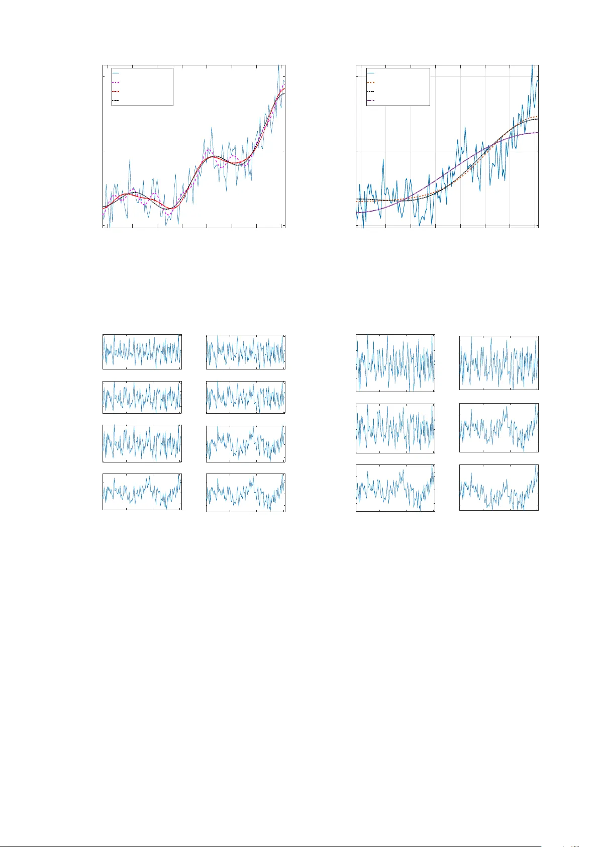
No v el F ourier Quadrature T ransforms and Analytic Signal Represen tations for Nonlinear and Non-stationary Time Series Analysis Pushp endra Singh ∗ ∗ Sc ho ol of Engineering & Applied Sciences, Bennett Univ ersit y – Greater Noida, India Abstract The Hilbert transform (HT) and asso ciated Gabor analytic signal (GAS) represen tation are w ell- kno wn and widely used mathematical form ulations for mo deling and analysis of signals in v arious applications. In this study , like the HT, to obtain quadrature comp onent of a signal, we prop ose the no vel discrete F ourier cosine quadrature transforms (F CQTs) and discrete F ourier sine quadrature transforms (FSQTs), designated as F ourier quadrature transforms (FQTs). Using these F QTs, we prop ose sixteen F ourier-Singh analytic signal (FSAS) representations with follo wing properties: (1) real part of eight FSAS represen tations is the original signal and imaginary part is the F CQT of the real part, (2) imaginary part of eight FSAS representations is the original signal and real part is the FSQT of the real part, (3) like the GAS, F ourier sp ectrum of the all FSAS representations has only p ositive frequencies, ho wev er unlik e the GAS, the real and imaginary parts of the prop osed FSAS representations are not orthogonal to eac h other. The F ourier decomp osition metho d (FDM) is an adaptiv e data analysis approach to decomp ose a signal into a set of small num b er of F ourier in trinsic band functions which are AM-FM comp onen ts. This study also prop oses a new formulation of the FDM using the discrete cosine transform (DCT) with the GAS and FSAS representations, and demonstrate its efficacy for improv ed time-frequency-energy representation and analysis of nonlinear and non-stationary time series. Keywor ds: Hilb ert transform (HT); Gab or analytic signal (GAS) representation; Instan taneous fre- quency (IF); F ourier Quadrature T ransform (F QT); F ourier-Singh analytic signal (FSAS) represen tations; Zero-phase filtering (ZPF) 1 INTR ODUCTION The F ourier theory is the most imp ortan t mathematical to ol for analysis and mo deling physical phenomena and engineering systems. It has b een used to obtain solutions in almost all fields of science and engineering problems. It is the fundamentals of a signal analysis, pro cessing, and interpretation of information. There are man y v arian ts of the F ourier methods suc h as con tinuous time F ourier series (FS) and F ourier transfrom (FT), discrete time F ourier transform (DTFT), discrete time F ourier series (DTFS), discrete F ourier transform (DFT), discrete cosine transform (DCT), and discrete sine transform (DST). All these are orthogonal transforms whic h can b e computed b y the fast F ourier transform (FFT) algorithms. The instantaneous frequency (IF) w as in tro duced by the Carson and F ry [ 1 ] in 1937 with application to the frequency mo dulation (FM), and it w as defined as deriv ativ e of phase of a complex FM signal. Gab or [ 2 ] in 1946 introduced a quadrature metho d based on the F ourier theory as a practical approac h for obtaining the Hilb ert T ransform (HT) of a signal. Ville [ 3 ] in 1948 defined the IF of a real signal b y using Gab or complex extension. Shekel [ 4 ] in 1953 p oin ted out ambiguit y issue in the IF defined by Ville that there are an infinite num b er of pairs of instan taneous amplitude (IA) and IF for a complex extension of a giv en signal. Gab or analytic signal (GAS) represen tation, that has only positive frequencies in the F ourier sp ectrum whic h are identical to that of the real signal, is the fundamental principle of time-frequency analysis. In order to constrain the am biguity issue, V akman [ 5 ] in 1972 had sho wn that the GAS is the only physically-justifiable complex extension for IA and IF estimation, and prop osed the follo wing three conditions to physical realit y: (1) amplitude con tinuit y , (2) phase indep endence of scaling and homogeneity , and (3) harmonic corresp ondence. V akman also sho wed that the HT is the only op erator that satisfies these conditions, th us, the unique complex extension can b e obtained by ∗ Author’s E-mail address: spushp@gmail.com ; pushpendrasingh@iitkalumni.org 1 the GAS representation. Therefore, almost univ ersally , the HT has b een used to construct the GAS represen tation and time-frequency analysis of a nonstationary signal. Several other authors contributed to representation and understanding of IF, Hilb ert sp ectrum analysis, and hav e sho wn that there are problems and paradoxes related to the definition of IF [ 6 – 12 , 39 , 45 ]. In this study , using the DCTs and DSTs which are based on the F ourier theory , we prop ose the F ourier-Singh analytic signal (FSAS) represen tations. The prop osed FSAS satisfies all the ab ov e three conditions of V akman. The DCT w as prop osed in the seminal pap er [ 15 ] with application to image pro cessing for pattern recognition and Wiener filtering. The mo dified DCT (MDCT), prop osed in [ 17 ], is based on the DCT of o verlapping data and uses the concept of time-domain aliasing cancellation [ 18 ]. Due to energy compaction and decorrelation prop erty of the DCT and MDCT, they are extensiv ely used in many audio (e.g. MP3, WMA, AC-3, AA C, V orbis, A TRA C), image (e.g. JPEG) and video (e.g. Motion JPEG, MPEG, Daala, digital video, Theora) compression, electrocardiogram (EEG) data analysis [ 19 ], and for n umerical solution of partial differential equations by sp ectral metho ds. Dep ending up on the b oundary conditions and symmetry ab out a data p oint, there are 8 t yp es of DCTs and 8 t yp es of DSTs. Man y real-life signals such as sp eec h and animal sounds, mec hanical vibrations, seismic wa ve, radar sig- nals, biomedical ECG and electro encephalogram (EEG) signals are nonstationary and generated by non- linear systems. These data can be characterized and mo deled as superp osition of amplitude-mo dulated- frequency-mo dulated (AM-FM) signals. Th us, signal decomp osition, mo de and source separation are imp ortan t for in many applications where receiv ed signal is a sup erp osition of v arious nonstationary signals and noise, and the ob jectiv e is to recov er the original AM-FM constituents. There are many adaptiv e signal decomp osition and analysis metho ds suc h as empirical mo de decomp osition (EMD) algo- rithms [ 10 , 21 – 25 , 29 , 35 ], v ariational mode decomposition (VMD) [ 31 ], sync hrosqueezed wa v elet transforms (SSWT) [ 30 ], eigen v alue decomp osition (EVD) [ 32 ], sparse time-frequency representation (STFR) [ 36 ], empirical wa velet transform (EWT) [ 33 ], resonance-based signal decomp osition (RSD) [ 38 ], and time- v arying vibration decomp osition (TVVD) [ 37 ]. These metho ds are developed based on the p erception whic h has been for man y decades in the literature that F ourier metho d is not suitable for nonlinear and nonstationary data analysis. How ever, the F ourier decomp osition metho d (FDM) proposed in [ 34 , 39 ] is an adaptiv e, nonlinear and nonstationary data analysis metho d based on the F ourier theory and zero-phase filtering (ZPF) approac h. The FDM has demonstrated its efficacy for a nonlinear and nonstationary data analysis in many applications [ 34 , 39 , 42 – 44 ]. In this work, we consider the type-2 DCT [ 15 ], which is the most common v arian t of DCT, to form ulate the FDM. In principle, w e can use any v arian t of DCT or DST to form ulate the FDM. All these metho ds decomp ose the time-domain signal into a set of small num b er of band-limited com- p onen ts and map them into the time-frequency representation (TFR). The TFR pro vides lo calized signal information in b oth time and frequency domain that reveal the complex structure of a signal consisting of sev eral comp onen ts. The IF is the basis of the TFR or time-frequency-energy (TFE) represen tation and analysis of a signal. The IF is a generalization of the definition of the traditional constan t frequency , whic h is required for the analysis of nonstationary signals and nonlinear systems. It is a imp ortant parameter of a signal that can rev eal the underlying pro cess and provides explanations for ph ysical phenomenon in man y applications suc h as atmospheric and meteorological applications [ 10 ], imaging pro cessing for pattern recognition and classification [ 27 , 28 ], mec hanical systems analysis [ 26 ], acoustic, vibration, and sp eec h signal analysis [ 39 ], comm unications, radar, sonar, solar and seismic data analysis [ 39 , 40 ], medical and biomedical applications [ 41 ], time-frequency represen tation of cosmological gra vity w av e [ 47 ]. The main con tributions [ 14 ] of this study are summarized as follo ws: 1. In tro duction of the eigh t discrete F ourier cosine quadrature transform (FCQTs) and eight discrete F ourier sine quadrature transforms (FSQTs) using the eigh t DCTs and eight DSTs, resp ectiv ely . These F CQTs and FSQTs are designated as the F ourier Quadrature T ransforms (FQTs) and thus sixteen FQTs are obtained. 2. In tro duction of the sixteen FSAS representations using sixteen FQTs: (a) eight FSAS represen ta- tions are obtained using the eight DCTs and corresp onding FCQTs, where F ourier sp ectrum of the FSAS has only p ositive frequencies, real part of FSAS is the original signal, imaginary part is the F CQT of the real part, real and imaginary parts are not orthogonal to each other, (b) other eigh t FSAS representations are obtained using the eigh t DSTs and corresp onding FSQTs, where F ourier sp ectrum of the FSAS has only p ositiv e frequencies, imaginary part of FSAS is the original signal, 2 real part is the FSQT of the imaginary part, real and imaginary parts are not orthogonal to eac h other. 3. In tro duction of the t wo contin uous time F QTs, i.e. F CQT and FSQT, using the F ourier cosine trans- form (F CT) and F ourier sine transform (FST), resp ectively . Using these tw o F QTs corresp onding FSAS representations are derived. 4. The new formulations of the FDM are prop osed using DCT and DST with GAS and FSAS repre- sen tations. Th us, in this study , w e present FQTs as effective alternativ es to the HT, and FSAS representations as alternativ es to the GAS represen tation for nonlinear and nonstationary time-series analysis. This study is organized as follo ws: A brief o verview of the analytic signal represen tation and the FDM are presented in Section 2 . FQTs, FSAS representations and new form ulations of the FDM are presented in Section 3 . Sim ulation results and discussions are presen ted in Section 4 . Section 5 presen ts conclusion of the w ork. 2 A brief o v erview of the GAS represen tation, IF and FDM The GAS representation [ 2 ] is a complex-v alued function, z [ n ], that has only p ositiv e frequency comp o- nen ts in the F ourier spectrum, and it is defined as z [ n ] = x [ n ] + j ˆ x [ n ] , (1) where the real part of GAS is the original signal and the imaginary part is the Hilb ert transform (HT) of the real part, real and imaginary part are orthogonal to each other (i.e. inner pro duct h x [ n ] , ˆ x [ n ] i = 0). The HT of a signal is defined as ˆ x [ n ] = H { x [ n ] } = x [ n ] ∗ h [ n ] = ∞ X m = −∞ x [ m ] h [ n − m ] , h [ n ] = 1 − cos( π n ) π n , (2) where ∗ is the con volution op eration, H is Hilb ert op erator and impulse resp onse h [ n ] is the Hilb ert k ernel. F rom ( 2 ), one can observe that the HT is an ideal op erator which cannot be implemen ted in real applications, b ecause, its impulse resp onse is unstable (i.e. absolutely not summable as P ∞ n = −∞ | h [ n ] | = ∞ ), non-causal, and has infinite time support. Practically , the GAS z [ n ], from a real signal x [ n ] of length N , is obtained by the discrete F ourier transform (DFT) as [ 16 , 39 ] z [ n ] = X [0] + N/ 2 − 1 X k =1 2 X [ k ] exp( j 2 π k n/ N ) + X [ N / 2] exp( j π n ) , if N is even , z [ n ] = X [0] + ( N − 1) / 2 X k =1 2 X [ k ] exp( j 2 π k n/ N ) , if N is o dd , (3) where X [ k ] = (1 / N ) P N − 1 n =1 x [ n ] exp( − j 2 π kn/ N ) is the DFT of a signal x [ n ], 0 ≤ n, k ≤ N − 1, exp( j πn ) = ( − 1) n , and X [ N / 2] is the highest frequency component of the F ourier sp ectrum. This is the only practical approac h, based on the F ourier theory and b eing used by MA TLAB as well, which is a v ailable in the literature to obtain the GAS represen tation that satisfies the following prop erties: (P1) only p ositiv e frequencies are present in the F ourier sp ectrum, (P2) real part is the original signal x [ n ], (P3) imaginary part is the HT of real part (i.e. ˆ x [ n ] = H { x [ n ] } ), (P4) real and imaginary parts are orthogonal to eac h other (i.e. h x [ n ] , ˆ x [ n ] i = 0), and (P5) real part is the HT of imaginary part with minus sign (i.e. x [ n ] = − H { ˆ x [ n ] } = − H 2 { x [ n ] } or x [ n ] = H 4 { x [ n ] } ). The GAS ( 1 ) can b e written in p olar representation as z [ n ] = x [ n ] + j ˆ x [ n ] = a [ n ] exp( j φ [ n ]) , (4a) a [ n ] = p x 2 [ n ] + ˆ x 2 [ n ] , (4b) φ [ n ] = arctan( ˆ x [ n ] /x [ n ]) , (4c) f [ n ] = ω [ n ] 2 π = φ d [ n ] 2 π , (4d) 3 where a [ n ], φ [ n ], and f [ n ] are the instan taneous amplitude (IA), instan taneous phase (IP) and the IF, resp ectiv ely . The IF using differentiation of phase in discrete-time, φ d [ n ], can b e approximated by [ 7 ] forw ard finite difference (FFD) or backw ard finite difference (BFD) or central finite difference (CFD) as φ d [ n ] =  φ [ n + 1] − φ [ n ]  , (FFD) (5a) φ d [ n ] =  φ [ n ] − φ [ n − 1]  , (BFD) (5b) φ d [ n ] =  φ [ n + 1] − φ [ n − 1]  / 2 , (CFD) . (5c) The phase in ( 4c ) is computed by the function, atan2( ˆ x [ n ] , x [ n ]), whic h pro duces the result in the range ( − π , π ] and also av oids the problems of division b y zero. It is p ertinent to notice that the IF defined by ( 4d ) is v alid only for mono comp onen t signals b ecause the so-defined IF b ecomes negativ e in some time instan ts for multicomponent signals whic h do es not provide any ph ysical meaning [ 6 , 7 , 10 ]. In order to eliminate this issue and obtain IF p ositive for all the time, b y considering the phase un wrapping fact and multivalue d nature of the inv erse tangent function (i.e. tan( φ [ n ]) = tan( φ [ n ] + k nπ ) , ∀ k , n ∈ Z ), the IF ω [ n ] is defined as [ 13 ] ω [ n ] = ( φ d [ n ] , if φ d [ n ] ≥ 0 , φ d [ n ] + π , otherwise. (6) This definition ( 6 ) makes the IF p ositiv e (i.e. 0 ≤ ω [ n ] ≤ π in radians/sample whic h corresponds to [0 , F s / 2] in Hz) for all time ‘ n ’ which is v alid for all monocomp onent as well as multicomponent signals. The FDM is an adaptiv e signal decomp osition approach which decomp oses a signal, x [ n ], into a set of small n um b er of M analytic F ourier intrinsic band functions (AFIBFs) such that z [ n ] = a 0 + M X i =1 ( x i [ n ] + j ˆ x i [ n ]) = a 0 + M X i =1 a i [ n ] exp( j φ i [ n ]) , (7) where a 0 = X [0] is the a verage v alue of the signal, and x i [ n ] = a i [ n ] cos( φ i [ n ]) , 1 ≤ i ≤ M are amplitude- frequency mo dulated FIBFs which are complete, adaptive, lo cal, orthogonal and uncorrelated b y the virtue of construction [ 39 ]. In the next section, we prop osed a set of analytic signals using DCTs and DSTs whic h satisfy only first tw o prop erties (P1) and (P2). 3 F ourier Quadrature T ransforms, FSAS represen tations and new for- m ulations of the FDM The standard notations for the elemen ts of the DCTs/DSTs transform matrices, C i / S i for i = 1 , 2 , . . . , 8, with their nk -th elemen t, denoted b y ( C i ) nk /( S i ) nk , are defined as [ 20 ] ( C 1 ) nk = aγ n γ k cos  nk π N − 1  , ( C 2 ) nk = bσ k cos  n + 1 2  k π N  , ( C 3 ) nk = bσ n cos  k + 1 2  nπ N  , ( C 4 ) nk = b cos  n + 1 2   k + 1 2  π N  , ( C 5 ) nk = cσ n σ k cos  nk 2 π 2 N − 1  , ( C 6 ) nk = cε n σ k cos  n + 1 2  k 2 π 2 N − 1  , ( C 7 ) nk = cε k σ n cos  k + 1 2  n 2 π 2 N − 1  , ( C 8 ) nk = d cos  n + 1 2   k + 1 2  2 π 2 N + 1  , ( S 1 ) nk = b sin  nk π N  , ( S 2 ) nk = bε k sin  n + 1 2  ( k + 1) π N  , ( S 3 ) nk = bε n sin  k + 1 2  ( n + 1) π N  , ( S 4 ) nk = b sin  n + 1 2   k + 1 2  π N  , ( S 5 ) nk = c sin  nk 2 π 2 N − 1  , ( S 6 ) nk = c sin  n + 1 2   k + 1 2  2 π 2 N − 1  , ( S 7 ) nk = c sin  k + 1 2  ( n + 1)2 π 2 N − 1  , ( S 8 ) nk = cε n ε k sin  n + 1 2   k + 1 2  2 π 2 N − 1  , (8) 4 where constant m ultiplication factors a = q 2 N − 1 , b = q 2 N , c = 2 √ 2 N − 1 , and d = 2 √ 2 N +1 ; normalization factors are unit y except for γ n = 1 √ 2 for n = 0 or N − 1, σ n = 1 √ 2 for n = 0, and ε n = 1 √ 2 for n = N − 1; 0 ≤ n, k ≤ N − 1 for all the N -th-order DCTs/DSTs except for the ( N − 1)-th-order DST-1 and DST-5 where 1 ≤ n, k ≤ N − 1. As the DCTs and DSTs are unitary transform, their in verses are computed b y transp ose relation C − 1 i = C T i and S − 1 i = S T i , resp ectively . Using ( 8 ), w e define the elements of transform matrices as follows ( ˜ S 1 ) nk = aγ n γ k sin  nk π N − 1  , ( ˜ S 2 ) nk = bσ k sin  n + 1 2  k π N  , ( ˜ S 3 ) nk = bσ n sin  k + 1 2  nπ N  , ( ˜ S 4 ) nk = b sin  n + 1 2   k + 1 2  π N  , ( ˜ S 5 ) nk = cσ n σ k sin  nk 2 π 2 N − 1  , ( ˜ S 6 ) nk = cε n σ k sin  n + 1 2  k 2 π 2 N − 1  , ( ˜ S 7 ) nk = cε k σ n sin  k + 1 2  n 2 π 2 N − 1  , ( ˜ S 8 ) nk = d sin  n + 1 2   k + 1 2  2 π 2 N + 1  , ( ˜ C 1 ) nk = b cos  nk π N  , ( ˜ C 2 ) nk = bε k cos  n + 1 2  ( k + 1) π N  , ( ˜ C 3 ) nk = bε n cos  k + 1 2  ( n + 1) π N  , ( ˜ C 4 ) nk = b cos  n + 1 2   k + 1 2  π N  , ( ˜ C 5 ) nk = c cos  nk 2 π 2 N − 1  , ( ˜ C 6 ) nk = c cos  n + 1 2   k + 1 2  2 π 2 N − 1  , ( ˜ C 7 ) nk = c cos  k + 1 2  ( n + 1)2 π 2 N − 1  , ( ˜ C 8 ) nk = cε n ε k cos  n + 1 2   k + 1 2  2 π 2 N − 1  , (9) where seven matrices ˜ S 1 , ˜ S 2 , ˜ S 3 , ˜ S 5 , ˜ S 7 , ˜ C 1 and ˜ C 5 are of ( N − 1)-th-order matrices, and rest other nine matrices are of N -th-order. Using ( 8 ) and ( 9 ), we hereb y define sixteen FQTs (i.e. eight F CQTs, ˜ x c i , and eight F CQTs, ˜ x s i ) and corresp onding sixteen FSAS represen tations (FSASRs), ˜ z c i and ˜ z s i , for i = 1 , 2 , . . . , 8, as follo ws X c i = C i x ; x = C T i X c i ; (DCTs and IDCTs) ˜ x c i = ˜ S T i X c i = ˜ S T i C i x ; ˜ z c i = x + j ˜ x c i ; (F CQTs and FSASRs) X s i = S i x ; x = S T i X s i ; (DSTs and IDSTs) ˜ x s i = ˜ C T i X s i = ˜ C T i S i x ; ˜ z s i = ˜ x s i + j x ; (F CQTs and FSASRs) , (10) where (column v ectors) data x =  x [0] x [1] . . . x [ N − 1]  T ; X c i =  X c i [0] X c i [1] . . . X c i [ N − 1]  T and X s i =  X s i [0] X s i [1] . . . X s i [ N − 1]  T are the DCT and DST of i -th t yp e, resp ectiv ely . Thus, we ha ve defined linear transformations of x in to ˜ x c i , and x in to ˜ x s i with orthogonal transformation matrices ˜ S T i C i and ˜ C T i S i , resp ectively . These transformation matrices are orthogonal due to the prop erties of an orthogonal matrix (i.e., if Q is an orthogonal matrix, then so is Q T and Q T = Q − 1 ; if Q 1 and Q 2 are orthogonal matrices, then so is Q 1 Q 2 ). The contin uous time FCQT, FSQT and corresp onding FSAS representations are defined in Appendix A . The prop osed 2D FSAS representations are defined in App endix B . No w, we consider the complete process of obtaining F QT, corresponding FSAS and FDM using DCT-2 as follows. The DCT-2 of a sequence, x [ n ] of length N , is defines as [ 15 ] X c2 [ k ] = r 2 N σ k N − 1 X n =0 x [ n ] cos  π k (2 n + 1) 2 N  , 0 ≤ k ≤ N − 1 , (11) and inv erse DCT (IDCT) is obtained by x [ n ] = r 2 N N − 1 X k =0 σ k X c2 [ k ] cos  π k (2 n + 1) 2 N  , 0 ≤ n ≤ N − 1 , (12) 5 where normalization factors σ k = 1 √ 2 for k = 0, and σ k = 1 for k 6 = 0. If consecutive samples of sequence x [ n ] are correlated, then DCT concentrates energy in a few X c2 [ k ] and decorrelates them. The DCT basis sequences, cos  π k (2 n +1) 2 N  , which are a class of discrete Chebyshev polynomials [ 15 ], form an orthogonal set as inner pro duct D cos  π k (2 n +1) 2 N  , cos  π m (2 n +1) 2 N E = 0 for k 6 = m , and N − 1 X n =0 cos  π k (2 n + 1) 2 N  cos  π m (2 n + 1) 2 N  =      N , k = m = 0 , N / 2 , k = m 6 = 0 , 0 , k 6 = m. (13) W e hereby formally define the discrete F ourier cosine quadrature transform (FCQT), ˜ x c2 [ n ], of a signal x [ n ] as ˜ x c2 [ n ] = r 2 N N − 1 X k =0 X c2 [ k ] sin  π k (2 n + 1) 2 N  , 0 ≤ n ≤ N − 1 , (14) where X c2 [ k ] is the DCT-2 of a signal x [ n ]. Since, for frequency k = 0, in ( 14 ), basis v ector sin  π k (2 n +1) 2 N  is zero, so w e can write F CQT as ˜ x c2 [ n ] = q 2 N P N − 1 k =1 X c2 [ k ] sin  π k (2 n +1) 2 N  and obtain ˜ X c2 [ k ] from ( 14 ) as ˜ X c2 [ k ] = r 2 N N − 1 X n =0 ˜ x c2 [ n ] sin  π k (2 n + 1) 2 N  , 0 ≤ k ≤ N − 1 , (15) where ˜ X c2 [ k ] = ( 0 , k = 0 , X c2 [ k ] , 1 ≤ k ≤ N − 1 . (16) One can observe that X c2 [ k ] defined in ( 11 ) and ˜ X c2 [ k ] ( 15 ) are exactly same for zero-mean signal (i.e. X c2 [0] = 0), otherwise, they are different only for k = 0. The IDCT of ˜ X c2 [ k ] is original signal less DC comp onen t. The proposed FCQT ( 14 ) uses the basis sequences, sin  π k (2 n +1) 2 N  , whose inner pro duct is defined as N − 1 X n =0 sin  π k (2 n + 1) 2 N  sin  π m (2 n + 1) 2 N  =      0 , k = m = 0 , N / 2 , k = m 6 = 0 , 0 , k 6 = m, (17) and, therefore, the set of these basis v ectors form an orthogonal set for 1 ≤ k ≤ N − 1. F rom ( 11 ) and ( 14 ), one can easily observe that the FCQT of a constan t signal, lik e the HT, is zero. The vector space theoretic approac h and explanation of this prop osed transformation is as follows. Let V and W b e vector spaces, a function T : V → W is called a linear transformation if for an y vectors v 1 , v 2 ∈ V and scalar c , (1) T ( v 1 + v 2 ) = T ( v 1 ) + T ( v 2 ), and (2) T ( c v 1 ) = cT ( v 1 ). Here in this study , V is a vector space spanned by the set of cosine basis vectors, n cos  π k (2 n +1) 2 N o for 0 ≤ k ≤ N − 1, with dimension N , and W is a v ector space spanned by the set of sine basis v ectors, n sin  π k (2 n +1) 2 N o for 0 ≤ k ≤ N − 1, with dimension ( N − 1). Therefore, these tw o vector spaces are homomorphic, transformation is linear and non-inv ertible as a constant v ector is mapp ed to the zero v ector. How ev er, for a zero mean vector x [ n ] (i.e. X c2 [0] = 0), these tw o vector spaces are isomorphic, transformation is linear and in vertible, and a set of orthogonal cosine basis vectors are mapped to the set of orthogonal sine basis vectors, i.e., n cos  π k (2 n +1) 2 N o 7→ n sin  π k (2 n +1) 2 N o or T  cos  π k (2 n +1) 2 N  =  sin  π k (2 n +1) 2 N  for 1 ≤ k ≤ N − 1. Th us, the linear transformation of x [ n ] into ˜ x c2 [ n ], defined in ( 10 ) and ( 14 ) with transformation matrix ˜ S T 2 C 2 , is (a) non-inv ertible if the mean of signal x [ n ] is non-zero, and (b) inv ertible if the mean of signal x [ n ] is zero. In practice, we can alwa ys remov e the mean from x [ n ] to mak e it a zero mean vector, that leads the prop osed transformation to be isomorphic. Using 8 t yp es of DCTs and 8 types of DSTs, w e prop ose to obtain 16 different types of FSAS rep- resen tations as presented in ( 10 ). In this study , w e esp ecially consider DCT-2 to obtain the FSAS as ˜ z c2 [ n ] = r 2 N N − 1 X k =0 σ k X c2 [ k ] exp  j π k (2 n + 1) 2 N  = x [ n ] + j ˜ x c2 [ n ] , 0 ≤ n ≤ N − 1 , (18) 6 where j = √ − 1, real part of ˜ z c2 [ n ] is the original signal, and imaginary part of ˜ z c2 [ n ] is the FQT of real part. It is w orthwhile to note that the signal x [ n ] and its FQT ˜ x c2 [ n ] are not orthogonal, i.e. h x [ n ] , ˜ x c2 [ n ] i 6 = 0. T o prov e this, we consider the inner pro duct of basis sequences, cos  π k (2 n +1) 2 N  and sin  π m (2 n +1) 2 N  , and using trigonometric manipulation [2 cos( α ) sin( β ) = sin( α + β ) − sin( α − β ), sin(2 α ) = 2 sin( α ) cos( α ), 2 sin 2 ( α ) = 1 − cos(2 α )] show that it is not zero for some k 6 = m , i.e. N − 1 X n =0 cos  π k (2 n + 1) 2 N  sin  π m (2 n + 1) 2 N  =            0 , k = m = 0 , 0 , k = m 6 = 0 , 0 , k 6 = m, and m ± k = 2 l , Σ m,k = Σ m + k + Σ m − k , k 6 = m, and m ± k = (2 p + 1) , (19) where Σ m ± k = 1 2 P N − 1 n =0 sin  π (2 n +1)( m ± k ) 2 N  , 0 ≤ l ≤ ( N − 1), and 0 ≤ p ≤ ( N − 2). W e obtain sum of exp onen tial series as, E m ± k = h P N − 1 n =0 exp  j π (2 n +1)( m ± k ) 2 N i = " exp  j π ( m ± k ) 2  sin  π ( m ± k ) 2  sin  π ( m ± k ) 2 N  # , which implies E m ± k = " sin( π ( m ± k )) 2 sin  π ( m ± k ) 2 N  + j [1 − cos( π ( m ± k ))] 2 sin  π ( m ± k ) 2 N  # . Thus, real part Re { E m ± k } = 0 if m 6 = k ; imaginary part Im { E m ± k } = 0 if m ± k = 2 l , and Im { E m ± k } = 1 sin  π ( m ± k ) 2 N  if m ± k = 2 p + 1, Σ m ± k = 1 2 Im { E m ± k } , and | Σ m,k | → ∞ when N → ∞ with m ± k = 2 p + 1. No w, w e propose the DCT based FDM (i.e. DCT-FDM), and devise t wo new approac hes to decomp ose a signal in to a small set of AM-FM signals (i.e. FIBFs) and corresp onding analytic represen tations. In the first approach, w e obtain the decomp osition of signal x [ n ] (excluding the DC comp onen t) into a set of FIBFs, { x i [ n ] } M i =1 , and corresponding AFIBFs, { ˜ z c2 i [ n ] } M i =1 , using the FSAS representation ( 18 ) as ˜ z c2 [ n ] = r 2 N N − 1 X k =1 X c2 [ k ] exp  j π k (2 n + 1) 2 N  = M X i =1 ˜ z c2 i [ n ] , 0 ≤ n ≤ N − 1 , (20) where ˜ z c21 [ n ] = q 2 N P N 1 k =1 X c2 [ k ] exp  j π k (2 n +1) 2 N  , ˜ z c22 [ n ] = q 2 N P N 2 k = N 1 +1 X c2 [ k ] exp  j π k (2 n +1) 2 N  , . . . , ˜ z c2 M [ n ] = q 2 N P N M k = N M − 1 +1 X c2 [ k ] exp  j π k (2 n +1) 2 N  , which can b e written as ˜ z c2 i [ n ] = r 2 N N i X k = N i − 1 +1 X c2 [ k ] exp  j π k (2 n + 1) 2 N  = x i [ n ] + j ˜ x c2 i [ n ] , 1 ≤ i ≤ M , (21) where N 0 = 0 and N M = N − 1. In the second approach, using the DCT-FDM, we decomp ose the signal x [ n ] in to the same set of FIBFs, { x i [ n ] } M i =1 , and apply the Hilb ert transform to obtain corresp onding set of AFIBFs, { ˆ z i [ n ] } M i =1 , using the GAS represen tation as ˆ z [ n ] = M X i =1 ˆ z i [ n ] , ˆ z i [ n ] = x i [ n ] + j ˆ x i [ n ] , 1 ≤ i ≤ M , (22) where ˆ x i [ n ] is the HT of x [ n ], h x i [ n ] , ˆ x i [ n ] i = 0, and x i [ n ] = r 2 N N i X k = N i − 1 +1 X c2 [ k ] cos  π k (2 n + 1) 2 N  . (23) It is pertinent to note that in the FDM ( 22 ) all five prop erties (P1)–(P5) of the GAS are satisfied, ho w ever, in the FDM ( 21 ), whic h uses FSAS, only first t w o prop erties (P1) and (P2) of the GAS are being satisfied. The blo ck diagrams of the FDM, using DCT based zero-phase filter-bank to decompose a signal in to a set of desired frequency bands, are shown in Figure 1 , where, for each i ∈ [1 , M ], H i [ k ] = ( 1 , ( N i − 1 + 1) ≤ k ≤ N i , 0 , otherwise. (24) 7 x [ n ] DCT . . . H 1 [ k ] H 2 [ k ] H M [ k ] FSAS FSAS . . . FSAS ˜ z c21 [ n ] ˜ z c22 [ n ] . . . ˜ z c2 M [ n ] x [ n ] DCT . . . H 1 [ k ] H 2 [ k ] H M [ k ] IDCT IDCT . . . IDCT GAS GAS . . . GAS ˆ z 1 [ n ] ˆ z 2 [ n ] . . . ˆ z M [ n ] Figure 1: Blo ck diagrams of the FDM using DCT based zero-phase filter-bank to decomp ose a signal x [ n ] in to the set of orthogonal desired frequency bands (a) { ˜ z c21 [ n ] , ˜ z c22 [ n ] , · · · , ˜ z c2 M [ n ] } using ( 20 ) and ( 21 ); (b) { ˆ z 1 [ n ] , ˆ z 2 [ n ] , · · · , ˆ z M [ n ] } using ( 22 ) and ( 23 ). W e hav e used ZPF where frequency resp onse of filter is one in the desired band and zero otherwise. Moreo ver, one can use any other kind of ZPF (i.e. H i [ k ] ∈ R ≥ 0 , ∀ i, k ) such as the Gaussian filter to decomp ose a signal. The FDM advocates to use ZPF b ecause it preserves salient features such as minima and maxima in the filtered w av eform exactly at the p osition where those features o ccur in the original unfiltered wa v eform. Based on the requiremen t and t yp e of application, we can devise metho ds to select ranges of frequency parameter k in ( 24 ), e.g., one can use three approac hes to divide complete frequency band of a signal under analysis in to small n umber of equal, dyadic, and equal-energy frequency bands. T o obtain TFE represen tation of a signal using ( 20 ) and ( 22 ), w e write FSAS and GAS in p olar represen tation, for 1 ≤ i ≤ M , as ˜ z c2 i [ n ] = ˜ a i [ n ] e j ˜ φ i [ n ] , ˜ φ i [ n ] = tan − 1 ( ˜ x c2 i [ n ] /x i [ n ]) , ˜ ω i [ n ] = ˜ φ id [ n ] , (25a) ˆ z i [ n ] = ˆ a i [ n ] e j ˆ φ i [ n ] , ˆ φ i [ n ] = tan − 1 ( ˆ x i [ n ] /x i [ n ]) , ˆ ω i [ n ] = ˆ φ id [ n ] , (25b) where IA ( ˜ a i [ n ], ˆ a i [ n ]) and IF ( ˜ ω i [ n ], ˆ ω i [ n ]) are computed by ( 4b ) and ( 4d ), respectively . Finally , using the prop osed FSAS and the GAS represen tations, the three dimensional TFE distributions are obtained b y plotting { n, ˜ f i [ n ] , ˜ a 2 i [ n ] } and { n, ˆ f i [ n ] , ˆ a 2 i [ n ] } , resp ectively . 4 Results and discussions In this section, to demonstrate the efficacy of the prop osed metho ds—DCT and FSAS based FDM (DCT- FSAS-FDM), DCT and GAS based FDM (DCT-GAS-FDM)—we consider many sim ulated as well as real-life data, and compare the obtained results with other p opular metho ds suc h EMD, CWT, DFT and GAS based FDM (DFT-GAS-FDM), FIR and GAS based FDM (FIR-GAS-FDM). W e mainly consider those signals whic h hav e b een widely used in literature for p erformance ev aluation and results comparison among prop osed and other existing metho ds. 4.1 A unit sample sequence analysis First, we consider an analysis of unit sample (or unit impulse or delta) sequence using the prop osed FSAS and compare the results with GAS representation. A unit sample function is defined as δ [ n − n 0 ] = 1 for n = n 0 , and δ [ n − n 0 ] = 0 for n 6 = n 0 . Using the inv erse F ourier transform, analytic representation, z [ n ] = 1 π R π 0 X ( ω ) exp( j ω n ) d ω , of a signal x [ n ] = δ [ n − n 0 ] ⇔ X ( ω ) = exp( − j ωn 0 ) is obtained as [ 39 ], z [ n ] = sin( π ( n − n 0 ))+ j [1 − cos( π ( n − n 0 ))] π ( n − n 0 ) = a [ n ] exp( j φ [ n ]), where real part of z [ n ] is δ [ n − n 0 ] = sin( π ( n − n 0 )) π ( n − n 0 ) , a [ n ] = | sin( π 2 ( n − n 0 )) π 2 ( n − n 0 )) | (IA), φ [ n ] = π 2 ( n − n 0 ) (IP), and therefore ω [ n ] = π 2 (IF) whic h corresp onds to half of the Nyquist frequency , that is, F s 4 Hz. Theoretically , this representation demonstrates that most of the energy of signal, δ [ n − n 0 ], is concen trated at time, t = 4 . 99 s ( n 0 = 499) and frequency f = 25 Hz, where sampling frequency , F s = 100 Hz, and length of signal, N = 1000, are considered. The plots of IA, IF and TFE using the GAS and FSAS representations are sho wn in Figure 2 (a) and 2 (b), resp ectiv ely . In the GAS representation, Figure 2 (a), IF is v arying b etw een 0 to 50 Hz at both ends of signal and conv erges to theoretical v alue only at the p osition of delta function. On the other hand, the FSAS represen tation yields b etter results as it pro duces correct v alue of IF, Figure 2 (b), for all the time. 8 (a) 0 1 2 3 4 5 6 7 8 9 Time (s) 0 0.5 1 a[n] 0 1 2 3 4 5 6 7 8 9 Time (s) 0 25 50 Frequency (Hz) 0 50 0.5 9 a[n] 8 Frequency (Hz) Time (s) 7 25 6 5 1 4 3 2 1 0 0 (b) 0 1 2 3 4 5 6 7 8 9 Time (s) 0 0.5 1 a[n] 0 1 2 3 4 5 6 7 8 9 Time (s) 0 25 50 Frequency (Hz) 0 50 0.5 9 a[n] 8 Frequency (Hz) 7 25 6 Time (s) 5 1 4 3 2 1 0 0 Figure 2: Analysis of unit sample sequence: time-amplitude (top), time-frequency (middle) and time- frequency-amplitude (b ottom) subplots (a) and (b) obtained using the GAS and FSAS representations, resp ectiv ely . 4.2 Chirp signal analysis In this example, we consider an analysis of a non-stationary c hirp signal using the prop osed FSAS and compare the results with GAS approach, with sampling frequency F s = 1000 Hz, time duration t ∈ [0 , 1) s and frequency f ∈ [5 , 100) Hz. Figure 3 (a) shows chirp signal (5Hz–100Hz) (top), prop osed FCQT (middle) obtained using ( 14 ) whic h is also imaginary part of the prop osed FSAS ( 18 ), and HT (b ottom) that is imaginary part of the GAS represen tation ( 3 ), which has unnecessary distortions at b oth ends of the signal. The TFE distributions obtained (1) using the FSAS representation is sho wn in Figure 3 (b), and (2) using the GAS represen tation is shown in Figure 3 (c), whic h has lot of energy spreading o ver wide range of time-frequency plane, at b oth ends of the signal under analysis. These examples, 4.1 and 4.2 , clearly demonstrate the adv an tage of the prop osed FSAS o ver the GAS representation for TFE analysis of a signal. 4.3 Sp eec h signal analysis An estimation of the instan taneous fundamen tal frequency F 0 is a most imp ortant problem in sp eec h pro cessing, b ecause it arises in numerous applications, such as language iden tification [ 50 ], sp eak er recog- nition [ 51 ], emotion analysis [ 52 ], sp eec h compression and v oice con version [ 53 , 54 ]. Figure 4 (a) sho ws a segmen t of v oiced sp eec h signal (top) from CMU-Arctic database [ 49 ] sampled at F s = 32000 Hz, corre- sp onding electroglottograph (EGG) signal (middle), and differenced EGG (b ottom) signal. Figure 4 (b), top plot, sho ws magnitude spectrum of sp eec h signal where F 0 is around 132 Hz, and energy of sp eech signal is concen trated on harmonics of F 0 , and the magnitude sp ectrum of differenced EGG (DEGG) sig- nal is sho wn in b ottom plot that also indicate F 0 around 132 Hz. Figure 4 (c) sho ws a decomp osition of sp eec h segment in to a set of nine FIBFs (FIBF1–FIBF9) and a low frequency component (LF C) using the FDM. Figure 4 (d) presen ts TFE representation obtained from the FDM where F 0 and its harmonics are clearly separated in distinct frequency bands. Th us, the FDM is able to ac hiev e and follo w the proposed mo del ( 7 ) precise ly . 4.4 Noise remo v al from ECG signal Electro cardiogram (ECG) signals, records of the electrical activit y of the heart, are used to examine the activit y of human heart. There are v arious problems that may arise while recording an ECG signal. It ma y b e distorted due to the presence of v arious noises suc h as channel noise, baseline w ander (BL W) noise (of generally b elow 0.5 Hz), p o wer-line in terference (PLI) of 50 Hz (or 60 Hz), and ph ysiological artifact. Due to these noises, it b ecomes difficult to diagnose diseases, and th us appropriate treatment ma y b e impacted [ 55 ]. The BL W and PLI remov al from an ECG signal (obtained from MIT-Arrhythmia 9 (a) -1 0 1 Chirp signal -2 0 2 Imaginary part of FSAS 0 0.1 0.2 0.3 0.4 0.5 0.6 0.7 0.8 0.9 1 -2 0 2 Imaginary part of GAS (b) Time-Frequency-Energy plot 0 0.1 0.2 0.3 0.4 0.5 0.6 0.7 0.8 0.9 Time (s) 20 40 60 80 100 120 140 Frequency (Hz) (c) Time-Frequency-Energy plot 0 0.1 0.2 0.3 0.4 0.5 0.6 0.7 0.8 0.9 Time (s) 20 40 60 80 100 120 140 Frequency (Hz) Figure 3: Analysis of a non-stationary signal: (a) A c hirp signal (5Hz–100Hz) (top), F CQT–imaginary part of the prop osed FSAS (middle), HT–imaginary part of GAS (b ottom); obtained TFE represen tations using the FSAS (b), and GAS (c). database, F s = 360 Hz) using the prop osed metho d is sho wn in Figure 5 : (a) a segment of clean ECG signal (top), ECG signal hea vily corrupted (i.e., SNR is lo w, in the range ≈ − 18 . 4 dB) with BL W and PLI (b ottom) noises, (b) ECG signal after noise remo v al (top), separated BL W (middle) and PLI (b ottom). Th us, prop osed FDM can b e used to remo ve BL W and PLI noises, and recov er ECG signal ev en in scenarios where signal-to-noise ratio (SNR) is rather p o or. 4.5 T rend and v ariability estimation from a nonlinear and nonstationary time series Estimating trend and p erforming detrending op erations are important steps in numerous applications, e.g., in climatic data analyses, the trend is one of the most critical parameters [ 57 ]; in sp ectral analysis and in estimating the correlation function, it is necessary to remo ve the trend from the data to obtain meaningful results [ 57 ]. Thus, in signal and other data analysis, it is crucial to estimate the trend, detrend the data, and obtain v ariabilit y of the time series at any desired time scales. The Global surface temp erature anomaly (GST A) data (of 148 Y ears from 1856 to 2003, publicly a v ailable at [ 56 ]) analysis and its trend obtained from the prop osed metho d is shown in Figure 6 : (a) GST A data (blue solid), and its trend (red dashed, sixty four-y ears or longer time scale) obtained by dividing data in to six dyadic frequency bands, and corresp onding FIBFs (b). Figure 6 (c) obtained by decomp osing the data in to tw elv e FIBFs of non-dyadic frequency bands: FIBF11 shows (2–3) y ears time scale v ariations, FIBF10 (3–4), FIBF9 (4–6), FIBF8 (6–8), FIBF7 (8–12), FIBF6 (12–16), FIBF5 (16–24), FIBF4 (24–32), FIBF3 (32–44), FIBF2, (44–64), FIBF1 (64–80 years), and trend sho ws 80 years or longer 10 (a) 0 0.05 0.1 0.15 0.2 0.25 -0.4 -0.2 0 0.2 0.4 Amplidude 0 0.05 0.1 0.15 0.2 0.25 -0.5 0 0.5 Amplidude 0 0.05 0.1 0.15 0.2 0.25 Time (s) -0.1 -0.05 0 Amplidude (b) 500 1000 1500 2000 2500 3000 3500 4000 4500 5000 f (Hz) 0.01 0.02 0.03 0.04 0.05 Speech Spectrum 0 500 1000 1500 2000 2500 3000 3500 4000 4500 5000 f (Hz) 0.5 1 1.5 2 2.5 DEGG Spectrum 10 -3 (c) -0.05 0 0.05 0.1 FIBF11 -0.01 0 0.01 FIBF10 -0.05 0 0.05 FIBF9 -0.05 0 0.05 FIBF8 -0.1 0 0.1 FIBF7 -0.05 0 0.05 FIBF6 -0.2 0 0.2 FIBF5 -0.1 0 0.1 FIBF4 -0.04 -0.02 0 0.02 0.04 FIBF3 -0.05 0 0.05 FIBF2 0 0.05 0.1 0.15 0.2 0.25 -0.05 0 0.05 FIBF1 0 0.05 0.1 0.15 0.2 0.25 -4 -2 0 2 LFC 10 -3 (d) Time-Frequency-Energy plot 0 0.05 0.1 0.15 0.2 0.25 Time (s) 0 500 1000 1500 2000 2500 3000 3500 4000 Frequency (Hz) Figure 4: Analysis of sp eech signal: (a) A segmen t of speech (top), EEG (middle) and DEGG (b ottom) signals, (b) Spectrum fo sp eech (top) and DEGG (b ottom) signals, (c) Set of FIBFs obtained by the prop osed DCT based FDM, and (d) TFE representation b y prop osed method. time scale v ariations of temp erature. T o demonstrate the efficacy of the prop osed FDM to estimate a trend and v ariability from data at an y desired time scale, e.g., we estimated the trends and v ariabilities of GST A data in v arious time scales as shown in Figure 6 (d), Figure 7 and Figure 8 . Figure 6 (d) shows GST A data (blue solid), and trends (red dashed) in multiple of 10 (i.e. 10–80) years or longer time scale v ariations of temp erature. Figure 7 presen ts: (a) GST A data, and its trend in 15, 25 and 53 years or longer time scale, and (b) GST A data, and its trend in 75, 100 and 125 y ears or longer time scale. The v ariabilities of the annual GST A data corresp onding to v arious trends (i.e. data min us corre- sp onding trends) with their time scales are giv en in Figure 8 : (a) v ariabilities corresp onding to trends in Figure 6 (d), and (b) v ariabilities corresp onding to trends in Figure 7 . F rom these Figures, it is clear that the v ariabilities up to 53 years or longer time scale are similar and don’t con tain any low frequency comp onen t (i.e. there is no mo de-mixing). How ever, the v ariabilities from 60 years (in fact exp erimen- tally found 54 y ears Figure 9 ) or longer time scale are different from up to 53 y ears and also con tain lo w frequency comp onent (i.e. there is mo de-mixing). The trend and v ariability analysis of this climate data is also p erformed b y the EMD algorithm in [ 57 ]. The EMD algorithm decomp oses the climate data in to a set of IMFs which ha ve o v erlapping frequency sp ectra and their cutoff frequencies are also not under con trol, therefore, the trend and v ariabilit y of data at desired time scales with clear demarcation cannot b e obtained. F or example, we hav e shown that there is a significant change in the trend and v ariabilit y of data in just one year difference of time scale 11 (a) 0 2 4 6 8 10 12 14 16 18 20 -100 0 100 200 300 0 2 4 6 8 10 12 14 16 18 20 Time (s) -1000 -500 0 500 1000 (b) 0 2 4 6 8 10 12 14 16 18 20 -500 0 500 0 2 4 6 8 10 12 14 16 18 20 -1000 0 1000 0 2 4 6 8 10 12 14 16 18 20 Time (s) -500 0 500 Figure 5: Noise remo v al from ECG signal using the prop osed metho d: (a) A segment of clean ECG signal (top), ECG signal corrupted (SNR ≈ − 18 . 4 dB) with baseline wander and p o wer-line in terference (b ottom), (b) ECG signal after noise remov al (top), estimated baseline wander (middle) and p o wer-line in terference (bottom). (observ e change in 53 y ears or longer time scale to 54 years or longer time scale in Figure 9 ). This kind of fine control along with determination of trend and v ariabilit y of data in desired time scale with clear demarcation can b e obtained by the proposed metho d, whic h is not ac hiev able b y the EMD and its related algorithms. 4.6 Seismic signal analysis An Earthquake time series is nonlinear and nonstationary in nature and in this example we consider the Elcen tro Earthquak e data. The Elcen tro Earthquak e time series (which is sampled at F s = 50 Hz) has b een do wnloaded from [ 46 ] and is sho wn in top Figure 10 (a). The most critical frequency range that matters in the structural design is less than 10 Hz, and the F ourier p ow er spectral density (PSD), b ottom Figure 10 (a), sho ws that almost all the energy in this Earthquake time series is present within 10 Hz. Figure 10 presen ts: (b) TFE distributions b y the DCT based FDM metho d without decomp osition, (c) FIBFs obtained b y decomp osing data into eight dyadic bands [FIBF0 (0–0.1953), FIBF1 (0.1953–0.390), FIBF2 (0.390–0.78125), FIBF3 (0.78125–1.5625), FIBF4 (1.5625–3.125), FIBF5 (3.125–6.25), FIBF6 (6.25–12.5), FIBF7 (12.5–25)] Hz, (d) ten equal energy FIBFs [FIBF0 (0–927.7344e-003), FIBF0 (927.7344e-003– 1.1841), FIBF2 (1.1841–1.5015), FIBF3 (1.5015–1.8433), FIBF4 (1.8433–2.1606), FIBF5 (2.1606–2.6733), FIBF6 (2.6733–3.7109), FIBF7 (3.7109–4.7119), FIBF8 (4.7119–6.8237), FIBF9 (6.8237–25)] Hz, (e) TFE distribution corresp onding eigh t dy adic bands, and (f ) TFE distribution corresp onding ten equal energy bands. The obtained TFE distributions indicate that the maximum energy in the signal is presen t around 2 second and 1.7 Hz. These FIBFs and TFE distributions pro vide details of ho w the differen t wa v es arrive from the epical cen ter to the recording station, for example, the compression wa v es of small amplitude and higher frequency range 12 to 25 Hz [e.g. FIBF7 of Figure 10 (c)], the shear and surface w av es of strongest amplitude and low er frequency range of b elo w 12 Hz [e.g. FIBF6, FIBF5, FIBF4 and FIBF3 of Figure 10 (c)] whic h create most of the damage in structure, and other b o dy shear wa v es of low est amplitude and frequency range of b elow 1 Hz [e.g. FIBF2, FIBF1, and FIBF0 of Figure 10 (c)] which are presen t o v er the full duration of the time series. 4.7 Gra vitational wa v e ev en t GW150914 analysis: Noise remov al, IF and TFE esti- mation Gra vitational wa v es (GWs), predicted in 1916 by Alb ert Einstein, are ripples in the space-time con tin uum that tra vel outw ard from a source at the speed of light, and carry with them information ab out their source of origin. The GW ev ent GW150914, pro duced b y a binary blac k hole merger nearly 1.3 billion light y ears a wa y [ 47 ], marks one of the greatest scien tific disco veries in the history of human life. In this example, 12 (a) 1860 1880 1900 1920 1940 1960 1980 2000 Year -0.6 -0.4 -0.2 0 0.2 0.4 0.6 Kelvin The annual mean global surface temperature anomaly data Sixty four-years or longer time scale trend using proposed FDM (b) -0.1 0 0.1 FIBF5 -0.1 0 0.1 FIBF4 -0.05 0 0.05 0.1 FIBF3 -0.05 0 0.05 FIBF2 1900 1950 2000 -0.1 0 0.1 FIBF1 1900 1950 2000 -0.2 0 0.2 FIBF0 (c) -0.05 0 0.05 0.1 FIBF11 -0.05 0 0.05 FIBF10 -0.05 0 0.05 FIBF9 -0.05 0 0.05 FIBF8 -0.05 0 0.05 FIBF7 -0.02 0 0.02 FIBF6 -0.05 0 0.05 FIBF5 -0.02 0 0.02 FIBF4 -5 0 5 FIBF3 10 -3 -0.1 0 0.1 FIBF2 1900 1950 2000 -0.05 0 0.05 FIBF1 1900 1950 2000 -0.2 0 0.2 Trend (d) -0.5 0 0.5 10-years or longer time scale trend -0.5 0 0.5 20-years or longer time scale trend -0.5 0 0.5 30-years or longer time scale trend -0.5 0 0.5 40-years or longer time scale trend -0.5 0 0.5 50-years or longer time scale trend -0.5 0 0.5 60-years or longer time scale trend 1900 1950 2000 -0.5 0 0.5 70-years or longer time scale trend 1900 1950 2000 -0.5 0 0.5 80-years or longer time scale trend Figure 6: The GST A data analysis using the proposed FDM: (a) GST A data (blue solid), and its trend (red dashed) obtained by dividing data in to six dyadic frequency bands, and corresp onding dyadic FIBFs (b), (c) FIBFs obtained by dividing data into tw elve non-dyadic frequency bands, and (d) GST A data (blue solid) and trends (red dashed) in v arious time scales of 10–80 years or longer. using the prop osed metho d, we consider the noise remov al, IF estimation and TFE represen tation of this GW even t data whic h is publicly av ailable at [ 48 ] (sampling rate F s = 16384 Hz). The GW signal sw eeps upw ards in frequency from 35 Hz to 250 Hz, and amplitude strain increases to a peak GW strain of 1 . 0 × 10 − 21 [ 47 ]. The noise remov al and an accurate IF estimation of the GW data is important b ecause IF is the basis to estimate man y parameters such as v elo city , separation, luminosit y distance, primary mass, secondary mass, c hirp mass, total mass, and effective spin of binary blac k hole merger [ 47 ]. Figure 11 shows (a) the GW H1 strain data GW150914 (top figure) observ ed at the laser in terferometer gra vitational-w av e observ atory (LIGO) Hanford whic h is hea vily corrupted with noise, the F ourier sp ectrum (b ottom figure) of the GW data which is not able to capture the non-stationarit y (i.e. up wards sw eep in the frequency and amplitude) present in the data, (b) the TFE representation of the GW H1 data b y prop osed metho d whic h shows the signal frequency is increasing with time but ha ving lots of unnecessary fluctuations in frequency due to noise, and (c) decomp osition of data into a set of six FIBFs [FIBF1 (25–60), FIBF2 (60– 100), FIBF3 (100–200), FIBF4 (200–300), FIBF5 (300–350), FIBF6 (350–8192)] Hz and a lo w frequency comp onen t (LF C) 0–25 Hz), (d) FW1-FW5 are obtained b y m ultiplying the time domain Gaussian window with corresp onding FIBFs (FIBF1-FIBF5), and the reconstructed GW (RGW) is obtained by summation of FW1-FW5 comp onents. In the reconstruction of wa v e, the LF C and FIBF6 ha ve b een ignored as they are out of band noises presen t in the GW H1 data. The further analysis, comparison, residue and TFE estimation of GW even t GW150914 H1 strain data 13 (a) 1860 1880 1900 1920 1940 1960 1980 2000 -0.5 0 0.5 The annual mean global surface temperature anomaly GSTA data 15 years or longer time scale trend 25 years or longer time scale trend 53 years or longer time scale trend (b) 1860 1880 1900 1920 1940 1960 1980 2000 Year -0.5 0 0.5 Kelvin The annual mean global surface temperature anomaly GSTA data 75 years or longer time scale trend 100 years or longer time scale trend 125 years or longer time scale trend Figure 7: T rend analysis of GST A data using the prop osed FDM: (a) GST A data, and its trend in 15, 25 and 53 years or longer time scale, (b) GST A data, and its trend in 75, 100 and 125 years or longer time scale. (a) -0.2 0 0.2 10-years or longer time scale variability -0.1 0 0.1 0.2 20-years or longer time scale variability -0.1 0 0.1 0.2 30-years or longer time scale variability -0.2 0 0.2 40-years or longer time scale variability -0.2 0 0.2 50-years or longer time scale variability -0.2 0 0.2 60-years or longer time scale variability 1900 1950 2000 -0.2 0 0.2 70-years or longer time scale variability 1900 1950 2000 -0.2 0 0.2 80-years or longer time scale variability (b) -0.1 0 0.1 0.2 15-years or longer time scale variability -0.1 0 0.1 0.2 25-years or longer time scale variability -0.2 0 0.2 53-years or longer time scale variability -0.2 0 0.2 75-years or longer time scale variability 1900 1950 2000 -0.2 0 0.2 100-years or longer time scale variability 1900 1950 2000 -0.2 0 0.2 0.4 125-years or longer time scale variability Figure 8: V ariability analysis of GST A data using the prop osed FDM: (a) V ariabilities in m ultiple of 10 (i.e. 10–80) y ears or longer time scales corresp onding to trends in Figure 6 (d); and (b) V ariabilities in 15, 25, 53, 75, 100, and 125 years or longer time scales. (captured at LIGO Hanford) using the prop osed FDM are shown in Figure 12 : (a) GW H1 strain data (top red dashed line), prop osed reconstruction (top blue solid line), and estimated residue comp onent (b ottom) (b) Numerical relativity (NR) data [ 47 ] (top red dashed line), and prop osed reconstruction (top blue solid line), and difference b etw een NR and reconstructed data (b ottom); TFE estimates of the NR data and the reconstructed data are sho wn in (c) and (d), resp ectively . The v ery same analysis of the GW even t GW150914 L1 strain data (captured at LIGO Livingston) using the prop osed m ythology is sho wn in Figure 13 . These examples clearly demonstrate the ability of the prop osed metho d for the analysis of real-life nonstationary signals suc h as sp eech (Sec. 4.3 ), ECG (Sec. 4.4 ), climate (Sec. 4.5 ), seismic (Sec. 4.6 ) and gra vitational (Sec. 4.7 ) time-series. This study is aimed to complement the current nonlinear and nonstationary data pro cessing metho ds with the addition of the FDM based on the DCT, DCQT and zero-phase filter approac h using GAS and FSAS represen tations. 14 (a) 1860 1880 1900 1920 1940 1960 1980 2000 -0.5 -0.4 -0.3 -0.2 -0.1 0 0.1 0.2 0.3 0.4 0.5 The annual mean global surface temperature anomaly GSTA data 35 years or longer time scale trend 53 years or longer time scale trend 54 years or longer time scale trend (b) -0.2 0 0.2 35-years or longer time scale variability -0.2 0 0.2 53-years or longer time scale variability 1860 1880 1900 1920 1940 1960 1980 2000 -0.2 0 0.2 54-years or longer time scale variability Figure 9: T rend and v ariabilit y analysis of GST A data using the prop osed FDM: (a) GST A data, and its trend in 35, 53 and 54 y ears or longer time scale, and (b) corresponding v ariabilities. 5 Conclusion The Hilb ert transform (HT), to obtain quadrature comp onent and Gab or analytic signal (GAS) repre- sen tation, is most w ell-known and widely used mathematical formulation for mo deling and analysis of signals in v arious applications. The fundamental contributions and conceptual innov ations of this study are introduction of the new discrete F ourier cosine quadrature transforms (FCQTs) and discrete F ourier sine quadrature transforms (F CQTs), designated as F ourier quadrature transforms (F QTs), as effective alternativ es to the HT. Using these F QTs, we prop osed F ourier-Singh analytic signal (FSAS) representa- tions, as alternativ es to the GAS, with following properties: (1) real part of FSAS is the original signal and imaginary part is the FCQT of the real part, (2) imaginary part of FSAS is the original signal and real part is the FSQT of the real part, (3) lik e the GAS, F ourier spectrum of the FSAS has only p ositive frequencies, ho wev er unlike the GAS, the real and imaginary parts of the prop osed FSAS represen tations are not orthogonal to eac h other. Con tinuous time F QTs, FSAS representations, and 2D extension of these formulations are also presented. The F ourier th eory and zero-phase filtering based F ourier decomp osition metho d (FDM) is an adaptiv e data analysis approach to decompose a signal into a set of small n umber of F ourier in trinsic band functions (FIBFs). This study also prop osed a new formulation of the FDM using the discrete cosine transform and the discrete cosine quadrature transform with the GAS and FSAS representations, and demonstrated its efficacy for analysis of nonlinear and non-stationary sim ulated as well as real-life time series suc h as instan taneous fundamen tal frequency estimation from unit sample sequence, chirp and sp eech signals, baseline w ander and p ow er-line in terference remov al from ECG data, trend and v ariability estimation and analysis of climate data, seismic time series analysis, and finally noise remo v al, IF and TFE estimation from the gra vitational wa v e ev en t GW150914 strain data. A Con tin uous time F ourier Quadrature T ransforms The F ourier cosine transform (FCT) and inv erse FCT (IF CT) pairs, of a signal, are defined as X c ( ω ) = r 2 π Z ∞ 0 x ( t ) cos( ω t ) d t, ω ≥ 0 x ( t ) = r 2 π Z ∞ 0 X c ( ω ) cos( ω t ) d ω , t ≥ 0 , (26) sub ject to the existence of the in tegrals, i.e., x ( t ) is absolutely in tegrable ( R ∞ 0 | x ( t ) | d t < ∞ ) and its deriv ativ e x 0 ( t ) is piece-wise con tinuous in each bounded subin terv al of [0 , ∞ ). 15 (a) 0 5 10 15 20 25 30 35 40 45 50 Time (s) -0.2 0 0.2 Acceleration (G) 5 10 15 20 25 f (Hz) 2 4 6 8 10 Spectrum 10 -3 (b) Time-Frequency-Energy plot 0 5 10 15 20 25 30 35 40 45 50 Time (s) 5 10 15 20 25 Frequency (Hz) (c) -0.1 -0.05 0 0.05 FIBF7 -0.1 0 0.1 FIBF6 -0.1 0 0.1 FIBF5 -0.1 0 0.1 FIBF4 -0.1 0 0.1 FIBF3 -0.04 -0.02 0 0.02 0.04 FIBF2 0 10 20 30 40 50 -0.01 0 0.01 FIBF1 0 10 20 30 40 50 -5 0 5 FIBF0 10 -3 (d) -0.1 0 0.1 FIBF9 -0.05 0 0.05 FIBF8 -0.05 0 0.05 FIBF7 -0.05 0 0.05 FIBF6 -0.05 0 0.05 FIBF5 -0.05 0 0.05 FIBF4 -0.05 0 0.05 FIBF3 -0.05 0 0.05 FIBF2 0 10 20 30 40 50 -0.05 0 0.05 FIBF1 0 10 20 30 40 50 -0.05 0 0.05 FIBF0 (e) Time-Frequency-Energy plot 0 5 10 15 20 25 30 35 40 45 50 Time (s) 0 5 10 15 20 25 Frequency (Hz) (f ) Time-Frequency-Energy plot 0 5 10 15 20 25 30 35 40 45 50 Time (s) 0 5 10 15 20 25 Frequency (Hz) Figure 10: The Elcentro Earthquake (May 18, 1940) data analysis using the prop osed FDM: (a) North- South comp onen t EQ data (top), and its F ourier sp ectrum (b ottom), (b) TFE distribution without an y decomp osition, (c) FIBFs (8 dy adic frequency bands), (d) FIBFs (10 equal-energy frequency bands), (e) TFE corresp onding to eigh t dyadic frequency bands, and (f ) TFE corresp onding to ten equal-energy frequency bands. W e hereby define the FCQT, ˜ x c ( t ), using the F CT of signal of x ( t ) as ˜ x c ( t ) = r 2 π Z ∞ 0 X c ( ω ) sin( ω t ) d ω = 2 π Z ∞ 0  Z ∞ 0 x ( τ ) cos( ω τ ) d τ  sin( ω t ) d ω . (27) 16 (a) 0.25 0.3 0.35 0.4 0.45 Time (s) -0.5 0 0.5 1 Strain (10 -21 ) 0 50 100 150 200 250 300 350 400 450 500 Frequency (Hz) 0 0.05 0.1 0.15 0.2 |H1(f)|(10 -21 ) (b) Time-Frequency-Energy plot 0.26 0.28 0.3 0.32 0.34 0.36 0.38 0.4 0.42 0.44 0.46 Time (s) 0 50 100 150 200 250 300 350 400 450 500 Frequency (Hz) (c) -0.05 0 0.05 FIBF6 -0.1 0 0.1 FIBF5 -0.5 0 0.5 FIBF4 -0.5 0 0.5 FIBF3 -0.5 0 0.5 FIBF2 -0.5 0 0.5 FIBF1 0.25 0.3 0.35 0.4 0.45 -0.04 -0.02 0 LFC (d) -0.05 0 0.05 FW5 -0.4 -0.2 0 0.2 0.4 FW4 -0.5 0 0.5 FW3 -0.5 0 0.5 FW2 -0.5 0 0.5 FW1 0.25 0.3 0.35 0.4 0.45 -1 0 1 RGW Figure 11: The GW even t GW150914 H1 strain data (captured at LIGO Hanford) analysis using the prop osed FDM: (a) The GW H1 strain data [ 47 ] (top figure), and its F ourier sp ectrum (b ottom figure), (b) TFE estimates without any dep osition, (c) obtained FIBF1-FIBF6 and low frequency comp onen t (LF C), (d) results (FW1-FW5) obtained by multiplication of FIBF1-FIBF6 with corresp onding Gaussian windo ws, and reconstructed gravitational w av e (RGW) b y sum of FW1-FW5. F rom ( 27 ), w e obtain ˜ X c ( ω ) = r 2 π Z ∞ 0 ˜ x c ( t ) sin( ω t ) d t, (28) where ˜ X c ( ω ) = ( 0 , ω = 0 , X c ( ω ) , ω > 0 . (29) The prop osed FSAS, using the FCQT, is defined as ˜ z c ( t ) = x ( t ) + j ˜ x c ( t ) = r 2 π Z ∞ 0 X c ( ω ) exp( j ωt ) d ω , (30) where real part is the original signal and imaginary part is the F QT of real part. The F ourier sine transform (FST) and in verse FST (IFST) pairs, of a signal, are defined as X s ( ω ) = r 2 π Z ∞ 0 x ( t ) sin( ω t ) d t, x ( t ) = r 2 π Z ∞ 0 X s ( ω ) sin( ω t ) d ω , (31) 17 (a) -1 -0.5 0 0.5 1 Strain (10 -21 ) Proposed reconstruction GW Strain time-series 0.25 0.3 0.35 0.4 0.45 Time (s) -1 0 1 Strain (10 -21 ) Residue (b) -1 -0.5 0 0.5 1 Strain (10 -21 ) Proposed reconstruction Numerical relativity (NR) 0.25 0.3 0.35 0.4 0.45 Time (s) -1 0 1 Strain (10 -21 ) Difference between estimated and NR (c) Time-Frequency-Energy plot 0.26 0.28 0.3 0.32 0.34 0.36 0.38 0.4 0.42 0.44 0.46 Time (s) 0 50 100 150 200 250 300 350 400 450 500 Frequency (Hz) (d) Time-Frequency-Energy plot 0.26 0.28 0.3 0.32 0.34 0.36 0.38 0.4 0.42 0.44 0.46 Time (s) 0 50 100 150 200 250 300 350 400 450 500 Frequency (Hz) Figure 12: The GW even t GW150914 H1 strain data anal ysis using the prop osed FDM: (a) GW H1 strain data (top red dashed line), and prop osed reconstruction (top blue solid line), and residue comp onen t (b ottom) (b) Numerical relativit y (NR) data (top red dashed line), and prop osed reconstruction (top blue solid line), and difference b etw een NR and reconstructed data (bottom), (c) TFE estimates of the NR data, and (d) TFE estimates of the reconstructed data. sub ject to the existence of the integrals. W e hereb y define the FSQT, ˜ x s ( t ), using the FST of signal of x ( t ) as ˜ x s ( t ) = r 2 π Z ∞ 0 X s ( ω ) cos( ω t ) d ω = 2 π Z ∞ 0  Z ∞ 0 x ( τ ) sin( ω τ ) d τ  cos( ω t ) d ω . (32) F rom ( 32 ), w e can write ˜ X s ( ω ) = r 2 π Z ∞ 0 ˜ x s ( t ) cos( ω t ) d t, (33) and one can observe that both representations, defined as FST of x ( t ) in ( 31 ) and F CT of ˜ x s ( t ) in ( 33 ), are same for all frequencies, i.e. X s ( ω ) = ˜ X s ( ω ). The prop osed FSAS, using the FSQT, is defined as ˜ z s ( t ) = ˜ x s ( t ) + j x ( t ) = r 2 π Z ∞ 0 X s ( ω ) exp( j ωt ) d ω , (34) where imaginary part is the original signal and real part is the FQT of imaginary part. The FQTs, presen ted in ( 27 ) and ( 32 ), are differen t from the HT b y definition itself. The proposed FSAS represen- tations, defined in ( 30 ) and ( 34 ), are effectiv e alternativ es to the GAS representation whic h is used in 18 (a) -1 -0.5 0 0.5 1 Strain (10 -21 ) Proposed reconstruction GW Strain time-series 0.25 0.3 0.35 0.4 0.45 Time (s) -1 0 1 Strain (10 -21 ) Residue (b) -1 -0.5 0 0.5 1 Strain (10 -21 ) Proposed reconstruction Numerical relativity (NR) 0.25 0.3 0.35 0.4 0.45 Time (s) -1 0 1 Strain (10 -21 ) Difference between estimated and NR (c) Time-Frequency-Energy plot 0.26 0.28 0.3 0.32 0.34 0.36 0.38 0.4 0.42 0.44 0.46 Time (s) 0 50 100 150 200 250 300 350 400 450 500 Frequency (Hz) (d) Time-Frequency-Energy plot 0.26 0.28 0.3 0.32 0.34 0.36 0.38 0.4 0.42 0.44 0.46 Time (s) 50 100 150 200 250 300 350 400 450 500 Frequency (Hz) Figure 13: The GW ev ent GW150914 L1 strain data (captured at LIGO Livingston) analysis using the prop osed FDM: (a) GW L1 strain data (top red dashed line), and prop osed reconstruction (top blue solid line), and residue comp onent (b ottom) (b) Numerical relativit y (NR) data (top red dashed line), and prop osed reconstruction (top blue solid line), and difference b etw een NR and reconstructed data (b ottom), (c) TFE estimates of the NR data, and (d) TFE estimates of the reconstructed data. v arious applications such as env elop detection, IF estimation, time-frequency-energy representation and analysis of nonlinear and nonstationary data. B The 2D DCT and corresp onding FSAS represen tations The 2D DCT-2 of a sequence, x [ n, m ], is defines as [ 20 ] X 2 [ k , l ] = 2 √ M N M − 1 X m =0 N − 1 X n =0 σ k σ l x [ m, n ] cos  π k (2 m + 1) 2 M  cos  π l (2 n + 1) 2 N  , (35) and IDCT is obtained by x [ m, n ] = 2 √ M N M − 1 X k =0 N − 1 X l =0 σ k σ l X 2 [ k , l ] cos  π k (2 m + 1) 2 M  cos  π l (2 n + 1) 2 N  . (36) 19 Using the relation, cos( α ) cos( β ) = 1 2 [cos( α + β ) + cos( α − β )], we obtain the 2D FSAS as ˜ z [ m, n ] = 1 √ M N M − 1 X k =0 N − 1 X l =0 σ k σ l X 2 [ k , l ] h exp  j πk (2 m + 1) 2 M + j πl (2 n + 1) 2 N  + exp  j πk (2 m + 1) 2 M − j πl (2 n + 1) 2 N  i = x [ m, n ] + j ˜ x [ m, n ] , (37) where real part of ( 37 ) is the 2D original signal and imaginary of it is the 2D quadrature comp onent of real part whic h can be written as, using sin( α ) cos( β ) = 1 2 [sin( α + β ) + sin( α − β )], ˜ x [ m, n ] = 2 √ M N M − 1 X k =0 N − 1 X l =0 σ k σ l X 2 [ k , l ] sin  π k (2 m + 1) 2 M  cos  π l (2 n + 1) 2 N  . (38) F rom ( 38 ), one can obtain ˜ X 2 [ k , l ] = 2 √ M N M − 1 X m =0 N − 1 X n =0 σ k σ l ˜ x [ m, n ] sin  π k (2 m + 1) 2 M  cos  π l (2 n + 1) 2 N  , (39) where ˜ X 2 [ k , l ] = ( 0 , k = 0 , 0 ≤ l ≤ N − 1 , X 2 [ k , l ] , 1 ≤ k ≤ M − 1 , 0 ≤ l ≤ N − 1 . (40) References [1] J. Carson, T. F ry , V ariable frequency electric circuit theory with application to the theory of frequency mo dulation. Bell System T ec h. J., 16, 513–540 (1937). [2] D. Gab or, Theory of communication, Electrical Engineers-P art I I I: Journal of the Institution of Radio and Communication Engineering, 93 (26), 429–441, (1946). [3] J. Ville, Theorie et application de la notion de signal analytic, Cables et T ransmissions, 2A(1), 61–74, P aris, F rance, 1948. T ranslation by I. Selin, Theory and applications of the notion of complex signal, Rep ort T-92, RAND Corp oration, Santa Monica, CA. [4] J. Shek el, ‘Instan taneous’ frequency , Proc. IRE 41 (4), 548–548, (1953). [5] D.E. V akman, On the definition of concepts of amplitude, phase and instantaneous frequency , Radio Eng. and Electron. Ph ys. 17, 754–759, (1972). [6] B. Boashash, Estimating and interpreting the instan taneous frequency of a signal–P art 1: F unda- men tals. Proc. IEEE 80(4), 520–538 (1992). [7] B. Boashash, Estimating and in terpreting the instantaneous frequency of a signal–P art 2: Algorithms and Applications. Proc. IEEE 80(4), 540–568 (1992). [8] L. Cohen, Time-F requency Analysis, Pren tice Hall, 1995. [9] P .J. Loughlin, B. T acer, Commen ts on the In terpretation of Instan taneous F requency . IEEE Signal Pro cess. Lett. 4(5), 123–125 (1997). [10] N.E. Huang, Z. Shen, S. Long, M. W u, H. Shih, Q. Zheng, N. Y en, C. T ung, H. Liu, The empirical mo de decomp osition and Hilb ert sp ectrum for non-linear and non-stationary time series analysis. Pro c. R. So c. A, 454, 903–995, (1998). [11] B. Boashash, Time F requency Signal Analysis and Processing: A Comprehensive Reference, Elsevier, Boston (2003). [12] S. Sando v ala, P .L. De Leon, Theory of the Hilb ert Spectrum, arXiv:1504.07554v4 [math.CV], 2015. [13] P . Singh, B reaking the Limits: Redefining the Instantaneous F requency, Circuits Syst Signal Pro cess (2017). https://doi.org/10.1007/s00034-017-0719-y. [14] P . Singh, provisional paten t, lodged Marc h 2018. 20 [15] N. Ahmed, T. Natara jan, K.R. Rao, Discrete Cosine T ransform, IEEE T rans. Computers, 90–93, (1974). [16] S.L. Marple, Computing the Discrete-Time Analytic Signal via FFT, IEEE T ransactions on Signal Pro cessing, 47 (9), 2600–2603, (1999). [17] J.P . Princen, A.W. Johnson, A.B. Bradley , Subband/transform co ding using filter bank designs based on time domain aliasing cancellation, IEEE Proc. In tl. Conference on Acoustics, Sp eech, and Signal Pro cessing (ICASSP), 2161–2164, (1987). [18] J.P . Princen, A.B. Bradley , Analysis/synthesis filter bank design based on time domain aliasing cancellation, IEEE T rans. Acoust. Sp eech Signal Pro cessing, ASSP-34 (5), 1153–1161, (1986). [19] Gupta A., Singh P ., Karlek ar M., A nov el Signal Mo deling Approach for Classification of Seizure and Seizure-free EEG Signals, IEEE T r ansactions on Neur al Systems and R ehabilitation Engine ering , DOI: 10.1109/TNSRE.2018.2818123, 2018. [20] V. Britanak, P .C. Yip, K.R. Rao, Discrete Cosine and Sine T ransforms: General prop erties, F ast algorithms and In teger Approximations, F ebruary 2006. [21] Z. W u, N.E. Huang, Ensem ble Empirical Mo de Decomp osition: a noise-assisted data analysis metho d. Adv. Adapt. Data Anal., 1 (1), 1–41, (2009). [22] N. Rehman, D.P . Mandic, Multiv ariate empirical mo de decomp osition. Pro c. R. So c. A, 466, 1291– 1302. (2010). [23] P . Singh, S.D. Joshi, R.K. P atney , K. Saha, The Hilbert sp ectrum and the Energy Preserving Em- pirical Mo de Decomp osition. arXiv:1504.04104 [cs.IT], (2015). [24] P . Singh, S.D. Joshi, R.K. P atney , K. Saha, Some studies on nonp olynomial interpolation and error analysis. Appl. Math. Comput. 244, 809–821 (2014). [25] P . Singh, P .K. Sriv asta v a, R.K. P atney , S.D. Joshi, K. Saha, Nonp olynomial spline based empirical mo de decomp osition. Signal Processing and Communication (ICSC), 2013 International Conference on, 435–440, (2013). [26] W.X. Y ang, Interpretation of mechanical signals using an improv ed Hilb ert–Huang transform. Mech. Syst. Signal Process. 22, 1061–1071 (2008) [27] Z. He, Q. W ang, Y. Shen, M. Sun, Kernel Sparse Multitask Learning for Hyp ersp ectral Image Clas- sification With Empirical Mo de Decomp osition and Morphological W a v elet-Based F eatures. IEEE T rans. Geosci. Remote Sens. 52(8), 5150–5163 (2014) [28] B. Demir, S. Erturk, Empirical Mo de Decomp osition of Hyp ersp ectral Images for Supp ort V ector Mac hine Classification. IEEE T rans. Geosci. Remote Sens. 48(11), 4071–4084 (2010) [29] P . Singh, S.D. Joshi, R.K. P atney , K. Saha, The Linearly Indep enden t Non Orthogonal y et Energy Preserving (LINOEP) v ectors. arXiv:1409.5710 [math.NA], (2014). [30] I. Daub ec hies, J. Lu, H.T. W u, Synchrosqueezed W a velet T ransforms: an Empirical Mo de Decomp osition-lik e T ool. Appl. Comput. Harmon. Anal., 30, 243–261, (2011). [31] K. Dragomiretskiy , D. Zosso, V ariational Mo de Decomp osition. IEEE T rans. Signal Pro cess. 62(3), 531–544 (2014) [32] P . Jain, R.B. Pac hori, An iterative approach for decomp osition of multi-componentnon-stationary signals based on eigen v alue decomp osition of the Hank el matrix. J. F ranklin Inst. 352(10), 4017–4044, (2015). [33] J. Gilles, Empirical W a v elet T ransform. IEEE T rans. Signal Pro cess. 61(16), 3999–4010, (2013). [34] P . Singh, Some studies on a generalized F ourier expansion for nonlinear and nonstationary time series analysis. PhD thesis, Departmen t of Electrical Engineering, IIT Delhi, India (2016). [35] S. Meignen, V. Perrier, A new form ulation for empirical mode decomposition based on constrained optimization. IEEE Signal Pro cess. Lett. 14(12), 932–935, (2007). [36] T.Y. Hou, Z. Shi, Adaptiv e data analysis via sparse time-frequency represen tation. Adv. Adapt. Data Anal. 3(1&2), 1–28, (2011). 21 [37] M. F eldman, Time-v arying vibration decomp osition and analysis based on the Hilb ert transform. J. Sound Vibrat. 295(3–5), 518–530, (2006). [38] I.W. Selesnick, Resonance-based signal decomp osition: A new sparsity -enabled signal analysis metho d. Signal Pro cess. 91(12), 2793–2809, (2011). [39] P . Singh, S.D. Joshi, R.K. Patney , K. Saha, The F ourier decomp osition metho d for nonlinear and non-stationary time series analysis. Pro c. R. Soc. A 20160871 (2017). http://dx.doi.org/10.1098/ rspa.2016.0871 . [40] P . Singh, Time-F requency analysis via the F ourier Representation. arXiv:1604.04992 [cs.IT], (2016). [41] D.A. Cummings, R.A. Irizarry , N.E. Huang, T.P . Endy , A. Nisalak, K. Ungch usak, D.S. Burke, T ra velling wa v es in the o ccurrence of dengue haemorrhagic fev er in Thailand. Nature. 427, 344–347 (2004) [42] P . Singh, S.D. Joshi, Some studies on m ultidimensional F ourier theory for Hilb ert transform, analytic signal and space-time series analysis. arXiv:1507.08117 [cs.IT], (2015). [43] P . Singh, LINOEP vectors, spiral of Theo dorus, and nonlinear time-inv ariant system mo dels of mo de decomp osition. arXiv:1509.08667 [cs.IT], (2015). [44] P . Singh, S.D. Joshi, R.K. Patney , K. Saha, F ourier-based F eature Extraction for Classification of EEG Signals Using EEG Rhythms. Circuits Syst. Signal Pro cess. 35(10), 3700–3715 (2016). [45] B. V an der Pol, The fundamen tal principles of frequency mo dulation, Pro c. IEE. 93(111), 153–158 (1946) [46] [Online:] http://www.vibrationdata.com/elcentro.htm [47] B.P . Abbott et al., Observ ation of Gra vitational W av es from a Binary Blac k Hole Merger. Ph ys. Rev. Lett. PRL 116, 061102 (1–16) (2016). [48] https://losc.ligo.org/events/GW150914/ [49] J. Kominek, A. W. Black, The CMU Arctic sp eec h databases, in Fifth ISCA W orkshop on Sp eec h Syn thesis, 2004. [50] H. Li, B. Ma, and C.-H. Lee, A v ector space mo deling approac h to sp oken language identification, IEEE T r ansactions on A udio, Sp e e ch, and L anguage Pr o c essing , v ol. 15. no. 1, pp. 271–284, 2007. [51] E. Shrib erg, L. F errer, S. Ka jarek ar, A. V enk ataraman, and A. Stolck e, Mo deling proso dic feature sequences for speaker recognition, Sp e e ch Commun. , v ol. 46, no. 34, pp. 455-472, Jul. 2005. [52] A. T aw ari and M. T rivedi, Sp eech emotion analysis in noisy real-world en vironment, in Pr o c. Int. Conf. Pattern R e c o gn. , Aug. 2010, pp. 4605-4608. [53] R. T aori, R. J. Sluijter, and E. Kathmann, Speech compression using pitc h synchronous interpolation, in Pr o c. IEEE Int. Conf. A c oust. Sp e e ch, Signal Pr o c ess , May 1995, vol. 1, pp. 512-515. [54] K. S. Rao, V oice conv ersion b y mapping the sp eak er-sp ecific features using pitch sync hronous ap- proac h, Comput. Sp e e ch L ang. , vol. 24, no. 3, pp. 474-494, Jul. 2010. [55] Agra w al, S., Gupta, A., F ractal and EMD based remo v al of baseline w ander and p o werline in terference from ECG signals, Computers in biolo gy and me dicine , 43(11), 1889–1899, 2013. [56] http://rcada.ncu.edu.tw/research1_clip_ex.htm . [57] W u Z., Huang N.E., Long S.R., Peng C.K., On the trend, detrending, and v ariability of nonlinear and nonstationary time series, Pr o c Natl A c ad Sci USA , 104(38) 14889–14894, 2007. 22