Neural Network Detection of Data Sequences in Communication Systems

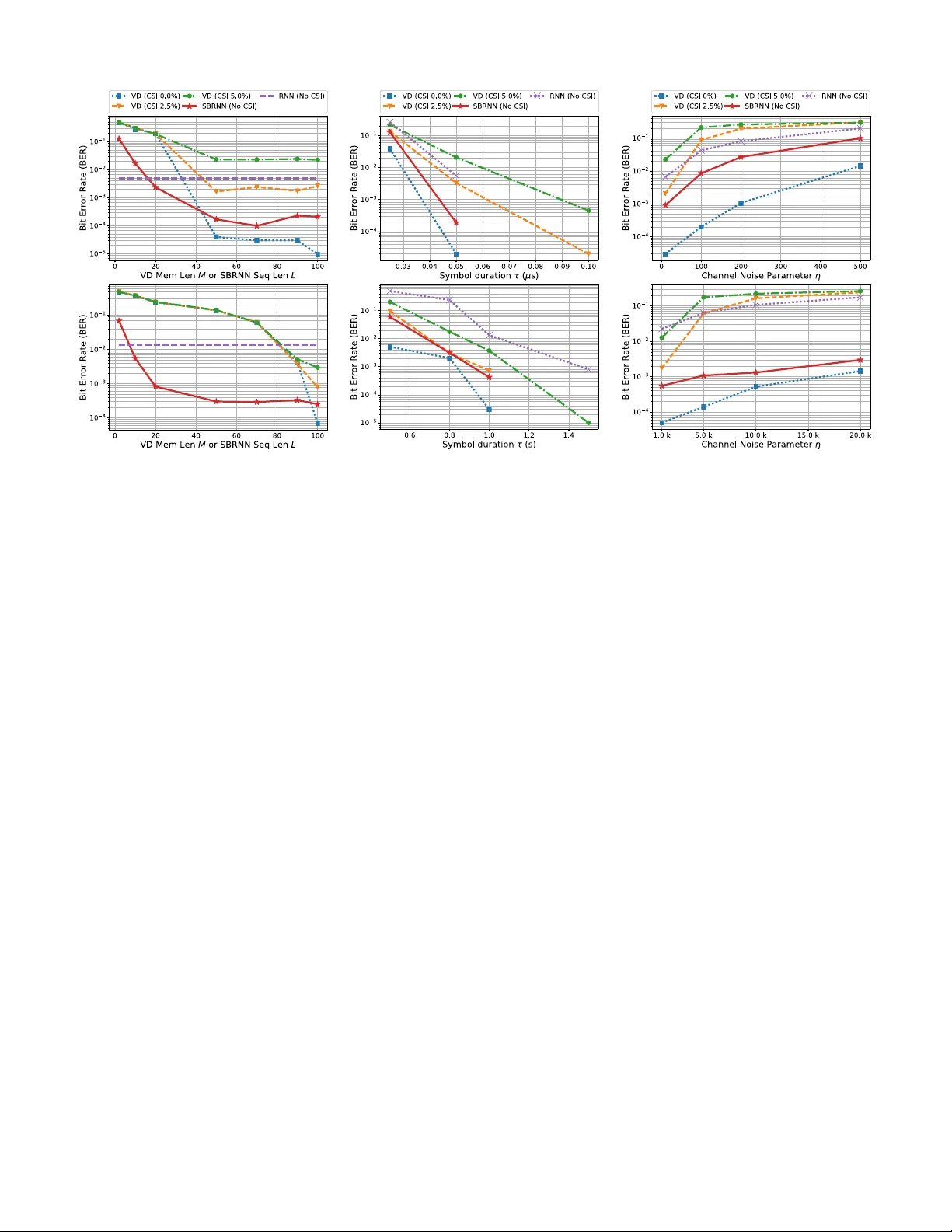
1 Neural Network Detection of Data Sequences in Communication Systems Nariman Farsad, Member , IEEE, and Andrea Goldsmith, F ellow , IEEE Abstract —W e consider detection based on deep learning, and show it is possible to train detectors that perf orm well without any knowledge of the underlying channel models. Moreov er , when the channel model is known, we demonstrate that it is possible to train detectors that do not require channel state inf ormation (CSI). In particular , a technique we call a sliding bidirectional recurr ent neural netw ork (SBRNN) is proposed for detection where, after training, the detector estimates the data in real- time as the signal stream arri ves at the recei ver . W e evaluate this algorithm, as well as other neural network (NN) architectur es, using the Poisson channel model, which is applicable to both optical and molecular communication systems. In addition, we also evaluate the performance of this detection method applied to data sent over a molecular communication platform, where the channel model is difﬁcult to model analytically . W e show that SBRNN is computationally efﬁcient, and can perform detection under v arious channel conditions without kno wing the underlying channel model. W e also demonstrate that the bit err or rate (BER) performance of the proposed SBRNN detector is better than that of a V iterbi detector with imperfect CSI as well as that of other NN detectors that have been previously proposed. Finally , we show that the SBRNN can perform well in rapidly changing channels, where the coher ence time is on the order of a single symbol duration. Index T erms —Machine learning, deep lear ning, supervised learning, communication systems, detection, optical communi- cation, free-space optical communication, molecular communica- tion. I . I N T RO D U C T I O N O NE of the important modules in reliable recov ery of data sent ov er a communication channel is the detection algorithm, where the transmitted signal is estimated from a noisy and corrupted version observed at the recei ver . The design and analysis of this module has traditionally relied on mathematical models that describe the transmission process, signal propagation, recei ver noise, and man y other components of the system that affect the end-to-end signal transmission and reception. Most communication systems today conv ey data by embedding it into electromagnetic (EM) signals, which lend themselv es to tractable channel models based on a simpliﬁcation of Maxwell’ s equations. Howe ver , there are cases where tractable mathematical descriptions of the channel are elusiv e, either because the EM signal propagation is very complicated or when it is poorly understood. In addition, there are communication systems that do not use EM wa ve signalling and the corresponding communication channel models may be unknown or mathematically intractable. Some examples of the latter are underwater communication using Nariman Farsad and Andrea Goldsmith are with the Department of Electrical Engineering, Stanford University , Stanford, CA, 94305. Emails: nfarsad@stanford.edu, andrea@wsl.stanford.edu. This work was funded by the NSF Center for Science of Information grant NSF-CCF-0939370, and ONR grant N00014-18-1-2191. acoustic signals [1] as well as molecular communication, which relies on chemical signals to interconnect tin y de vices with sub-millimeter dimensions in en vironments such as inside the human body [2]–[5]. Even when the underlying channel models are known, since the channel conditions may change with time, many model-based detection algorithms rely on the estimation of the instantaneous channel state information (CSI) (i.e., channel model parameters) for detection. T ypically , this is achiev ed by transmitting and receiving a predesigned pilot sequence, which is known by the receiver , for estimating the CSI. Howe ver , this estimation process entails o verhead that decreases the data transmission rate. Moreover , the accurac y of the estimation may also affect the performance of the detection algorithm. In this paper , we in vestigate ho w different techniques from artiﬁcial intelligence and deep learning [6]–[8] can be used to design detection algorithms for communication systems that learn directly from data. W e show that these algorithms are robust enough to perform detection under changing channel conditions, without knowing the underlying channel models or the CSI. This approach is particularly effecti ve in emerging communication technologies, such as molecular communica- tion, where accurate models may not exist or are difﬁcult to deriv e analytically . For example, tractable analytical channel models for signal propagation in molecular communication channels with multiple reactiv e chemicals hav e been elu- siv e [9]–[11]. Some examples of machine learning tools applied to de- sign problems in communication systems include multiuser detection in code-division multiple-access (CDMA) systems [12]–[15], decoding of linear codes [16], design of new modulation and demodulation schemes [17], [18], detection and channel decoding [19]–[24], and estimating channel model parameters [25], [26]. A recent survey of machine learning techniques applied to communication systems can be found in [27]. The approach taken in most of these pre vious w orks was to use machine learning to improve one component of the communication system based on the knowledge of the underlying channel models. Our approach is different from prior works since we assume that the mathematical models for the communication channel are completely unknown. This is moti vated by the recent success in using deep neural networks (NNs) for end-to-end system design in applications such as image classiﬁcation [28], [29], speech recognition [30]–[32], machine translation [33], [34], and bioinformatics [35]. For example, Figure 1 highlights some of the similarities between speech recognition, where deep NNs hav e been v ery successful at improving the detector’ s performance, and digital communication systems 2 words ! " , ! $ , ⋯ , ! & Signal Propagation ' " ' $ ⋯ ' & Detection Algorithm estimated words ! ( " , ! ( $ , ⋯ , ! ( & data bits ) " , ) $ , ⋯ , ) & Signal Propagation Detection Algorithm estimated bits ) * " , ) * $ , ⋯ , ) * & data bits ) " , ) $ , ⋯ , ) & Signal Propagation Detection Algorithm estimated bits ) * " , ) * $ , ⋯ , ) * & chemical emitter chemical receiver ' " ' $ ⋯ ' & Fig. 1: Similarities between speech recognition and digital communication systems. for wireless and molecular channels. As indicated in the ﬁgure, for speech processing, the transmitter is the speaker , the transmission symbols are words, and the carrier signal is acoustic wav es. At the recei ver the goal of the detection algorithm is to recov er the sequence of transmitted w ords from the acoustic signals that are recei ved by the microphone. Similarly , in communication systems, such as wireless or molecular communications, the transmitted symbols are bits and the carrier signals are EM wav es or chemical signals. At the receiver the goal of the detection algorithm is to detect the transmitted bits from the received signal. One important dif fer- ence between communication systems and speech recognition is the size of transmission symbol set, which is signiﬁcantly larger for speech. Motiv ated by this similarity , in this work we in vestigate how techniques from deep learning can be used to train a detection algorithm from samples of transmitted and receiv ed signals. W e demonstrate that, using known NN architectures such as a recurrent neural network (RNN), it is possible to train a detec- tor without any knowledge of the underlying system model. In this approach, the recei ver goes through a training phase where a NN detector is trained using kno wn transmission signals. W e also propose a real-time NN sequence detector, which we call the sliding bidir ectional RNN (SBRNN) detector , that detects the symbols corresponding to a data stream as they arriv e at the destination. W e demonstrate that if the SBRNN detector or the other NN detectors considered in this work are trained using a di verse dataset that contains sequences transmitted under different channel conditions, the detectors will be robust to changing channel conditions, eliminating the need for instantaneous CSI estimation for the speciﬁc channels considered in this work. At ﬁrst glance, the training phase in this approach may seem like an extra ov erhead. Howe ver , if the underlying channel models are kno wn, then the models could be used off- line to generate training data under a div erse set of channel conditions. W e demonstrate that using this approach, it is possible to train our SBRNN algorithm such that it would not require any instantaneous CSI. Another important beneﬁt of using NN detectors in general is that they return likelihoods for each symbol. These likelihoods can be fed directly from the detector into a soft decoding algorithm such as the belief propagation algorithm without requiring a dedicated module to con vert the detected symbols into likelihoods. T o e valuate the performance of NN detectors, we ﬁrst use the Poisson channel model, a common model for optical channels and molecular communication channels [36]–[41]. W e use this model to compare the performance of the NN detection to the V iterbi detector (VD). W e show that for channels with long memories the SBRNN detection algorithm is computationally more efﬁcient than the VD. Moreover , the VD requires CSI estimation, and its performance can degrade if this estimate is not accurate, while the SBRNN detector can perform detection without the CSI, even in a channel with changing conditions. W e sho w that the bit error rate (BER) performance of the proposed SBRNN is better than the VD with CSI estimation error and it outperforms other well- known NN detectors such as the RNN detector . As another performance measure, we use the experimental data collected by the molecular communication platform presented in [42]. The mathematical models underlying this experimental plat- form are currently unkno wn. W e demonstrate that the proposed SBRNN algorithm can be used to train a sequence detector directly from limited measurement data. W e also demonstrate that this approach perform signiﬁcantly better than the detector used in previous experimental demonstrations [43], [44], as well as other NN detectors. The rest of the paper is organized as follows. In Section II we present the problem statement. Then, in Section III, de- tection algorithms based on NNs are introduced including the ne wly proposed SBRNN algorithm. The Poisson channel model and the VD are introduced in Section IV. The perfor- mance of the NN detection algorithms are ev aluated using this channel model and are compared against the VD in Section V. In Section VI, the performance of NN detection algorithms are ev aluated using a small data set that is collected via an 3 data Source' Encoder Channel' Encoder Signal' T ransmission ! 1 , ! 2 , …& Signal' Propagation Signal' Reception ' 1 , ' 2 , …& Chan nel Detection' Algorithm ! ( 1 , ! ( 2 , …& Channel' Decoder Source' Decoder Recovered. Data Fig. 2: Block diagram for digital communication systems. experimental platform. Concluding remarks are provided in Section VII. I I . P RO B L E M S T AT E M E N T In a digital communication system data is con verted into a sequence of symbols for transmission over the channel. This process is typically carried out in two steps: in the ﬁrst step, source coding is used to compress or represent the data using symbols or bits; in the second step, channel coding is used to introduce extra redundant symbols to mitigate the errors that may be introduced as part of the transmission and reception of the data [45]. Let S = { s 1 , s 2 , · · · , s m } be the ﬁnite set of symbols that could be sent by the transmitter, and x k ∈ S be the k th symbol that is transmitted. The channel coding can be designed such that the individual symbols in a long sequence are drawn according to the probability mass function (PMF) P X ( x ) . The signal that is observed at the destination is noisy and corrupted due to the perturbations introduced as part of transmission, propagation, and reception processes. W e refer to these three processes collectiv ely as the communication channel or simply the c hannel . Let the random vector y k of length ` be the observed signal at the destination during the k th transmission. Note that the observed signal y k is typically a vector while the transmitted symbol x k is typically a scalar . A detection algorithm is then used to estimate the transmitted symbols from the observed signal at the receiver . Let ˆ x k be the symbol that is estimated for the k th transmitted symbol x k . After detection, the estimated symbols are passed to a channel decoder to correct some of the errors in detection, and then to a source decoder to recov er the data. All the components of a communication system, shown in Figure 2, are designed to ensure reliable data transfer . T ypically , to design these modules, mathematical channel models are required, which describe the relationship between the transmitted symbols and the observed signal through P model ( y 1 , y 2 , · · · | x 1 , x 2 , · · · ; Θ ) , (1) where Θ are the model parameters. Some of these parameters can be static (constants that do not change with channel conditions) and some of them can dynamically change with channel conditions over time. In this work, model parameters are considered to be the parameters that change with time. Hence, we use the terms model parameter and instantaneous CSI interchangeably . Using this model, the detection can be performed through symbol-by-symbol detection, where ˆ x k is estimated from y k , or using sequence detection where the sequence ˆ x k , ˆ x k − 1 , · · · , ˆ x 1 is estimated from the sequence y k , y k − 1 , · · · , y 1 1 . As an example, for a simple channel with no intersymbol interference (ISI), giv en by the channel model P model ( y k | x k ; Θ ) , and a kno wn PMF for the transmission symbols P X ( x ) , a maximum a posteriori estimation (MAP) algorithm can be devised as ˆ x k = arg max x ∈S P model ( y k | x ; Θ ) P X ( x ) . (2) Therefore for detection, both the model and the parameters of the model Θ , which may change with time, are required. For this reason, many detection algorithms periodically estimate the model parameters (i.e., the CSI) by transmitting known symbols and then using the observed signals at the receiver for CSI estimation [46]. This extra overhead leads to a decrease in the data rate. One way to avoid CSI estimation is by using blind detectors. These detectors typically assume a particular probability distribution o ver Θ , and perform the detection without estimating the instantaneous CSI at the cost of higher probability of error . Howe ver , estimating the joint distribution ov er all model parameters Θ can also be difﬁcult, requiring a large amount of measurement data under various channel conditions. One of the problems we consider in this work is whether NN detectors can learn this distribution during training, or learn to simultaneously estimate the CSI and detect the symbols. This approach results in a rob ust detection algorithm that performs well under different and changing channel conditions without an y kno wledge of the channel models or their parameters. When the underlying channel models do not lend them- selves to computationally efﬁcient detection algorithms, or are partly or completely unkno wn, the best approach to designing detection algorithms is unclear . For example, in communica- tion channels with memory , the comple xity of the optimal VD increases exponentially with memory length, and quickly becomes infeasible for systems with long memory . Note that the VD also relies on the knowledge of the channel model in terms of its input-output transition probability . As another example, tractable channel models for molecular communica- tion channels with multiple reactiv e chemicals are unknown [9]–[11]. W e propose that in these scenarios, a data driven approach using deep learning is an ef fectiv e w ay to train detectors to determine the transmitted symbols directly using known transmission sequences. I I I . D E T E C T I O N U S I N G D E E P L E A R N I N G Estimating the transmitted symbol from the receiv ed signals can be performed using NN architectures through supervised learning. This is achie ved in two phases. First, a training 1 Note that the sequence of symbols ˆ x k , ˆ x k − 1 , · · · , ˆ x 1 can also be esti- mated from y k + ` , y k + ` − 1 , · · · , y 1 for some integer ` . Howev er , to keep the notation simpler, without loss of generality we assume ` = 0 . 4 Dense Layer 1 Dense Layer 2 ! " # $ Dense Layer (softmax) % # & ' ( " Conv Layer(s) Pooling Layer ! " Dense Layer (softmax) % ' ( " Symbol-by- Symbol Detec . (a) (b) Sequence Detection (c) RNN Layer 1 RNN Layer 2 Dense softmax % ' ( ") $ ! ") $ RNN Layer 1 RNN Layer 2 Dense softmax % ' ( " ! " * ") $ +& , * ") $ +$ , - * " +& , * " +$ , RNN Layer 1 RNN Layer 2 Dense softmax % ' ( ". $ ! ". $ * ". $ +& , * ". $ +$ , * ". & +& , * ". & +$ , - RNN - F Layer 1 RNN - B Layer 1 Dense softmax % ' ( $ ! $ RNN - F Layer 1 RNN - B Layer 1 Dense softmax % ' ( & ! & * / 0 +$ , * 1 2) $ +$ , RNN - F Layer 1 RNN - B Layer 1 Dense softmax % ' ( 3 ! 3 * / $ +$ , * / 2) $ +$ , Merge * / & +$ , - Merge * 1 $ +$ , - Merge * 1 2) & +$ , * 1 0 +$ , - - (d) Fig. 3: Different neural network architectures for detection. dataset is used to train the NN of ﬂine. Once the network is trained, it can be deployed and used for detection. Note that the training phase is performed once ofﬂine, and therefore, it is not part of the detection process after deployment. W e start this section by describing the training process. A. T raining the Detector Let m = |S | be the cardinality of the symbol set, and let p k be the one-of- m representation of the symbol transmitted during the k th transmission, giv en by p k =  1 ( x k = s 1 ) , 1 ( x k = s 2 ) , · · · , 1 ( x k = s m )  | , (3) where 1 ( . ) is the indicator function. Therefore, the element corresponding to the symbol that is transmitted is 1, and all other elements of p k are 0. Note that this is also the PMF of the transmitted symbol during the k th transmission where, at the transmitter , with probability 1, one of the m symbols is transmitted. Also note that the length of the v ector p k is m , which may be different from the length of the vector of the observation signal y k at the destination. The detection algorithm goes through two phases. In the ﬁrst phase, known sequences of symbols from S are transmitted repeatedly and receiv ed by the system to create a set of training data. The training data can be generated by selecting the transmitted symbols randomly according to a PMF , and generating the corresponding recei ved signal using mathemat- ical models, simulations, experimental measurements, or ﬁeld measurements. Let P K = [ p 1 , p 2 , · · · , p K ] be a sequence of K consecuti vely transmitted symbols (in the one-of- m encoded representation), and Y K = [ y 1 , y 2 , · · · , y K ] the corresponding sequence of observed signals at the destination. Then, the training dataset is represented by { ( P (1) K 1 , Y (1) K 1 ) , ( P (2) K 2 , Y (2) K 2 ) , · · · , ( P ( n ) K n , Y ( n ) K n ) } , (4) which consists of n training samples, where the i th sample has K i consecutiv e transmissions. This dataset is then used to train a deep NN classiﬁer that maps the receiv ed signal y k to one of the transmission symbols in S . The input to the NN can be the raw observed signals y k , or a set of features r k extracted from the recei ved signals. The NN outputs are the v ectors ˆ p k = NN ( y k ; W ) , where W are the parameters of the NN. Using the abov e interpretation of p k as a probability vector , ˆ p k are the estimations of the probability of x k giv en the observations and the parameters of the NN. Note that this output is also useful for soft decision channel decoders (i.e., decoders where the decoder inputs are PMFs), which are typically the next module after detection as shown in Figure 2. If channel coding is not used, the symbol is estimated using ˆ x k = arg max x k ∈S ˆ p k . During the training, kno wn transmission sequences of sym- bols are used to ﬁnd the optimal set of parameters for the NN W ∗ such that W ∗ = arg min W L ( p k , ˆ p k ) , (5) where L is the loss function. This optimization algorithm is typically solved using the training data, v ariants of stochastic gradient decent, and back propagation [7]. Since the output of the NN is a PMF , the cross-entropy loss function can be used for this optimization [7]: L cross = H ( p k , ˆ p k ) = H ( p k ) + D KL ( p k k ˆ p k ) , (6) where H ( p k , ˆ p k ) is the cross entropy between the correct PMF and the estimated PMF , and D KL ( . k . ) is the Kullback- Leibler div ergence [47]. Note that minimizing the loss is equiv alent to minimizing the cross-entropy or the Kullback- Leibler div ergence distance between the true PMF and the one estimated based on the NN. It is also equiv alent to maximizing the log-likelihoods. Therefore, during the training, known transmission data are used to train a detector that maximizes log-likelihoods . Using Bayes’ theorem, it is easy to show that minimizing the loss is equiv alent to maximizing (2). W e now discuss how several well-known NN architectures can be used for symbol-by-symbol detection and for sequence detection. B. Symbol-by-Symbol Detectors The most basic NN architecture that can be employed for detection uses se veral fully connected NN layers followed by a ﬁnal softmax layer [6], [7]. The input to the ﬁrst layer is the observed signal y k or the feature v ector r k , which is selecti vely extracted from the observed signal through preprocessing. The output of the ﬁnal layer is of length m (i.e., the cardinality the symbol set), and the acti vation function for the ﬁnal layer is the softmax activ ation. This ensures that the output of the layer ˆ p k is a PMF . Figure 3(a) shows the structure of this NN. A more sophisticated class of NNs that is used in process- ing complex signals such as images is a con volution neural 5 network (CNN) [6], [48], [49]. Essentially , the CNN is a set of ﬁlters that are trained to extract the most relev ant features for detection from the receiv ed signal. The ﬁnal layer in the CNN detector is a dense layer with output of length m , and a softmax activ ation function. This results in an estimate ˆ p k from the set of features that are extracted by the con volutional layers in the CNN. Figure 3(b) shows the structure of this NN. For symbol-by-symbol detection the estimated PMF ˆ p k is giv en by ˆ x k = [ P NN ( x k = s 1 | y k ) , P NN ( x k = s 2 | y k ) , · · · , P NN ( x k = s m | y k ) ] | , (7) where P NN is the probability of estimating each symbol based on the NN model used. The better the structure of the NN at capturing the physical channel characteristics based on P model in (1), the better this estimate and the results. C. Sequence Detectors The symbol-by-symbol detector cannot tak e into account the effects of ISI between symbols 2 . In this case, sequence detec- tion can be performed using recurrent neural networks (RNN) [6], [7], which are well established for sequence estimation in different problems such as neural machine translation [33], speech recognition [30], or bioinformatics [35]. The estimated ˆ p k in this case is gi ven by ˆ p k =      P RNN ( x k = s 1 | y k , y k − 1 , · · · , y 1 ) P RNN ( x k = s 2 | y k , y k − 1 , · · · , y 1 ) . . . P RNN ( x k = s m | y k , y k − 1 , · · · , y 1 )      , (8) where P RNN is the probability of estimating each symbol based on the NN model used. In this work, we use long short-term memory (LSTM) networks [50], which hav e been extensiv ely used in many applications. Figure 3(c) shows the RNN structure. One of the main beneﬁts of this detector is that after training, similar to a symbol-by-symbol detector , it can perform detection on any data stream as it arriv es at the recei ver . This is because the observations from previous symbols are summarized as the state of the RNN, which is represented by the vector h k . Note that the observed signal during the j th transmission slot, y j where j > k , may carry information about the k th symbol x k due to delays in signal arri val which results in ISI. Howe ver , since RNNs are feed-forward only , during the estimation of ˆ p k , the observation signal y j is not considered. One way to ov ercome this limitation is by using bidirec- tional RNNs (BRNNs), where the sequence of received signals are once fed in the forw ard direction into one RNN cell and once fed in backwards into another RNN cell [51]. The two outputs are then concatenated and may be passed to more bidirectional layers. Figure 3(d) shows the BRNN structure. 2 It is possible to use the received signal from multiple symbols as input to a CNN for detection in the presence of ISI. ! 1 ! # ! $ ! % ! & ! ' ! ( ! ) ! * BRNN Stream of Observed Signals … BRNN BRNN BRNN BRNN BRNN Block Detector Sliding BRNN Detector Fig. 4: The sliding BRNN detector . For a sequence of length L , the estimated ˆ p k for BRNN is giv en by ˆ p k =      P BRNN ( x k = s 1 | y L , y L − 1 , · · · , y 1 ) P BRNN ( x k = s 2 | y L , y L − 1 , · · · , y 1 ) . . . P BRNN ( x k = s m | y L , y L − 1 , · · · , y 1 )      , (9) where k ≤ L . In this work we use the bidirectional LSTM (BLSTM) networks [52]. The BRNN architecture ensures that in the estimation of a symbol, future signal observations are taken into account, thereby ov ercoming the limitations of RNNs. The main trade- off is that as signals from a data stream arrive at the destina- tion, the block length L increases, and the whole block needs to be re-estimated again for each ne w data symbol that is receiv ed. Therefore, this quickly becomes infeasible for long data streams as the length of the data stream can be on the order of tens of thousands to millions of symbols. In the next section we present a ne w technique to solv e this issue. D. Sliding BRNN Detector Since the data stream that arriv es at the receiv er can hav e any arbitrary length, it is not desirable to detect the whole sequence for each ne w symbol that arriv es, as the sequence length could grow arbitrarily large. Therefore, we ﬁx the maximum length of the BRNN. Ideally , the length must be at least the same size as the memory length of the channel. Howe ver , if this is not known in adv ance, the BRNN length can be treated as a hyperparameter to be tuned during training. Let L be the maximum length of the BRNN. Then during training, blocks of ` ≤ L consecutiv e transmissions are used for training. Note that sequences of different lengths could be used during training as long as all sequence lengths are smaller than or equal to L . After training, the simplest scheme would be to detect the stream of incoming data in ﬁxed blocks of length ` ≤ L as sho wn in the top portion of Figure 4. The main drawback here is that the symbols at the end of each block may affect the symbols in the next block, and this relation is not captured in this scheme. Another issue is that ` consecutive symbols must be receiv ed before detection can be performed. The top portion of Figure 4 shows this scheme for ` = 3 . T o overcome these limitations, inspired by some of the techniques used in speech recognition [53], we propose a dy- namic programing scheme we call the sliding BRNN (SBRNN) detector . In this scheme the ﬁrst ` ≤ L symbols are detected using the BRNN. Then as each ne w symbol arri ves at the destination, the position of the BRNN slides ahead by one 6 symbol. Let the set J k = { j | j ≤ k ∧ j + L > k } be the set of all v alid starting positions for a BRNN detector of length L , such that the detector overlaps with the k th symbol. For example, if L = 3 and k = 4 , then j = 1 is not in the set J k since the BRNN detector overlaps with symbol positions 1, 2, and 3, and not the symbol position 4. Let ˆ p ( j ) k be the estimated PMF for the k th symbol, when the start of the sliding BRNN is on j ∈ J k . The ﬁnal PMF corresponding to the k th symbol is giv en by the weighted sum of the estimated PMFs for each of the relev ant windo ws: ˆ p k = 1 |J k | X j ∈J k ˆ p ( j ) k . (10) One of the main beneﬁts of this approach is that, after the ﬁrst L symbols are receiv ed and detected, as the signal corresponding to a new symbol arriv es at the destination, the detector immediately estimates that symbol. The detector also updates its estimate for the pre vious L − 1 symbols dynamically . Therefore, this algorithm is similar to a dynamic programming algorithm. The bottom portion of Figure 4 illustrates the sliding BRNN detector . In this example, after the ﬁrst 3 symbols arriv e, the PMF for the ﬁrst three symbols, i ∈ { 1 , 2 , 3 } , is giv en by ˆ p i = ˆ p (1) i . When the 4th symbol arri ves, the estimate of the ﬁrst symbol is unchanged, but for i ∈ { 2 , 3 } , the second and third symbol estimates are updated as ˆ x i = 1 2 ( ˆ x (1) i + ˆ x (2) i ) , and the 4th symbol is estimated by ˆ p 4 = ˆ p (2) 4 . Note that although in this paper we assume that the weights of all ˆ p ( j ) k are the same (i.e., 1 |J k | ), the algorithm can use different weights. Moreover , the complexity of the SBRNN increases linearly with the length of the BRNN windo w , and hence with the memory length. T o ev aluate the performance of all these NN detectors, we use both the Poisson channel model (a common model for optical and molecular communication systems) as well as an experimental platform for molecular communication where the underlying model is unknown [42]. The sequel discusses more details of the Poisson model and experimental platform, and how they were used for performance analysis of our proposed techniques. I V . T H E P O I S S O N C H A N N E L M O D E L The Poisson channel has been used extensiv ely to model different communication systems in optical and molecular communication [36]–[41]. In these systems, information is encoded in the intensity of the photons or particles released by the transmitter and decoded from the intensity of photons or particles observed at the receiv er . In the rest of this section, we refer to the photons, molecules, or particles simply as particles . W e now describe this channel, and a VD for the channel. In our model it is assumed that the transmitter uses on-off- keying (OOK) modulation, where the transmission symbol set is S = { 0 , 1 } , and the transmitter either transmits a pulse with a ﬁxed intensity to represent the 1-bit or no pulse to represent the 0-bit. Note that OOK modulation has been considered in many pre vious works on optical and molecular communication ! " ! " ! " ! " ! " ! " ! " ! " ! " ! " Fig. 5: A sample system response for optical and molecular channels. Left: Optical channel with λ ( t ) for N = 1 , κ OP = 1 , α = 2 , β = 0 . 2 , τ = 0 . 2 µ s, and ω = 20 MS/s. At τ = 0 . 2 µ s, much of the intensity from the current transmission will arrive during future symbol intervals. Right: Molecular channel with κ MO = 1 , c = 8 , µ = 40 , τ = 2 s, and ω = 2 S/s. Molecular channel response has a loner tail than optical channel. and has been shown to be the optimal input distribution for a large class of Poisson channels [54]–[56]. Later in Section V -D, we extend the results to larger symbol sets by considering the general m level pulse amplitude modulation ( m -P AM), where information is encoded in m amplitudes of the pulse transmissions. Note that OOK is a special case of this modulation scheme with m = 2 . Let τ be the symbol interval, and x k ∈ S the symbol corresponding to the k th transmission. W e assume that the transmitter can measure the number of particles that arriv e at a sampling rate of ω samples per second. Then the number of samples in a giv en symbol duration is giv en by a = ω τ , where we assume that a is an integer . Let λ ( t ) be the system response to a transmission of the pulse corresponding to the 1-bit. For optical channels, the system response is proportional to the Gamma distribution, and given by [57]–[59]: λ OP ( t ) = ( κ OP β − α t α − 1 Γ( α ) exp( − t/β ) t > 0 0 t ≤ 0 , (11) where κ OP is the proportionality constant, and α and β are parameters of the channel, which can change over time. For molecular channels, the system response is proportional to the in verse Gaussian distribution [39], [40], [60], [61] given by: λ MO ( t ) = ( κ MO p c 2 π t 3 exp h − c ( t − µ ) 2 2 µ 2 t i t > 0 0 t ≤ 0 , (12) where κ MO is the proportionality constant, and c and µ are parameters of the channel, which can change over time. Since the recei ver samples the data at a rate of ω , for k ∈ N and j ∈ { 1 , 2 , · · · , a } , let λ k [ j ] , λ  j + k a ω  (13) be the av erage intensity observed during the j th sample of the k th symbol in response to the transmission pulse corresponding to the 1-bit. Figure 5 sho ws the system response for both optical and molecular channels. Although for optical channels the symbol duration is many orders of magnitude smaller than for molecular channels, the system responses are very similar 7 0 1 0 1 1 1 0 0 1 1 1 0 0 0 Fig. 6: The observed signal for the transmission of the bit sequence 10101100111000 for κ MO = 100 , c = 8 , µ = 40 , τ = 1 , ω = 100 Hz, and η = 1 . in shape. Some notable differences are a faster rise time for the optical channel, and a longer tail for the molecular channel. The system responses are used to formulate the Poisson channel model. In particular, the intensity that is observ ed during the j th sample of the k th symbol is distrib uted according to y k [ j ] ∼ P k X i =0 x k − i λ i [ j ] + η ! , (14) where P ( ξ ) = ξ y e − ξ y ! is the Poisson distribution, and η is the mean of an independent additi ve Poisson noise due to background interference and/or the recei ver noise 3 . Using this model, the signal that is observed by the receiv er, for any sequence of bit transmissions, can be generated as illustrated in Figure 6. This signal has a similar structure to the signal observed using the experimental platform in [43, see Figure 13], although this analytically-modeled signal exhibits more noise. The model parameters (i.e., the CSI) for the Poisson channel model are Θ OP = [ α, β , η ] and Θ MO = [ c, µ, η ] , respectiv ely for optical and molecular channels. In this work, we assume that the sampling rate ω , and the proportionality constants κ OP and κ MO are ﬁx ed and are not part of the model parameters. Note that α and β can change ov er time due to atmospheric turbulence or mobility . Similarly , c and µ are functions of the distance between the transmitter and the receiv er, ﬂow velocity , and the dif fusion coef ﬁcient, which may change ov er time, e.g., due to v ariations in temperature and pressure [5]. The background noise η may also change with time. Note that although the symbol interv al τ may be changed to increase or decrease the data rate, both the transmitter and recei ver must agree on the v alue of τ . Thus, we assume that the value of τ is al ways known at the recei ver , and therefore, it is not part of the CSI. In the next subsection, we present the optimal VD, 3 Note that η is the noise term that is typically used in the Poisson channel model. In the optical communication literature this noise is also known as the dark current [36]–[38]. The noise is due to imperfect recei ver , or background noise (due to ambient optical noise or molecules that may exist in the en vironment). assuming that the recei ver knows all the model parameters Θ OP and Θ MO perfectly . A. The V iterbi Detector The VD assumes a certain memory length M where the cur - rent observed signal is affected only by the past M transmitted symbols. In this case (14) becomes y k [ j ] ∼ P x k λ 0 [ j ] + M X l =1 x k − l λ l [ j ] + η ! . (15) Since the marginal distribution of the j th sample of the k th symbol is Poisson distributed according to (15), giv en the model parameters Θ pois , we have P ( y k | x k − M ,x k − M +1 , · · · , x k , Θ pois ) = a Y j =1 P ( y k [ j ] | x k − M , x k − M +1 , · · · , x k , Θ pois ) . (16) This is because, giv en the model parameters as well as the current symbol and the previous M symbols, the samples within the current bit interval are generated independently and distributed according to (15). Note that (16) holds only if the memory length M is known perfectly . If the estimate of M is inaccurate, then (16) is also inaccurate. Let V = { v 0 , v 1 , · · · , v 2 M − 1 } be the set of states in the trellis of the VD, where the state v u corresponds to the previous M transmitted bits [ x − M , x − M +1 , · · · , x − 1 ] form- ing the binary representation of u . Let ˆ x k , 1 ≤ k ≤ K be the information bits to be estimated. Let V k,u be the state corresponding to the k th symbol interv al, where u is the binary representation of [ ˆ x k − M , ˆ x k − M +1 , · · · , ˆ x k − 1 ] . Let L ( V k,u ) denote the log-likelihood of the state V k,u . For a state V k +1 ,u = [ ˆ x k − M +1 , ˆ x k − M +2 , · · · , ˆ x k ] , there are two states in the set { V k,i } 2 M − 1 i =0 that can transition to V k +1 ,u : u 0 = b u 2 c , (17) u 1 = b u 2 c + 2 M − 1 , (18) where b . c is the ﬂoor function. Let the binary vector b u 0 = [0 , ˆ x k − M +1 , ˆ x k − M +2 , · · · , ˆ x k − 1 ] be the binary representation of u 0 and similarly b u 1 the binary representation of u 1 . The log-likelihoods of each state in the ne xt symbol slot are updated according to L ( V k +1 ,u ) = max[ L ( V k,u 0 ) + L ( V k,u 0 , V k +1 ,u ) , L ( V k,u 1 ) + L ( V k,u 1 , V k +1 ,u )] , (19) where L ( V k,u i , V k +1 ,u ) , i ∈ { 0 , 1 } , is the log-likelihood increment of transitioning from state V k,u i to V k +1 ,u . Let Λ u i ,u [ j ] = ( u mo d 2) λ 0 [ j ] + M X l =1 b u i [ M − l + 1] λ l [ j ] + η . (20) 8 Using the PMF of the Poisson distribution, (15), (16), and (20) we hav e L ( V k,u i , V k +1 ,u ) = − a X j =1 Λ u i ,u [ j ] + a X j =1 log( Λ u i ,u [ j ]) y k [ j ] , (21) where the extra term − P a j =1 log( y k [ j ]!) is dropped since it will be the same for both transitions from u 0 and u 1 . Using these transition probabilities and setting the L ( V 0 , 0 ) = 0 and L ( V 0 ,u ) = −∞ , for u 6 = 0 , the most lik ely sequence ˆ x k , 1 ≤ k ≤ K , can be estimated using the V iterbi algorithm [62]. When the memory length is long, it is not computationally feasible to consider all the states in the trellis as they grow exponentially with memory length. Therefore, in this w ork we implement the V iterbi beam search algorithm [63]. In this scheme, at each time slot, only the transition from the previous N states with the largest log-likelihoods are considered. When N = 2 M , the V iterbi beam search algorithm reduces to the traditional V iterbi algorithm. W e now ev aluate the performance of NN detectors using the Poisson channel model. V . E V A L U A T I O N B A S E D O N P O I S S O N C H A N N E L In this section we ev aluate the performance of the proposed SBRNN detector based on the Poisson channel model, and in the next section we use the experimental platform de vel- oped in [42] to demonstrate that the SBRNN detector can be implemented in practice to perform real-time detection. The rest of this section is or ganized as follo ws. First, we describe the training procedure and the simulation setup in Section V -A. Then, in Section V -B, we ev aluate the effects of L max and M , the symbol duration, and noise on the BER performance. In particular, in this section we demonstrate that SBRNN detection is resilient to changes in symbol duration and noise, and outperforms VD with perfect CSI if the memory length M is not estimated correctly . In Section V -C, the performance of the SBRNN detector and VD are ev aluated for different channel parameters. T o show that the SBRNN algorithm works on larger symbol sets (i.e., higher order modulations), in section V -D we consider an optical channel that uses m -P AM, m > 2 , instead of OOK (i.e., 2-P AM). W e also demonstrate that although the training is performed on transmission sequences of length 100, the SBRNN can generalize to longer transmission sequences. The effects of the RNN cell type is also ev aluated and it is demonstrated that LSTM cells achieve the best BER performance. The performance of the SBRNN in rapidly changing channels is ev aluated in Section V -E, and the comple xity of this algorithm compared to the VD is discussed in Section V -F. T able I summarizes all the results that will be presented in this section. T ABLE I: Summary of the results to be presented in this section. sec. Chan T ypes Evaluates B Optical/Molecular (OOK) sequence length, symbol duration, noise C Optical/Molecular (OOK) channel parameters (i.e., impulse response) D Optical ( m -P AM) symbol size, transmission length, RNN type E Optical/Molecular (OOK) rapidly changing channels T ABLE II: Performance of the VD beam search as function of N . The optical channel results is obtained using Θ OP = [ β = 0 . 2 , η = 1] and τ = 0 . 025 µ s and the molecular channel results using Θ MO = [ c = 8 , µ = 40 , η = 100] and τ = 0 . 5 s. N 10 100 200 500 1000 Opti. VD 0.0% error 0.0466 0.03937 0.03972 0.03906 0.03972 Opti. VD 2.5% error 0.226 0.175 0.17561 0.15889 0.1509 Opti. VD 5.0% error 0.4036 0.385 0.38519 0.39538 0.36 Mole. VD 0.0% error 0.00466 0.00398 0.00464 0.00448 0.00432 Mole. VD 2.5% error 0.0066 0.0055 0.00524 0.0056 0.00582 Mole. VD 5.0% error 0.41792 0.34667 0.30424 0.29314 0.30588 A. T raining and Simulation Procedur e For ev aluating the performance of the SBRNN on the Poisson channel, we consider both the optical channel and the molecular channel. F or the optical channel, we assume that the channel parameters are Θ OP = [ β , η ] , and assume α = 2 and κ OP = 10 . W e use these values for α and κ OP since the y resulted in system responses that resembled the ones presented in [57]–[59]. For the molecular channel the model parameters are Θ MO = [ c, µ, η ] , and κ MO = 10 4 . The value of κ MO was selected to resemble the system response in [43]. For the optical channel we use ω = 2 GS/s and for the molecular channel we use ω = 100 S/s. For the VD algorithm we consider V iterbi with beam search, where only the top N = 100 states with the largest log- likelihoods are kept in the trellis during each time slot. W e also consider two different scenarios for CSI estimation. In the ﬁrst scenario we assume that the detector estimates the CSI perfectly , i.e., the values of the model parameters Θ OP and Θ MO are known perfectly at the receiv er . In practice, it may not be possible to achiev e perfect CSI estimation. In the second scenario we consider the VD with CSI estimation error . Let ζ be a parameter in Θ OP or Θ MO . Then the estimate of this parameter is simulated by ˆ ζ = ζ + Z , where Z is a zero-mean Gaussian noise with a standard deviation that is 2.5% or 5% of ζ . In the rest of this section, we refer to these cases as the VD with 2.5% and 5% error , and the case with perfect CSI as the VD with 0% error . T able II shows the BER performance of the VD for different values of N . It can be seen that N = 100 , which is used in the rest of this section, is sufﬁcient to achie ve good performance with the VD. Both the RNN and the SBRNN detectors use LSTM cells [50], unless speciﬁed otherwise. For the SBRNN, the size of the output is 80. For the RNN, since the SBRNN uses two RNNs, one for the forward direction and one for the backward direction, the size of the output is 160. This ensures that the SBRNN detector and the RNN detector have roughly the same number of parameters. The number of layers used for both detectors in this section is 3. The input to the NNs are a set of normalized features r k extracted from the received signal y k . The feature extraction algorithm is described in the appendix. This feature extraction step normalizes the input, which assists the NNs to learn faster from the data [7]. T o train the RNN and SBRNN detectors, transmitted bits are generated at random and the corresponding recei ved signal is generated using the Poisson model in (14). In particular , the training data consists of many samples of sequences of 100 consecutively transmitted bits and the corresponding 9 (a) (b) (c) optical molecular optical molecular optical molecular Fig. 7: The BER performance comparison of the SBRNN detector , the RNN detector , and the VD. The top plots present the optical channel and the bottom plots present the molecular channel. (a) The BER at various memory lengths M and SBRNN sequence lengths L . T op: Θ OP = [ β = 0 . 2 , η = 1] and τ = 0 . 05 µ s. Bottom: Θ MO = [ c = 10 , µ = 40 , η = 100] and τ = 1 s. (b) The BER at v arious symbol durations for L = 50 and M = 99 . The Θ OP (top) and Θ MO (bottom) are the same as (a). (c) The BER at various noise rates for L = 50 and M = 99 . Except η , all the parameters are the same as those in (a). receiv ed signal. Since in this w ork we focus on uncoded communication, we assume the occurrence of both bits in the transmitted sequence are equiprobable. For each sequence, the CSI are selected at random. Particularly , for the optical channel, for each 100-bit sequence, β ∼ U ( { 0 . 15 , 0 . 16 , 0 . 17 , · · · , 0 . 35 } ) , η ∼ U ( { 1 , 10 , 20 , 50 , 100 , 200 , 500 } ) , τ ∼ U ( { 0 . 025 , 0 . 05 , 0 . 075 , 0 . 1 } ) (all in µ s) , (22) where U ( A ) indicates uniform distribution ov er the set A . Similarly , for the molecular channel, c ∼ U ( { 1 , 2 , · · · , 30 } ) , µ ∼ U ( { 5 , 10 , 15 , · · · , 65 } ) , η ∼ U ( { 1 , 50 , 100 , 500 , 1 k , 5 k , 10 k , 20 k , 30 k , 40 k , 50 k } ) , τ ∼ U ( { 0 . 5 , 1 , 1 . 5 , 2 } ) (all in s) . (23) For the SBRNN training, each 100-bit sequence is randomly broken into subsequences of length L ∼ U ( { 2 , 3 , 4 , · · · , 50 } ) . For all training, the Adam optimization algorithm [64] is used with learning rate of 10 − 3 , and batch size of 500. W e train on 500k sequences of 100 bits. Over the next se veral subsections we ev aluate the perfor- mance of the SBRNN detector and compare it to that of the VD. B. Ef fects of Sequence Length, Symbol Duration, and Noise First, we ev aluate the BER performance with respect to the memory length M used in the VD, and the sequence length L used in the SBRNN. For all the BER performance plots in this section, to calculate the BER, 1000 sequences of 100 random bits are used. Figure 7(a) shows the results for the optical (top plots) and the molecular (bottom plots) channels with the parameters described above. From the results it is clear that the performance of the VD relies heavily on estimating the memory length of the system correctly . W e deﬁne the memory length as the number of symbol durations it takes for the impulse response to be sufﬁciently small such that ISI is negligible or , equi valently , such that increasing the memory length of the detector does not decrease BER signiﬁcantly . For e xample, let λ max be the peak value of the impulse response. Let t σ , 0 < σ < 1 , be the time it takes for impulse response to fall to σ λ max . Then, for the optical channel in Figure 7(a), the time it tak es for the impulse response to fall to 0.01% of λ max is τ 0 . 0001 = 2 . 55 µ s. Therefore, at a symbol duration of τ = 0 . 05 , the memory length is on the order of M ≈ 51 symbols. From Figure 7(a) it can be seen that the BER performance of the VD with perfect CSI does not improve beyond a negligible amount for M > 50 . The molecular channel’ s impulse response has a much longer tail, where at τ = 1 s it takes 382 symbol durations for the impulse response to fall to 0.1% of the peak value λ max . This is e vident in Figure 7(a) where the BER of the VD with perfect CSI always improv es as M increases. Figure 7(a) also demonstrates that if the estimate of M is inaccurate, the SBRNN algorithm outperforms the VD with perfect CSI. W e also observ e that the SBRNN achie ves a better BER when there is a CSI estimation error of 2.5% or more. Note that the RNN detector does not hav e a parameter 10 (a) (b) (c) Fig. 8: The BER performance comparison of the SBRNN detector ( L = 50 ), the RNN detector , and the VD ( M = 99 ). (a) The BER at various β for the optical channel with η = 1 and τ = 0 . 05 µ s. (b) The BER at various c for the molecular channel with µ = 40 , η = 1 , and τ = 1 s. (c) The BER at v arious µ for the molecular channel with c = 10 , η = 1000 , and τ = 1 s. that depends on the memory length and has a signiﬁcantly larger BER compared to the SBRNN. For the optical channel, the RNN detector outperforms the VD with 5% error in CSI estimation. Moreov er, it can seen that the optical channel has a shorter memory length compared to the molecular channel. Remark 1: When the VD has perfect CSI, it can estimate the memory length correctly by using the system response. Howe ver , if there is CSI estimation error , the memory length may not be estimated correctly , and as can be seen in Fig- ure 7(a), this can hav e degrading ef fects on the performance of the VD. Howe ver , in the rest of this section, for all the other VD plots, we use the memory length of 99, i.e., the largest possible memory length in sequences of 100 bits. Although this does not capture the performance degradation that may result from the error in estimating the memory length, as we will show , the SBRNN still achie ves a BER performance that is as good or better than the VD plots with CSI estimation error under various channel conditions. Next we ev aluate the BER for different symbol durations in Figure 7(b). Again we observe that the SBRNN achieves a better BER when there is a CSI estimation error of 2.5% or more. The RNN detector outperforms the VD with 5% CSI estimation error for the optical channel, but does not perform well for the molecular channel. All detectors achiev e zero- error in decoding the 1000 sequences of 100 random bits used to calculate the BER for the optical channel with τ = 0 . 1 µ s. Similarly , for the molecular channel at τ = 1 . 5 s, all detectors except the RNN detector achiev e zero error . Figure 7(c) ev aluates the BER performance at v arious noise rates. The SBRNN achieves a BER performance close to the VD with perfect CSI across a wide range of values. For larger values of η , i.e., lo w signal-to-noise ratio (SNR), both the RNN detector and the SBRNN detector outperform the VD with CSI estimation error . C. Ef fects of Channel P arameters In this section we ev aluate the performance with respect to the channel parameters that affect the system response. Recall that for the optical channel the parameter β affects the system response in (11) (note that here we assume that α = 2 does Fig. 9: The shape the system response for the optical and molecular channel over the range of values in (22) and (23). not change), and for the molecular channel the parameters c and µ af fect the system response in (12). The range of v alues that β is assumed to take is given in (22), and the range of values for c and µ are gi ven in (23). In Figure 8, we ev aluate the performance of the detection al- gorithms with respect to these parameters. Note that in optical and molecular communication these parameters can change rapidly due to atmospheric turbulence, changes in temperature, or changes in the distance between the transmitter and the receiv er . Therefore, estimating these parameters accurately can be challenging. Furthermore, since these parameters change the shape of the system responses they change the memory length as well. Figure 9 sho ws the system response for the optical and molecular channels over the range of values for β , c , and µ in (22) and (23). For a ﬁxed symbol duration, the system response can hav e a considerable effect on the delay spread (i.e., memory order) of the system. From Figure 8, it can be seen that the SBRNN performs as well or better than the VD with an estimation error of 2.5%. Moreov er , for the optical channel, the RNN detector performs better than the VD with 5% estimation error . In all cases, the SBRNN learns to detect ov er the wide range of system responses shown in Figure 9. D. Ef fects of Symbol Set Size, T ransmission Length, and RNN Cell T ype In the previous sections we considered OOK modulation. Howe ver , it is not clear if higher order modulations can be used 11 (a) (b) (c) VD (4-P AM, CSI 0%) VD (OOK, CSI 0%) VD (OOK, CSI 2.5%) VD (4-P AM, CSI 2.5%) Fig. 10: The SER performance comparison of the SBRNN detector ( L = 50 ), and the VD ( M = 99 ) for optical channel with 4-P AM modulation. (a) The SER at various η for the optical channel with β = 0 . 2 and τ = 1 µ s. (b) The SER at various β for the optical channel with η = 10 and τ = 1 µ s. (c) The SER v ersus transmission sequence length for optical channel with OOK modulation ( τ = 0 . 05 µ s, κ OP = 10 , η = 50 ) and 4-P AM modulation ( τ = 0 . 1 µ s, κ OP = 20 , η = 100 ). For both cases β = 0 . 2 and α = 2 . T ABLE III: The SER for different modulations. Modulation SER (Perfect CSI) SER (2.5% CSI Error) OOK 6 . 4 × 10 − 5 9 . 2 × 10 − 3 4-P AM 5 . 3 × 10 − 6 1 . 3 × 10 − 1 8-P AM 1 . 6 × 10 − 4 2 . 5 × 10 − 1 to achiev e better results. In this section we ﬁrst ev aluate the performance of OOK and higher order m -P AM modulations using VD. W e demonstrate that for system parameters under consideration, 4-P AM achieves the best BER performance. Then we demonstrate that the SBRNN detector can be trained on modulations with larger symbol sets. In fact for detection and estimation problems in speech and language processing, where RNNs are extensi vely used, the symbol set (i.e., the number of phonemes or vocabulary size) can be on the order of hundreds to millions of symbols. W e also consider the af fect of different RNN cell types on the symbol error rate (SER) performance and demonstrate that the LSTM cell, which was used in the pre vious sections, achie ves the best performance. Finally , the generalizability of the SBRNN detector to longer transmission sequences is ev aluated where we show that the SBRNN achiev es the same or better SER performance on longer transmission sequences, despite being trained on sequences of length 100. First we compare the performance of OOK, 4-P AM, and 8-P AM modulation, where 2, 4 or 8 amplitude levels are used for encoding 1, 2 or 3 bits of information during each symbol duration. W e assume that amplitudes are equally spaced and include the zero amplitude (i.e., sending no pulse). Because of space limitations, we only focus on the optical channel with the following parameters: OOK with τ = 0 . 05 µ s, κ OP = 10 , η = 50 ; 4-P AM with τ = 0 . 1 µ s, κ OP = 20 , η = 100 ; and 8-P AM with τ = 0 . 15 µ s, κ OP = 30 , η = 150 . For all modulations we use β = 0 . 2 and α = 2 . W e chose these parameters to keep the average transmit power , the data rate, and the peak signal-to-noise ratio (SNR) the same for all modulations. W e then ev aluate the SER using the VD with perfect CSI and the VDs with CSI estimation errors of 2.5%. W e use 500k symbols for ev aluating the SER. T able III sho ws the results. When perfect CSI is av ailable at the receiver , 4-P AM achieves the best SER, while when there is an error in CSI estimation, OOK achiev es the best SER. Note that since the number of bits presented by each symbol of each modulation scheme is different, SER is not the best performance measure. Ho wever , e ven if we assume that each symbol error is due to a single bit error, which results in the best BER possible for 8-P AM, we still observe that 4- P AM achiev es the best BER performance when perfect CSI is av ailable at the receiv er , while OOK achieves the best BER performance when there is CSI estimation error . Since 4-P AM achieves the best BER performance, we trained a new SBRNN detector based on 4-P AM modulation. For training, the channel parameter β is assumed to be uniformly random in the interval β ∈ [0 . 2 , 0 . 35] and the noise parameter η is assumed to be uniformly random in the interval η ∈ [10 , 200] . W e trained three SBRNN detectors based on the LSTM cell, the GR U cell [65], and the v anilla RNN architecture [7]. Figure 10(a)-(b) sho ws the results. As can be seen, the SBRNN with the LSTM cell achie ves a better SER performance compared with the GR U cell and the v anilla RNN cell types. Compared with the VDs, we observe a trend similar to that in OOK modulation: the SBRNN outperforms VD with CSI estimation error , while its performance comes close to the VD with perfect CSI. This demonstrates that the SBRNN algorithm can be e xtended to larger symbol sets. W e last ev aluate the performance of the SBRNN detector ov er longer transmission sequences for OOK and 4-P AM. In particular, for each modulation, two differently trained SBRNN networks are ev aluated. The ﬁrst set of networks are the same networks used to generate Figures 7, 8, and 10(a)- (b). These networks are trained using a data set that contains sample transmissions under various channel conditions. The second set of networks are trained using sample received sig- nals from a very speciﬁc set of channel and noise parameters. Speciﬁcally , the training data is generated using the same set of parameters that are used during testing (i.e., τ = 0 . 05 µ s, κ OP = 10 , η = 50 for OOK and τ = 0 . 1 µ s, κ OP = 20 , η = 100 for 4-P AM). Note that all the SBRNN detectors are trained on transmission sequences of length 100. 12 Fig. 11: Symbols errors are higher at the beginning and end of the transmission sequence. Figure 10(c) shows the performance for transmission se- quences of various lengths. Interestingly , we observe that the SER drops as the length of the transmission sequence increases. This is because the probability of error for symbols at the beginning and end of the transmission sequence is higher as shown in Figure 11. The lar ger probability of error for the ﬁrst fe w symbols is due to the signal rising rapidly at the start of the transmission, as was shown in Figure 6, which has a dif ferent structure compared to the signal corresponding to the rest of the symbols. This can be mitigated by using a separate neural netw ork that is trained only on the signal corresponding to the initial symbols, or using a sequence of random transmission bits at the beginning of the transmission sequence as a guard interv al. The error at the end of transmission sequence can be mitigated by observing the receiv ed signal after the last symbol duration and using that signal as part of the detection. E. Ef fects of Rapidly Changing Channels In this section we ev aluate the performance of the SBRNN algorithm for rapidly changing channels. Due to lack of space we focus on the optical channel; we hav e observed similar performance results for the molecular channel as well. F or modeling the rapidly changing channel, we assume that the channel parameter β and the noise parameter η chang e from one symbol interval to the next. In particularly , we assume these parameters change according to a dif fusion model with drift using the equations: β i +1 = β i + dβ 0 N + ν β 0 , (24) η i +1 = η i + dη 0 N + ν η 0 , (25) where β 0 and η 0 are the channel and noise parameters at the beginning of the transmission sequence, d and ν control the diffusion and the drift velocities, and N is a zero mean unit variance Gaussian random variable. The receiv ed signal is then giv en by y k [ j ] ∼ P k X i =0 x k − i λ β i i [ j ] + η k ! , (26) where λ β i i [ j ] is deﬁned in (11) and (13) with parameter β i . The parameter d controls the degree of dispersion, while the parameter ν controls how β and η change on a verage ov er time. When ν = 0 , E [ β i ] = β 0 and E [ η i ] = η 0 . Note that d > 0 controls the deviation from this mean. When ν > 0 , the channel is degrading over time since E [ β i ] > β 0 and Fig. 12: The SBRNN performance under rapidly changing channel condition. E [ η i ] > η 0 , which result in larger ISI and noise components on av erage. Similarly , when ν < 0 , the channel is improving over time because the ISI and the noise component are decreasing on av erage. T o e valuate the resiliency of the SBRNN detector to rapid changes in the channel, we use the same trained networks that were used to generate Figures 7, 8, and 10(a)-(b). Note that although these networks are trained using a data set that contains samples from various channel conditions, the channel parameters are ﬁxed for the duration of the transmission of the whole sequence. Howe ver , the model that is used for testing is the one in (26), where the channel parameters changes from one symbol to the ne xt during a transmission sequence. Speciﬁcally , for testing, sequences of length 200 symbols are used. The parameters of the channel are assumed to be β 0 = 0 . 2 , η 0 = 10 , and α = 2 . For the OOK modulation τ = 0 . 05 µ s, and κ OP = 10 , while for 4-P AM τ = 0 . 1 µ s, and κ OP = 20 . The channel parameters β i and η i in (26) are assumed to dif fuse according to (24) and (25) o ver a bounded intervals of [0 . 15 , 0 . 35] and [1 , 200] , respectiv ely . Figure 12 shows the results. For the VD plots, we assume that β 0 and η 0 is known perfectly at the recei ver , i.e., the re- ceiv er has the perfect CSI at the be ginning of the transmission sequence. If the diffusion rate is very small, and there is no drift (i.e., the channel is not changing), the VD performs very well, as expected. Howe ver , if the channel is drifting over time (i.e. ν > 0 ), the performance of the VD degrades signiﬁcantly . Although the SBRNN algorithm is trained on a dataset where the channel does not change rapidly , it performs well under rapidly changing conditions. Also note that the training dataset has 100 symbol sequences while the test data has symbol sequences of length 200. These results demonstrate that the SBRNN can be v ery useful in detection over rapidly changing channels, where traditional detection algorithms that cannot adapt well to the changing channel hav e performed poorly . 13 F . Computational Complexity W e conclude this section by comparing the computational complexity of the SBRNN detector , the RNN detector , and the VD. Let n be the length of the sequence to be decoded. Recall that L is the length of the sliding BRNN, M is the memory length of the channel, and N is the number of states with the highest log-likelihood values among the 2 M states of the trellis that are kept at each time instance in the beam search V iterbi algorithm. Note that for the traditional V iterbi algorithm N = 2 M . The computational complexity of the SBRNN is given by O ( L ( n − L + 1)) , while the computa- tional complexity of the VD is given by O ( N n ) . Therefore, for the traditional VD, the computational complexity grows exponentially with memory length M . Howe ver , this is not the case for the SBRNN detector . The computational complexity of the RNN detector is O ( n ) . Therefore, the RNN detector is the most efﬁcient in terms of computational complexity , while the SBRNN detector and the beam search VD algorithm can hav e similar computational complexity . Finally , the traditional VD algorithm is impractical for the channels considered due to its exponential computational complexity in the memory length M . V I . E V A L U A T I O N B A S E D O N E X P E R I M E N T A L P L A T F O R M In this section, we use a molecular communication platform for ev aluating the performance of the proposed SBRNN de- tector . Note that although the proposed techniques can be used with any communication system, applying them to molecular communication systems enable many interesting applications. For example, one particular area of interest is in-body com- munication where bio-sensors, such as synthetic biological devices, constantly monitor the body for different bio-mark ers for diseases [66]. Naturally , these biological sensors, which are adapt at detecting biomarkers in vivo [67]–[69], need to con vey their measurements to the outside world. Chemical signaling is a natural solution to this communication problem where the sensor nodes chemically send their measurements to each other or to other devices under/on the skin. The de vice on the skin is connected to the Internet through wireless technology and can therefore perform complex computations. Thus, the experimental platform we use in this work to v alidate NN algorithms for signal detection can be used directly to support this important application. W e use the experimental platform in [42] to collect mea- surement data and create the dataset that is used for training and testing the detection algorithms. In the platform, time- slotted communication is employed where the transmitter modulates information on acid and base signals by injecting these chemicals into the channel during each symbol duration. The receiv er then uses a pH probe for detection. A binary modulation scheme is used in the platform where the 0-bit is transmitted by pumping acid into the environment for 30 ms at the beginning of the symbol interval, and the 1-bit is represented by pumping base into the environment for 30 ms at the beginning of the symbol interval. The symbol interv al consists of this 30 ms injection interv al followed by a period of silence, which can also be considered as a guard band between symbols. In particular , four different silence durations (guard bands) of 220 ms, 304 ms, 350 ms, and 470 ms are used in this work to represent bit rates of 4, 3, 2.6, and 2 bps. This is similar to the OOK modulation used in the pre vious section for the Poisson channel model, except that chemicals of different types are released for both the 1-bit and the 0-bit. T o synchronize the transmitter and the receiv er , ev ery message sequence starts with one initial injection of acid into the en vironment for 100 ms follo wed by 900 ms of silence. The recei ver then detects the starting point of this pulse by employing an edge detection algorithm and uses it to synchronize with the transmitter . Since the received signal is corrupted and noisy , this results in a random offset. Ho wev er, since the NN detectors are trained directly on this data, as we will show , they learn to be resilient to this random of fset. The training and test data sets are generated as follows. For each symbol duration, random bit sequences of length 120 are transmitted 100 times, where each of the 100 transmissions are separated in time. Since we assume no channel coding is used, the bits are i.i.d. and equiprobable. This results in 12k bits per symbol duration that is used for training and testing. From the data, 84 transmissions per symbol duration (10,080 bits) are used for training and 16 transmissions are used for testing (1,920 bits). Therefore, the total number of training bits is 40,320, and the total number of bits used for testing is 7,680. Although we expect from the physics of the chemical propagation and chemical reaction that the channel should hav e memory , since the channel model for this experimental platform is currently unknown, we implement both symbol- by-symbol and sequence detectors based on NNs. Note that due to the lack of a channel model, we cannot use the VD for comparison since it cannot be implemented without an underlying channel model. Instead, as a baseline detection algorithm, we use the slope detector that was used in previous work [42]–[44]. F or all training of the NN detectors, the Adam optimization algorithm [64] is used with learning rate of 10 − 3 . Unless speciﬁed otherwise, the number of epochs used during training is 200 and the batch size is 10. All the hyperparameters are tuned using grid search. W e consider two symbol-by-symbol NN detectors. The ﬁrst detector uses three fully connected layers with 80 hidden nodes and a ﬁnal softmax layer for detection. Each fully connected layer uses the rectiﬁed linear unit (ReLU) acti vation function. The input to the network is a set of features extracted from the received signal, which are chosen based on performance and the characteristics of the physical channel as explained in the appendix. W e refer to this network as Base-Net . A second symbol-by-symbol detector uses 1-dimensional CNNs. The best network architecture that we found has the following layers. 1) 16 ﬁlters of length 2 with ReLU activ ation; 2) 16 ﬁlters of length 4 with ReLU activ ation; 3) max pooling layer with pool size 2; 4) 16 ﬁlters of length 6 with ReLU activ ation; 5) 16 ﬁlters of length 8 with ReLU acti vation; 6) max pooling layer with pool size 2; 7) ﬂatten and a softmax layer . The stride size for the ﬁlters is 1 in all layers. W e refer to this network as CNN-Net . For the sequence detection, we use three networks, two based on RNNs and one based on the SBRNN. The ﬁrst 14 2 3 4 5 6 7 8 9 10 SBLSTM Length 1 0 3 1 0 2 1 0 1 Bit Error Rate (BER) Symb. Dur. 250 ms Symb. Dur. 334 ms Symb. Dur. 380 ms Symb. Dur. 500 ms Fig. 13: The BER as a function of SBLSTM length. network has 3 LSTM layers and a ﬁnal softmax layer, where the length of the output of each LSTM layer is 40. T wo different inputs are used with this network. In the ﬁrst, the input is the same set of features as the Base-Net above. W e refer to this network as LSTM3-Net . In the second, the input is the pretrained CNN-Net described above without the top softmax layer . In this network, the CNN-Net chooses the features directly from the recei ved signal. W e refer to this network as CNN-LSTM3-Net . Finally , we consider three layers of bidirectional LSTM cells, where each cell’ s output length is 40, and a ﬁnal softmax layer . The input to this network is the same set of features used for Base-Net and the LSTM3-Net. When this network is used, during testing we use the SBRNN algorithm. W e refer to this network as SBLSTM3-Net . For all the sequence detection algorithms, during testing, sample data sequences of the 120 bits are treated as an incoming data stream, and the detector estimates the bits one-by-one, simulating a real communication scenario. This demonstrates that these algorithms can work on any length data stream and can perform detection in real-time as data arriv es at the receiv er . A. System’ s Memory and ISI W e ﬁrst demonstrate that this communication system has a long memory . W e use the RNN based detection techniques for this, and train the LSTM3-Net on sequences of 120 consecutiv e bits. The trained model is referred to as LSTM3- Net120. W e run the trained model on the test data, once resetting the input state of the LSTM cell after each bit detection, and once passing the state as the input state for the next bit. Therefore, the former ignores the memory of the system and the ISI, while the latter considers the memory . The bit error rate (BER) performance for the memoryless LSTM3- Net120 detector is 0.1010 for 4 bps, and 0.0167 for 2 bps, while for the LSTM3-Net120 detector with memory , they are 0.0333 and 0.0005, respectiv ely . This clearly demonstrates that the system has memory . T o ev aluate the memory length, we train a length-10 SBLSTM3-Net on all sequences of 10 consecutive bits in the training data. Then, on the test data, we e valuate the BER performance for the SBLSTM of length 2 to 10. Figure 13 shows the results for each symbol duration. The BER reduces as the length of the SBLSTM increases, again conﬁrming that the system has memory . For example, for the 500 ms symbol duration, from the plot, we conclude that the memory is longer T ABLE IV: Bit Error Rate Performance Symb . Dur . 250 ms 334 ms 380 ms 500 ms Baseline 0.1297 0.0755 0.0797 0.0516 Base-Net 0.1057 0.0245 0.0380 0.0115 CNN-Net 0.1068 0.0750 0.0589 0.0063 CNN-LSTM3-Net120 0.0677 0.0271 0.0026 0.0021 LSTM3-Net120 0.0333 0.0417 0.0083 0.0005 SBLSTM3-Net10 0.0406 0.0141 0.0005 0.0000 than 4. Note that some of the missing points for the 500 ms and 380 ms symbol durations, which result in discontinuity in the plots, are because there were zero errors in the test data. Moreov er , BER v alues belo w 5 × 10 − 3 are not very accurate since the number of errors in the test dataset are less than 10 (in a typical BER plot the number of errors should be about 100). Howe ver , giv en enough test data, it would be possible to estimate the channel memory using the SBLSTM detector by ﬁnding the minimum length after which BER does not improv e. B. P erformance and Resiliency T able IV summarizes the best BER performance we obtain for all detection algorithms, including the baseline algorithm, by tuning all the hyperparameters using grid search. The num- ber in front of the sequence detectors, indicates the sequence length. For example, LSTM3-Net120 is an LSTM3-Net that is trained on 120 bit sequences. In general, algorithms that use sequence detection perform signiﬁcantly better than any symbol-by-symbol detection algorithm including the baseline algorithm. This is partly due to signiﬁcant ISI present in the molecular communication platform. Overall, the proposed SBLSTM algorithm performs better than all other NN detec- tors considered. Another important issue for detection algorithms are chang- ing channel conditions and resiliency . As the channel condi- tions worsen, the receiv ed signal is further degraded, which increases the BER. Although we assume no channel coding is used in this work, one way to mitigate this problem is by using stronger channel codes that can correct some of the errors. Howe ver , gi ven that the NN detectors rely on training data to tune the detector parameters, ov erﬁtting may be an issue. T o ev aluate the susceptibility of NN detectors to this ef fect, we collect data with a pH probe that has a degraded response due to normal wear and tear . W e collect 20 samples of 120 bit sequence transmissions for each of the 250 ms and 500 ms symbol durations using this degraded pH probe. First, to demonstrate that the response of the probe is indeed degraded, we ev aluate it using the baseline slope-based detection algorithm. The best BERs obtained using the baseline detector are 0.1583 and 0.0741 for symbol durations of 250 ms and 500 ms, respectiv ely . These values are signiﬁcantly larger than those in T able IV, because of the degraded pH probe. W e then use the SBLSTM3-Net10 and the LSTM3-Net120, trained on the data from the good pH, on the test data from the degraded pH. For the SBLSTM3- Net10, the BERs obtained are 0.0883 and 0.0142, and for the LSTM3-Net120, the BERs are 0.1254 and 0.0504. These results conﬁrm again that the proposed SBRNN algorithm is more resilient to changing channel conditions than the RNN. Finally , to demonstrate that the proposed SBRNN algorithm can be implemented as part of a real-time communication 15 T ABLE V: Set of features that are extracted from the recei ved signal and are used as input to dif ferent NN detectors in this paper . These values hav e been selected such that the trained network achieves the best result on a small validation set. Feature/Parameter B γ b d ˆ b 0 & ˆ b B − 1 mean & var ˆ b τ Sec. V: Optical Channel 10 1 No Y es Y es Y es Y es Sec. V: Molecular Channel 10 1000 No Y es Y es Y es Y es Sec. VI: Base-Net 9 1 No Y es Y es Y es Y es Sec. VI: CNN-Net 30 1 Y es No No No No Sec. VI: CNN-LSTM3-Net120 30 1 Y es No No No No Sec. VI: LSTM3-Net120 9 1 No Y es Y es Y es Y es Sec. VI: SBLSTM3-Net10 9 1 No Y es Y es Y es Y es system, we use it to support a text messaging application b uilt on top of the experimental platform. W e demonstrate that using the SBRNN for detection at the recei ver , we are able to reliably transmit and receiv e messages at 2 bps. This data rate is an order of magnitude higher than pre vious systems [43], [44]. V I I . C O N C L U S I O N S This work considered a machine learning approach to the detection problem in communication systems. In this scheme, a neural network detector is directly trained using measure- ment data from experiments, data collected in the ﬁeld, or data generated from channel models. Different NN architec- tures were considered for symbol-by-symbol and sequence detection. For channels with memory , which rely on sequence detection, the SBRNN detection algorithm was presented for real-time symbol detection in data streams. T o ev aluate the performance of the proposed algorithm, the Poisson channel model for molecular communication was considered as well as the VD for this channel. It was shown that the proposed SBRNN algorithm can achiev e a performance close to the VD with perfect CSI, and better than the RNN detector and the VD with CSI estimation error . Moreover , it was demonstrated that using a rich training dataset that contains sample transmission data under various channel conditions, the SBRNN detector can be trained to be resilient to the changes in the channel, and achiev es a good BER performance for a wide range of channel conditions. Finally , to demonstrate that this algorithm can be implemented in practice, a molecular communication platform that uses multiple chemicals for signaling was used. Although the underlying channel model for this platform is unknown, it was demonstrated that NN detectors can be trained directly from experimental data. The SBRNN algorithm was shown to achiev e the best BER performance among all other considered algorithms based on NNs as well as a slope detector considered in previous work. Finally , a text messaging application was implemented on the experimental platform for demonstration where it was shown that reliable communication at rates of 2 bps is possible, which is an order of magnitude faster than the data rate reported in previous work for molecular communication channels. As part of future work we plan to in vestigate ho w techniques from reinforcement learning could be used to better respond to changing channel conditions. W e would also like to study if the ev olution of the internal state of the SBRNN detector could help in de veloping channel models for systems where the underlying models are unkno wn. A P P E N D I X F E A T U R E E X T R AC T I O N In this appendix we describe the set of features that are extracted from the receiv ed signal and are used as the input to the dif ferent NN detectors considered in this work. The set of features r k , extracted from the receiv ed signal during the k th channel use y k , must preserve and summarize the important information-bearing components of the recei ved signal. For the Poisson channel, since the information is encoded in the intensity of the signal, much of the information is contained in the rate of change of intensity . In particular , intensity increases in response to the transmission of the 1-bit, while intensity decreases or remains the same in response to transmission of the 0-bit. Note that this is also true for the pH signal in the experimental platform used in Section VI. First the symbol interval (i.e., the time between the green lines in Figure 6) is divided into a number of equal subintervals or bins. Then the values inside each bin are averaged to represent the value for the corresponding bin. Let B be the number of bins, and b = [ b 0 , b 1 , · · · , b B − 1 ] the corresponding v alues of each bin. W e then extract the rate of change during a symbol duration by dif ferentiating the bin vector to obtain the vector d = [ d 0 , d 1 , · · · , d B − 2 ] , where d i − 1 = b i − b i − 1 . W e refer to this vector as the slope vector and use it as part of the feature set r k extracted from the recei ved signal. Other values that can be used to infer the rate of change are b 0 and b B − 1 , the value of the ﬁrst and the last bins, and the mean and the v ariance of the b . Since the intensity can gro w large due to ISI, b may be normalized with the parameter γ as ˆ b = b /γ . Therefore, instead of b 0 and b B − 1 , ˆ b 0 and ˆ b B − 1 , and the mean and the variance of the ˆ b may be used as part of the feature set r k . Finally , since the transmitter and the receiv er hav e to agree on the symbol duration, the receiver knows the symbol duration, which can be part of the feature set. T able V summarizes the set of features that are used as input to the each of the NN detection algorithms in this paper . R E F E R E N C E S [1] M. Stojanovic and J. Preisig, “Underwater acoustic communication chan- nels: Propagation models and statistical characterization, ” IEEE Commu- nications Magazine , vol. 47, no. 1, pp. 84–89, 2009. [2] Y . Moritani et al. , “Molecular communication for health care applications, ” in Pr oc. of 4th Annual IEEE International Conference on P ervasive Computing and Communications W orkshops , Pisa, Italy , 2006, p. 5. [3] I. F . Akyildiz et al. , “Nanonetworks: A new communication paradigm, ” Computer Networks , vol. 52, no. 12, pp. 2260–2279, August 2008. [4] T . Nakano et al. , Molecular communication . Cambridge University Press, 2013. [5] N. Farsad et al. , “ A comprehensi ve surv ey of recent adv ancements in molecular communication, ” IEEE Communications Surveys & T utorials , vol. 18, no. 3, pp. 1887–1919, thirdquarter 2016. [6] Y . LeCun et al. , “Deep learning, ” Natur e , vol. 521, no. 7553, pp. 436–444, May 2015. [Online]. A vailable: http://dx.doi.org/10.1038/nature14539 16 [7] I. Goodfello w et al. , Deep Learning . MIT Press, Nov . 2016. [8] M. Ibnkahla, “ Applications of neural networks to digital communications a survey , ” Signal Pr ocessing , vol. 80, no. 7, pp. 1185–1215, 2000. [9] N. Farsad and A. Goldsmith, “ A molecular communication system us- ing acids, bases and hydrogen ions, ” in 2016 IEEE 17th International W orkshop on Signal Pr ocessing Advances in W ireless Communications (SP A WC) , 2016, pp. 1–6. [10] B. Grzybowski, Chemistry in Motion: Reaction-Diffusion Systems for Micr o- and Nanotechnology . W iley , 2009. [11] L. Debnath, Nonlinear partial dif ferential equations for scientists and engineers . Springer Science & Business Media, 2011. [12] B. Aazhang et al. , “Neural networks for multiuser detection in code- division multiple-access communications, ” IEEE T ransactions on Com- munications , vol. 40, no. 7, pp. 1212–1222, Jul 1992. [13] U. Mitra and H. V . Poor, “Neural network techniques for adaptive mul- tiuser demodulation, ” IEEE Journal on Selected Areas in Communications , vol. 12, no. 9, pp. 1460–1470, Dec 1994. [14] J. J. Murillo-fuentes et al. , “Gaussian processes for multiuser detection in cdma receiv ers, ” in Advances in Neural Information Pr ocessing Systems 18 , Y . W eiss et al. , Eds. MIT Press, 2006, pp. 939–946. [15] Y . Is ¸ık and N. T as ¸pınar, “Multiuser detection with neural network and pic in cdma systems for awgn and rayleigh fading asynchronous channels, ” W ireless P ersonal Communications , vol. 43, no. 4, pp. 1185–1194, 2007. [16] E. Nachmani et al. , “Learning to decode linear codes using deep learning, ” in 54th Annual Allerton Conference on Communication, Contr ol, and Computing (Allerton) , Sept 2016. [17] S. D ¨ orner et al. , “Deep learning-based communication o ver the air , ” arXiv pr eprint arXiv:1707.03384 , 2017. [18] T . J. O’Shea et al. , “Learning to communicate: Channel auto-encoders, domain speciﬁc regularizers, and attention, ” in 2016 IEEE International Symposium on Signal Pr ocessing and Information T echnology (ISSPIT) , Dec 2016, pp. 223–228. [19] E. Nachmani et al. , “RNN decoding of linear block codes, ” arXiv preprint arXiv:1702.07560 , 2017. [20] ——, “Deep learning methods for improv ed decoding of linear codes, ” IEEE Journal of Selected T opics in Signal Processing , 2018. [21] F . Liang et al. , “ An iterative BP-CNN architecture for channel decoding, ” IEEE Journal of Selected T opics in Signal Processing , 2018. [22] S. Cammerer et al. , “Scaling deep learning-based decoding of polar codes via partitioning, ” arXiv pr eprint arXiv:1702.06901 , 2017. [23] S. D ¨ orner et al. , “Deep learning-based communication over the air , ” IEEE Journal of Selected T opics in Signal Processing , 2017. [24] N. Samuel et al. , “Deep MIMO detection, ” arXiv pr eprint arXiv:1706.01151 , 2017. [25] C. Lee et al. , “Machine learning based channel modeling for molecular MIMO communications, ” in IEEE International W orkshop on Signal Pr ocessing Advances in Wir eless Communications (SP A WC) , 2017. [26] T . J. O’Shea et al. , “Learning approximate neural estimators for wireless channel state information, ” arXiv pr eprint arXiv:1707.06260 , 2017. [27] T . J. O’Shea and J. Hoydis, “ An introduction to machine learning commu- nications systems, ” arXiv pr eprint arXiv:1702.00832 , 2017. [28] A. Krizhevsky et al. , “Imagenet classiﬁcation with deep con volutional neural networks, ” in Advances in neural information processing systems , 2012, pp. 1097–1105. [29] K. He et al. , “Deep residual learning for image recognition, ” in Proceed- ings of the IEEE conference on computer vision and pattern recognition , 2016, pp. 770–778. [30] G. Hinton et al. , “Deep neural networks for acoustic modeling in speech recognition: The shared views of four research groups, ” IEEE Signal Pr ocessing Magazine , vol. 29, no. 6, pp. 82–97, 2012. [31] A. Graves and N. Jaitly , “T owards end-to-end speech recognition with recurrent neural networks, ” in Proceedings of the 31st International Con- fer ence on Machine Learning (ICML-14) , 2014, pp. 1764–1772. [32] D. Amodei et al. , “Deep speech 2: End-to-end speech recognition in english and mandarin, ” in International Confer ence on Mac hine Learning , 2016, pp. 173–182. [33] D. Bahdanau et al. , “Neural Machine T ranslation by Jointly Learning to Align and T ranslate, ” arXiv:1409.0473 [cs, stat] , Sep. 2014. [34] K. Cho et al. , “Learning phrase representations using RNN encoder-decoder for statistical machine translation, ” arXiv preprint arXiv:1406.1078 , 2014. [35] Z. Li and Y . Y u, “Protein Secondary Structure Prediction Using Cascaded Con volutional and Recurrent Neural Networks, ” , 2016. [36] S. R. Z. Ghassemlooy , W . Popoola, Optical Wir eless Communications: System and Channel Modelling with MATLAB , 1st ed. CRC Press, 2012. [37] C. Gong and Z. Xu, “Channel estimation and signal detection for optical wireless scattering communication with inter-symbol interference, ” IEEE T ransactions on W ireless Communications , v ol. 14, no. 10, pp. 5326–5337, Oct 2015. [38] G. Aminian et al. , “Capacity of dif fusion-based molecular communication networks over lti-poisson channels, ” IEEE T ransactions on Molecular , Biological and Multi-Scale Communications , vol. 1, no. 2, pp. 188–201, June 2015. [39] V . Jamali et al. , “Channel estimation for diffusiv e molecular communica- tions, ” IEEE T ransactions on Communications , vol. 64, no. 10, pp. 423— 4252, Oct 2016. [40] ——, “Scw codes for optimal csi-free detection in diffusiv e molecular communications, ” in IEEE International Symposium on Information The- ory (ISIT) , June 2017, pp. 3190–3194. [41] ——, “Non-coherent detection for diffusiv e molecular communications, ” arXiv pr eprint arXiv:1707.08926 , 2017. [42] D. P . N. Farsad and A. Goldsmith, “ A novel experimental platform for in-vessel multi-chemical molecular communications, ” in IEEE Global Communications Confer ence (GLOBECOM) , 2017. [43] N. Farsad et al. , “T abletop molecular communication: T ext messages through chemical signals, ” PLOS ONE , vol. 8, no. 12, p. e82935, Dec 2013. [44] B. H. Koo et al. , “Molecular MIMO: From theory to prototype, ” IEEE Journal on Selected Ar eas in Communications , vol. 34, no. 3, pp. 600– 614, March 2016. [45] A. J. V iterbi and J. K. Omura, Principles of digital communication and coding . Courier Corporation, 2013. [46] E. Dahlman et al. , 4G: LTE/LTE-advanced for mobile br oadband . Aca- demic press, 2013. [47] T . M. Cover and J. A. Thomas, Elements of Information Theory 2nd Edition , 2nd ed. W iley-Interscience, 2006. [48] S. Lawrence et al. , “Face recognition: A con volutional neural-network approach, ” IEEE transactions on neur al networks , vol. 8, no. 1, pp. 98– 113, 1997. [49] A. Krizhevsky et al. , “Imagenet classiﬁcation with deep con volutional neural networks, ” in Advances in neural information processing systems , 2012, pp. 1097–1105. [50] S. Hochreiter and J. Schmidhuber, “Long short-term memory , ” Neural computation , vol. 9, no. 8, pp. 1735–1780, 1997. [51] M. Schuster and K. K. Paliwal, “Bidirectional recurrent neural networks, ” IEEE Tr ansactions on Signal Processing , vol. 45, no. 11, pp. 2673–2681, 1997. [52] A. Gra ves and J. Schmidhuber , “Framewise phoneme classiﬁcation with bidirectional lstm and other neural network architectures, ” Neural Net- works , vol. 18, no. 5, pp. 602–610, 2005. [53] A. Graves et al. , “Connectionist temporal classiﬁcation: Labelling unse g- mented sequence data with recurrent neural netw orks, ” in In Proceedings of the International Confer ence on Machine Learning, ICML 2006 , 2006, pp. 369–376. [54] S. Shamai, “Capacity of a pulse amplitude modulated direct detection photon channel, ” IEE Proceedings I - Communications, Speech and V ision , vol. 137, no. 6, pp. 424–430, Dec 1990. [55] J. Cao et al. , “Capacity-achieving distributions for the discrete-time pois- son channel–Part I: General properties and numerical techniques, ” IEEE T ransactions on Communications , vol. 62, no. 1, pp. 194–202, 2014. [56] N. Farsad et al. , “Capacity of molecular channels with imperfect particle- intensity modulation and detection, ” in IEEE International Symposium on Information Theory (ISIT) , June 2017, pp. 2468–2472. [57] N. Hayasaka and T . Ito, “Channel modeling of nondirected wireless infrared indoor dif fuse link, ” Electr onics and Communications in J apan (P art I: Communications) , vol. 90, no. 6, pp. 9–19, 2007. [58] A. K. Majumdar et al. , “Reconstruction of probability density function of intensity ﬂuctuations relev ant to free-space laser communications through atmospheric turbulence, ” in Proc. SPIE , v ol. 6709, 2007, p. 67090. [59] H. Ding et al. , “Modeling of non-line-of-sight ultraviolet scattering chan- nels for communication, ” IEEE J ournal on Selected Ar eas in Communica- tions , vol. 27, no. 9, 2009. [60] K. V . Srini vas et al. , “Molecular communication in ﬂuid media: The ad- ditiv e inv erse gaussian noise channel, ” IEEE T ransactions on Information Theory , vol. 58, no. 7, pp. 4678–4692, 2012. [61] A. Noel et al. , “Optimal recei ver design for dif fusiv e molecular commu- nication with ﬂo w and additi ve noise, ” IEEE T ransactions on NanoBio- science , vol. 13, no. 3, pp. 350–362, Sept 2014. [62] G. D. F orney , “The viterbi algorithm, ” Pr oceedings of the IEEE , vol. 61, no. 3, pp. 268–278, March 1973. [63] X. Lingyun and D. Limin, “Efﬁcient viterbi beam search algorithm using dynamic pruning, ” in Proceedings. of 7th International Confer ence on Signal Pr ocessing , vol. 1, Aug 2004, pp. 699–702. [64] D. Kingma and J. Ba, “ Adam: A method for stochastic optimization, ” arXiv pr eprint arXiv:1412.6980 , 2014. [65] K. Cho et al. , “Learning phrase representations using rnn encoder -decoder for statistical machine translation, ” arXiv pr eprint arXiv:1406.1078 , 2014. [66] B. Atakan et al. , “Body area nanonetworks with molecular communica- tions in nanomedicine, ” IEEE Communications Magazine , v ol. 50, no. 1, pp. 28–34, 2012. [67] J. C. Anderson et al. , “Environmentally controlled in vasion of cancer cells by engineered bacteria, ” J ournal of Molecular Biology , vol. 355, no. 4, pp. 619–627, 2006. 17 [68] T . Danino et al. , “Programmable probiotics for detection of cancer in urine, ” Science T ranslational Medicine , vol. 7, no. 289, pp. 289ra84– 289ra84, 2015. [69] S. Slomovic et al. , “Synthetic biology devices for in vitro and in viv o diagnostics, ” Pr oceedings of the National Academy of Sciences , v ol. 112, no. 47, pp. 14 429–14 435, Nov . 2015.

Neural Network Detection of Data Sequences in Communication Systems

Original Paper

Comments & Academic Discussion

Leave a Comment

Original Paper

Related Papers

Comments & Academic Discussion

Leave a Comment