Fast Path Localization on Graphs via Multiscale Viterbi Decoding

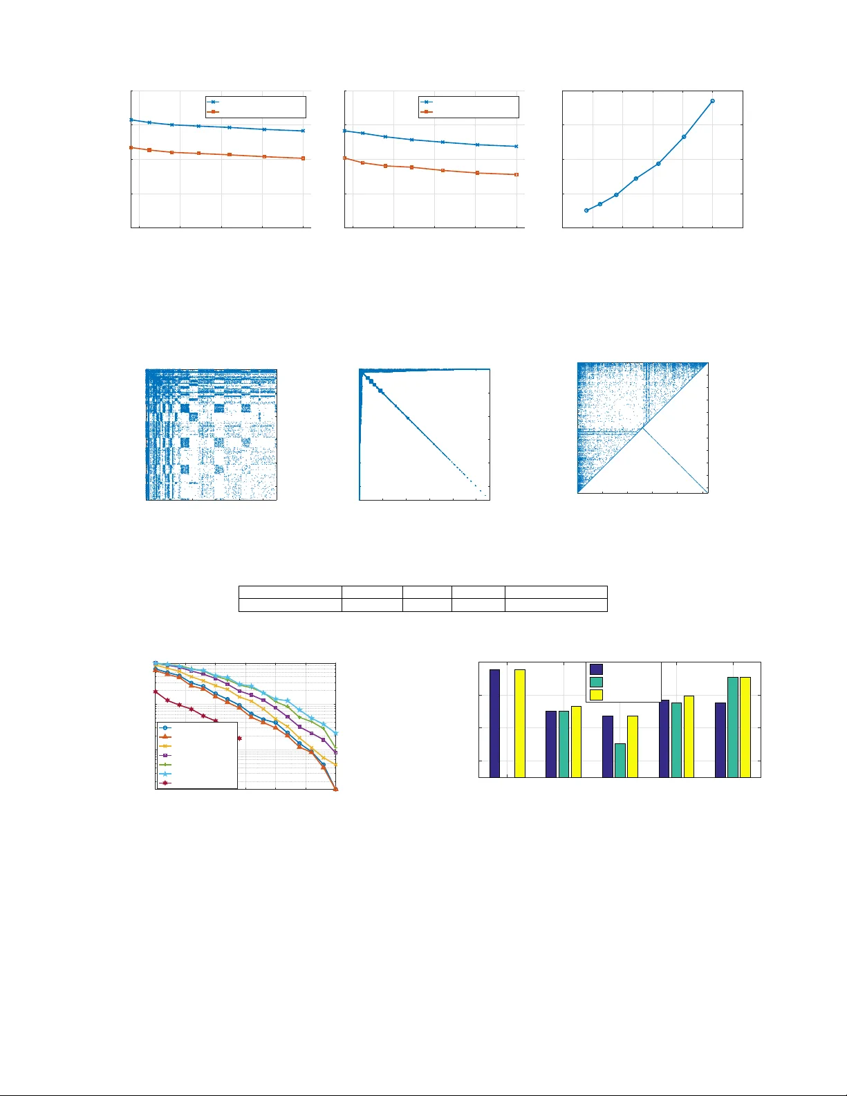
1 F ast P ath Localization on Graphs via Multiscale V iterbi Decoding Y aoqing Y ang ∗ † , Siheng Chen ∗ , Mohammad Ali Maddah-Ali † , Pulkit Grov er ∗ , Soummya Kar , ∗ and Jelena K ov a ˇ ce vi ´ c ∗ ∗ Carnegie Mellon Uni versity † Nokia Bell Labs Abstract —W e consider a pr oblem of localizing a path-signal that evolv es over time on a graph. A path-signal can be viewed as the trajectory of a moving agent on a graph in se veral consecutive time points. Combining dynamic programming and graph partitioning, we propose a path-localization algorithm with signiﬁcantly reduced computational complexity . W e analyze the localization error for the proposed approach both in the Ham- ming distance and the destination’ s distance between the path estimate and the true path using numerical bounds. Unlike usual theoretical bounds that only apply to restricted graph models, the obtained numerical bounds apply to all graphs and all non- overlapping graph-partitioning schemes. In random geometric graphs, we are able to derive a closed-form expression for the localization error bound, and a tradeoff between localization error and the computational complexity . Finally , we compare the proposed technique with the maximum likelihood estimate under the path constraint in terms of computational complexity and localization error , and show signiﬁcant speedup (100 × ) with comparable localization error (4 × ) on a graph from real data. V ariants of the proposed technique can be applied to tracking, road congestion monitoring, and brain signal pr ocessing. I . I N T RO D U C T I O N Data with unstructured forms and rich types are being generated from various sources, from social netw orks to biological netw orks, from citation graphs to kno wledge graphs, from the Internet of Things to urban mobility patterns. These data are often generated with some inherent dependencies that can be represented using graphs and thus inspired the emerging ﬁeld of graph signal processing [2], [3]. In graph signal processing, signals are supported on graphs, instead of on conv entional regular well-ordered domains (e.g., signals supported on the time grid or signals supported on other regular grids). This key difference spurred a lot of research that aims to generalize classical techniques to graph signal processing, including sampling [4]–[6], recov ery [7]–[9], sig- nal representations [10]–[12], uncertainty principles [13], [14], and graph signal transforms [15]–[19]. In this paper , we study a special type of dynamic signals on graphs that we call path-signals . A path-signal (see Fig. 1 for an illustration) is a special type of a graph signal that is supported on a connected trajectory , i.e., the signal is non- zero at only one location at each time point, and the non-zero locations at consecutiv e time points form a connected path on A preliminary v ersion of this work was presented in part at the IEEE Inter - national Conference on Acoustics, Speech and Signal Processing (ICASSP), 2017 [1]. This work is supported in part by the National Science Foundation under grants CCF-1513936, by ECCS-1343324 and CCF-1350314 (NSF CAREER) for Pulkit Grover , and by Systems on Nanoscale Information fabriCs (SONIC), one of the six SRC ST ARnet Centers, sponsored by MARCO and DARP A. t=1 t=2 t=T A A B B Fig. 1: A path-signal on a graph with ﬁv e nodes. The nodes with a non-zero signal v alue form a (connected) path on the graph (green dashed line). For example, the acti vated node at time t = 1 is v 1 = A and the activ ated node at time t = 2 is v 2 = B . For the signal to be a path-signal we require ( v 1 , v 2 ) ∈ E . A path-signal can be vie wed as an abstraction of the trajectory of a moving agent on a graph. the graph. A path-signal is an abstraction of a moving agent on a graph, where the non-zero location of the path-signal at a particular time point t can be viewed as the location of the moving agent on the graph at time t . Thus, the study of path-signals is deeply related to tracking and surveillance [20]. Here, we study the path-signals on large-scale graphs from the perspecti ve of graph partitioning and graph (signal) di- mension reduction: due to the increasing size of graphs, many techniques on dimension reduction for graphs or graph signals hav e been proposed, which include community detection and clustering on graphs [21]–[24] as well as signal coarsening on graphs [25]–[27]. These newly proposed techniques and related ideas have provided great improvements in compu- tation speed and storage cost for algorithms on large-scale graphs, including PageRank [28], graph generation [29] and graph semantic summarization [30]. By studying path-signals, we will be able to explore the connections between signal tracking and graph dimension reduction. In the path-signal problem, we consider two dif fer- ent subproblems: the “path-localization” problem and the “destination-localization” problem. The aim of the ﬁrst prob- lem is to estimate the trajectory of the moving agent, while the aim of the second problem is to estimate only the ﬁnal position of the moving agent, both from noisy observations of the path- signal. W e measure the accuracy of the ﬁrst problem using the metric of Hamming distance. For the second problem, we measure the path-localization accuracy using the Euclidean distance, assuming the graph is embedded in an Euclidean space (e.g., a geometric graph). First, we propose to use an algorithm based on dynamic programming to estimate the trajectory and destination of the path-signal on the original graph. This algorithm resembles the classical V iterbi decoding method in the context of conv olutional decoding [31]. W e also 2 show that this algorithm is the maximum likelihood (MLE) estimate under the path constraint. The computational comple xity of path MLE is high for lar ge graphs, which motiv ates us to design a f ast approximate algo- rithm. W e use graph partitioning techniques to di vide the graph into non-ov erlapping clusters and merge each cluster into a single “super-node”. Subsequently , we implement dynamic programming on the resulting graph deﬁned by these super- nodes. Since we track the path trajectory and path destination on the graph deﬁned by these clusters, we signiﬁcantly reduce the number of states in dynamic programming, and hence reduce the computation time. The proposed method can be viewed as implementing the V iterbi decoding method on a condensed graph and hence our approach is referred to as multiscale V iterbi decoding. Using large-de viation techniques, we provide bounds on the two distance measures (Hamming distance and the destination distance) respectiv ely for the path- localization problem and the destination-localization problem. W e show that both bounds can be computed in polynomial time for general graphs and general non-ov erlapping graph partitioning algorithms. Then, we focus on an important class of graphs, i.e., random geometric graphs with a simple square tessellation partition- ing. The random geometric graph is widely used for sensor networks [32], and thus is particularly relev ant for the study of tracking. In this case, we obtain a closed-form theoretical bound on the localization error . W e v alidate the multiscale V iterbi decoding algorithm on synthesized random geometric graphs by sho wing both theory and simulation results. Next, we consider real graph data coming from the au- tonomous systems in Oregon [33] and apply the multiscale V iterbi decoding algorithm with se veral well-kno wn graph par- titioning schemes. The graph partitioning scheme that achieves the best performance is the Slashburn algorithm [24], which is based on the idea that real networks have no good cuts (i.e., the vertices of the graph cannot be easily partitioned into two non-ov erlapping groups such that the number of edges that span the two groups is small) unless a small set of “hub- nodes” with high degree is remov ed. Our algorithm using graph partitioning shows signiﬁcant speedup and comparable localization performance with respect to the direct method that uses dynamic programming on the original graph without using graph partitioning. A closely related line of work considers the problem of detecting signals in irregular domains [34]–[39]. In particular , [40], [41] consider optimal random walk detection on a graph which is closely related to the problem of path localization. Howe ver , our problem setting considers path-signals that can be adversarial, in the sense that the proposed algorithm and theoretical bounds can be applied to worst-case path-signals. Moreov er , we consider approximate algorithms that have low computational complexity compared to the optimal localizers (such as the one based on MLE that is presented in Sec- tion II-C) but have comparable performance. The problem of path localization on graphs is strongly connected to signal tracking. If the graph is viewed as the state space and the Marko v transition probability is imposed by the graph topology , the path-localization problem is equiv alent to tracking. Howe ver , as we mentioned earlier , compared to tracking problems including Kalman ﬁltering [42] and particle ﬁltering [43], the proposed method applies to worst-case trajectory and signal. Some other related tracking problems include natural video tracking [44], cell tracking [45] and diffusion tensor imaging [46]. Those methods are often applied to regular signals such as time signals or images, but our paper considers signals supported on graphs. The proposed path-localization problem is related to track- ing and trajectory recovery in many different contexts, such as road congestion monitoring, satellite searching and brain signal processing [47]. A signal path on a road network can be viewed as a slowly moving congested segment on the graph formed by roads and intersections. A signal path in a satellite search can be viewed as the trajectory of a plane debris moved by ocean currents or the trajectory path of a small refugee lifeboat in the sea, while the observation noise may come from sensing inaccuracy and poor illumination conditions at night. The signal path in a brain imaging problem can be vie wed as consecutiv e ﬁring events of brain signals in the brain network. I I . S Y S T E M M O D E L A N D P RO B L E M F O R M U L A T I O N : P A T H - S I G NA L A N D P A T H L O C A L I Z A T I O N W e denote by G = ( V , E ) an undirected 1 graph with V as the set of nodes and E the set of edges, where |V | = n for some n ∈ Z + . W e use x t ∈ R n , t = 1 , 2 , . . . T to denote a deterministic (b ut unknown) time-series of (non-random) signals supported on the graph G = ( V , E ) that ev olve over time. The value x t ( v ) denotes the signal value at time t and at node v . Deﬁnition 1 . (Path-signal) A deterministic b ut unknown time- series of non-random signals x t ∈ R n , t = 1 , 2 , . . . T is called a path-signal on the graph G = ( V , E ) if at each time point t , there is one node v t such that x t ( v t ) = µ > 0 and x t ( v ) = 0 for all other nodes v 6 = v t . The collection of the nodes ( v 1 , v 2 , . . . v T ) forms a connected path , i.e., ( v t , v t +1 ) ∈ E for all t = 1 , 2 , . . . T − 1 . A path ( v 1 , v 2 , . . . v T ) can represent the trajectory of a moving agent on the graph G = ( V , E ) from time t = 1 to time t = T . W e call the sequence { x t } T t =1 the path-signal, since the signal value x t ( v ) on the path ( v 1 , v 2 , . . . v T ) has a shifted v alue µ > 0 . Let p ∗ = ( v ∗ 1 , v ∗ 2 , . . . v ∗ T ) be a connected path let { x t } T t =1 be a path signal. Let { y t } T t =1 be a sequence of noisy observations of a path-signal { x t } T t =1 where, y t = x t + w t , t = 1 , 2 , . . . T , (1) where w t ∼ N ( 0 , σ 2 I n × n ) is Gaussian noise. Our goal is to localize this connected path p ∗ = ( v ∗ 1 , v ∗ 2 , . . . v ∗ T ) on the graph G = ( V , E ) with shifted mean µ from the noisy observations { y t } T t =1 . W e will call p ∗ the “true path”. W e will use ˆ p = ( ˆ v 1 , ˆ v 2 , . . . ˆ v T ) to denote the chain estimate. 1 The proposed algorithms in this paper naturally apply to directed graphs as well. For the sake of consistency , we only consider undirected graphs in this paper . 3 A. T wo Err or Metrics for P ath Localization W e deﬁne two dif ferent error metrics on the path- localization problem. Using these two metrics, we can measure the inaccuracy of dif ferent path-localization algorithms. Deﬁnition 2 . (Hamming distance) The Hamming distance between the estimated chain ˆ p = ( ˆ v 1 , ˆ v 2 , . . . ˆ v T ) and the true path p ∗ = ( v ∗ 1 , v ∗ 2 , . . . v ∗ T ) is deﬁned as D H ( ˆ p , p ∗ ) = T X t =1 1 ( ˆ v t 6 = v ∗ t ) , (2) where 1 ( · ) denotes the indicator function. Deﬁnition 3 . (Destination distance) The destination distance D F ( ˆ p , p ∗ ) between the estimated chain ˆ p = ( ˆ v 1 , ˆ v 2 , . . . ˆ v T ) and the true path p ∗ = ( v ∗ 1 , v ∗ 2 , . . . v ∗ T ) is deﬁned as D F ( ˆ p , p ∗ ) = d ( ˆ v T , v ∗ T ) , (3) where the distance d ( ˆ v T , v ∗ T ) is a distance metric between the two nodes ˆ v T and v ∗ T deﬁned for the graph G (which can either be the multi-hop distance 2 on a general graph or the Euclidean distance on a geometric graph [48] embedded in an Eclidean space). The Hamming distance measures the inaccurac y of the chain estimate by counting the overall number of mismatched nodes, while the destination distance directly measures the distance between the ﬁnal positions of the chain estimate and the true path. The second metric is more useful when the goal is to make an estimate of the current position of the moving agent. W e also call the path estimation problem with the destination distance metric the destination-localization problem. Here, we only consider localizing each position v ∗ t giv en the entire signal { y t } T t =1 . A generalized problem is that we want to localize each position v ∗ t using only the observ ations up to time t , i.e., { y τ } t τ =1 . B. Constrained Maximum Likelihood Chain Estimators Denote by V T the T -fold Cartesian product of the node set V . Note that V T is the set of all possible chains of nodes of length T . Deﬁnition 4 . ( S -constrained MLE) For an arbitrary set S ⊂ V T , deﬁne the S -constrained maximum likelihood estimate (MLE) ˆ p MLE S as the chain in S that has the maximum like- lihood value for the observed signal y t , t = 1 , . . . T . That is p MLE S = arg max ˆ p ∈S Pr (( y 1 , . . . , y T ) | p ∗ = ˆ p ) . (4) First, we show that the S -constrained MLE has the maxi- mum sum signal over all chains in S . For an arbitrary chain of nodes ˆ p = ( ˆ v 1 , ˆ v 2 , . . . ˆ v T ) ∈ S , we deﬁne the sum signal S ( ˆ p ) = T X t =1 y t ( ˆ v t ) . (5) 2 The multi-hop distance between two nodes on an undirected graph is the minimum number of hops required to reach one node from the other through a chain of edges. Intuitiv ely , a chain with a higher sum signal 3 is more likely to be the true path p ∗ . In fact, it coincides with the S -constrained MLE, as sho wn below: Pr (( y 1 , . . . , y T ) | p ∗ ) = T Y t =1 C exp  − 1 2 σ 2 k y t − x t k 2 2  = C T exp − 1 2 σ 2 T X t =1 k y t − x t k 2 2 ! , where recall that p ∗ = ( v ∗ 1 , v ∗ 2 , . . . v ∗ T ) denotes the true path and C is a constant. Then, arg max ˆ p ∈S Pr (( y 1 , . . . , y T ) | p ∗ = ˆ p ∈ S ) = arg min ˆ p ∈S T X t =1 k y t − x t k 2 2 = arg max ˆ p ∈S T X t =1 y t · x t = arg max ˆ p ∈S T X t =1 µ y t ( v t ) = arg max ˆ p =( ˆ v 1 , ˆ v 2 ,... ˆ v T ) ∈S T X t =1 y t ( ˆ v t ) . (6) Then, we consider two extreme cases of S -constrained MLE. In the ﬁrst case, we set S = V T . In this case, the S - constrained MLE is a nai ve estimator that completely ignores the path constraint. In fact, since the signals on each time point is independent of each other, the S -constrained MLE is ˆ p MLE V T = ( ˆ v 1 , ˆ v 2 , . . . ˆ v T ) , where ˆ v t = arg max ˆ v ∈V y t ( ˆ v ) , t = 1 , 2 , . . . , T . (7) Although this estimator is extremely simple, it does not perform well respect to the proposed distance metrics in Deﬁnition 2 and 3 due to ignoring the path constraint (we will sho w this later in Section V). The second S -constrained MLE is the maximum likeli- hood estimator under the constraint that the estimator ˆ p = ( ˆ v 1 , ˆ v 2 , . . . ˆ v T ) has to be a path. W e describe this particular S -constrained MLE in the following section. C. P ath-constrained MLE using V iterbi Decoding From (6), if we impose the constraint that ˆ p must be a connected path, the MLE estimate of p ∗ is the connected path with the maximum sum signal. In Algorithm 1, we describe a dynamic programming algorithm to compute a connected path with the maximum sum signal. This algorithm is also known as the V iterbi decoding algorithm in the context of con volutional decoding [31]. The basic idea in Algorithm 1 is to record the path with the largest sum signal of length t that ends at node v for all nodes in the graph G and all time points t = 1 , 2 , . . . T . Although the possible number of paths is exponential in t , Algorithm 1 has computational complexity O ( nT ) , because only the optimal path, instead of all paths, that ends at a node v has to be recorded at each time t . 3 Note that we want to localize the position v t of the path at each particular time point t = 1 , 2 , . . . T , instead of all positions that the path has passed through aggregated in a single snapshot. For the problem of aggregating all locations that the path has passed through in a single snapshot, we may simply compute the sum of all signals P T t =1 y t in all time points and select the nodes v with a higher sum signal. 4 Algorithm 1 Dynamic Programming for Path-Signal Local- ization INPUT : A graph G = ( V , E ) and graph signal observ ations y t , t = 1 , 2 , . . . T . OUTPUT : A chain of nodes ˆ p = ( ˆ v 1 , ˆ v 2 , . . . ˆ v T ) . INITIALIZE Use s v ,t to denote the sum signal until time t at node v . Use p v ,t to denote the path with the largest sum signal of length t that ends at node v . Initialize p v , 1 = v for all v ∈ V . FOR t = 2 : T • For all nodes v in V , let u m = arg max u ∈N ( v ) S ( p u,t − 1 ) , where N ( v ) denotes the neighborhood of v . Therefore, the path p u m ,t − 1 has the largest sum signal S ( p u,t − 1 ) for all nodes u in the neighborhood N ( v ) ; • Update p v ,t = ( p u m ,t − 1 , v ) for all v ∈ V . END Denote by p v ∗ ,T the path with the largest sum signal in all paths of length T . Output ˆ p = p v ∗ ,T . The S -constrained MLE with S being all connected paths in V T has much better empirical performance than the naive maximization ˆ p MLE V T in (7) (we will sho w this later in Sec- tion V). Howe ver , the computational complexity O ( nT ) is high for a large graph and a large ov erall time T . This motiv ates us to design some approximate algorithms that hav e low computational complexity (see Section III). Remark 1 . Note that in the path-localization problem, we do not require the estimated chain of nodes ˆ p = ( ˆ v 1 , ˆ v 2 , . . . ˆ v T ) to be connected, i.e., ( ˆ v t , ˆ v t +1 ) ∈ E , t = 1 , 2 , . . . T − 1 . As long as we hav e an estimated chain of nodes with small Hamming distance or destination distance as deﬁned in Deﬁnition 2 and 3, the estimate is good. The naiv e V T -constrained MLE in (7) is bad, not because it is disconnected, but because it totally ignores the path constraint and results in large Hamming distance. The path-constrained MLE is good in empirical performance b ut it has high computational complexity . T o resolve this issue, we propose an approximate path estimate in Section III, which is not necessarily connected in the original graph G , but connected in a graph formed by subgraphs (we will present the details in SectionII-C). Moreov er , it has lower computational complexity (100+ times speed-up) than the path-constrained MLE, and comparable localization error (4 × in Hamming distance). Therefore, the approximate path estimate can be viewed as a relaxed version of path- constrained MLE, with lo wer computational complexity . I I I . M U LT I S C A L E V I T E R B I D E C O D I N G F O R F A S T P A T H - S I G N A L L O C A L I Z A T I O N In this section, we design an algorithm that combines path localization with graph partitioning. As we have mentioned in Section II, we want to use an estimation technique that has very low computational complexity . Our main idea is to ﬁrst partition the original graph into clusters [49] and localize an Cluster 1 Cluster 2 Cluster 3 Cluster 4 A graph formed by clusters Super-node 1 Super-node 2 Super-node 3 Super-node 4 Fig. 2: An illustration of the graph formed by clusters. In the original graph G , we partition the nodes into non-ov erlapping clusters. Then, we shrink each cluster to one “super-node” and connect two super-nodes if there exist two connected nodes in the corresponding two clusters. The “super-graph” may hav e self-loops but our algorithms still apply . approximate path on a new graph formed by the clusters 4 . Then, we do a reﬁned search inside the approximate path to search for a chain of nodes that well approximates the true path in the original graph in terms of the Hamming distance and the destination distance. Suppose we partition the nodes of the graph G = ( V , E ) into m non-ov erlapping clusters V = m [ i =1 V i . (8) Then, we shrink each cluster into a “super-node” and construct a new graph denoted by G new = ( V new , E new ) formed by these super-nodes as follows. The node set V new with cardinality |V new | = m is the set of “super-nodes”. T wo nodes V i and V j are connected if there exists two nodes v i ∈ V i and v j ∈ V j such that ( v i , v j ) ∈ E in the original graph G . W e call the graph G new the super-graph (see Fig. 2). Consider the observ ation model described in (1) on a general graph G = ( V , E ) such that x t ( v t ) = µ and x t ( v ) = 0 for v 6 = v t , and ( v 1 , v 2 , . . . v T ) is a connected path in G . Suppose we use a graph-partitioning algorithm and obtain the super-graph G new = ( V new , E new ) . W e use a coarsened [25]–[27] version u t of the original observation y t as the graph signal on the super-graph. The coarsened graph signal is deﬁned as u t ( V i ) = max v ∈V i y t ( v ) , i = 1 , 2 , . . . m. (9) W e will brieﬂy discuss the reason that we choose the max statistic instead of other statistics such as average in Remark 2. Then, using the coarsened signal, we execute the same dy- namic programming algorithm as Algorithm 1 to obtain an estimate of the trajectory of the path-signal on the super-graph (see Algorithm 2). Note that after graph partitioning, the sum signal maximization does not equal to the MLE because the signal u t ( V i ) ’ s are not Gaussian. Howe ver , we will sho w an upper bound on the e xpectation of the Hamming and destina- tion distance between the true path and the path estimate on the super-graph G new (see Section III-A). Therefore, Algorithm 2 4 The graph partitioning that we consider only means the partitioning of the node set V into non-overlapping subsets. It does not necessarily correspond to the usual deﬁnition of graph partitioning, i.e., the number of intra-cluster edges is greater than number of inter-cluster edges and the number of nodes in different clusters should be similar . 5 Algorithm 2 Coarsened Dynamic Programming for Path- Signal Localization INPUT : A coarsened graph G new = ( V new , E new ) and coars- ened graph signal observ ations u t , t = 1 , 2 , . . . T . OUTPUT : A chain of nodes ˆ P = ( ˆ V 1 , ˆ V 2 , . . . ˆ V T ) on the super-graph. Call Algorithm 1 with inputs G new = ( V new , E new ) and u t , t = 1 , 2 , . . . T . is an approximate path localization algorithm that aims to reduce computational complexity of MLE. Remark 2 . Choosing the max statistic instead of the mean statistic is reminiscent of the generalized likelihood ratio test (GLR T) [50] for composite hypothesis testing. Although our idea of choosing the max statistic is inﬂuenced by GLR T , our localization algorithm is not GLR T . Another reason that we choose the max statistic instead of the mean statistic for approximate path localization is that the max statistic has a better localization error than the mean statistic. Consider a cluster V with one activ ated node v 0 . The mean statistic is u mean = 1 |V | P v ∈V y t ( v ) and the max statistic is u max = max v ∈V y t ( v ) . When the number of nodes |V | → ∞ , u mean → 0 almost surely , while u max = max v ∈V y t ( v ) still provides some information about the acti vated node. For a ﬁnite |V | , as long as the noise v ariance is small, the max statistic can cancel the noise sufﬁciently well and giv e a coarsened signal that equals y t ( v 0 ) , the signal at the acti vated node v 0 . Ho wev er , if we choose the mean statistic u mean = 1 |V | P v ∈V y t ( v ) , y t ( v 0 ) is always averaged by noise, which makes the performance of the multiscale V iterbi Decoding algorithm degrade. The analysis of the max statistic is established later formally using large-deviation bounds in Section III-A. Note that our algorithm and the bounds in Section III-A apply to worst-case path-signals and graph partitioning, which is dif ferent from the Bayesian settings in [40], [41]. After ex ecuting Algorithm 2, we obtain an approximate path estimate ˆ P = ( ˆ V 1 , ˆ V 2 , . . . ˆ V T ) in the super-graph. In some tracking and surveillance applications, an approximate path estimate is good enough for subsequent actions. Howe ver , in most cases we want to obtain an estimate not only in the super-graph, but also in the original graph, especially when the clusters are large and the exact positions of the agent are required. In this case, we do a reﬁned search in the original graph in the path ˆ P = ( ˆ V 1 , ˆ V 2 , . . . ˆ V T ) that we obtained in the super-graph. Therefore, we propose the ﬁnal multiscale V iterbi decoding method in Algorithm 3. In Supplementary Section VII, we extend the Multiscale V iderbi decoding algorithm to the situation when we hav e more than one path. Remark 3 . As we can see from Algorithm 3, although the path estimate ˆ P = ( ˆ V 1 , ˆ V 2 , . . . ˆ V T ) is a connected path in the super - graph, the chain estimate ˆ p is not necessarily a connected path in the original graph because we choose the node ˆ v t with the largest signal in ˆ V t without a path constraint. Howe ver , as we mentioned in Remark 1, as long as the distance metric between the estimated chain ˆ p and the true path is small, it does not Algorithm 3 Multiscale V iterbi Decoding for Path Localiza- tion INPUT : A graph G = ( V , E ) and graph signal observ ations y t , t = 1 , 2 , . . . T . OUTPUT : A chain of nodes ˆ p = ( ˆ v 1 , ˆ v 2 , . . . ˆ v T ) . INITIALIZE Call Algorithm 2 with inputs G = ( V , E ) and y t , t = 1 , 2 , . . . T to obtain a coarse path estimate ˆ P = ( ˆ V 1 , ˆ V 2 , . . . ˆ V T ) . Choose ˆ v t as the node that has the largest signal in ˆ V t , i.e., ˆ v t = arg max v ∈ ˆ V t y t ( v ) . Let ˆ p = ( ˆ v 1 , ˆ v 2 , . . . ˆ v T ) be the ﬁnal chain estimate in the original graph. matter whether ˆ p is connected or not. Therefore, ˆ p can be viewed as an estimate when the path constraint is relaxed. Deﬁne P ∗ = ( V ∗ 1 , V ∗ 2 , . . . V ∗ T ) as the true path in the super-graph, i.e., the true path in the original graph p ∗ = ( v ∗ 1 , v ∗ 2 , . . . v ∗ T ) satisﬁes v ∗ t ∈ V ∗ t , ∀ t . Note that the Ham- ming distance between the approximate path estimate ˆ P = ( ˆ V 1 , ˆ V 2 , . . . ˆ V T ) (output from Algorithm 2) and the true path P ∗ in the super-graph is alw ays a lower bound on the Ham- ming distance between the chain estimate ˆ p = ( ˆ v 1 , ˆ v 2 , . . . ˆ v T ) (output from Algorithm 3) and the true path p ∗ in the original graph, i.e., D H ( ˆ P , P ∗ ) ≤ D H ( ˆ p , p ∗ ) . (10) This is because ˆ p is constrained inside the approximate path ˆ P , and hence ˆ V t 6 = V ∗ t implies ˆ v t 6 = v t . Howe ver , in Section V, we use a simulation result on a real graph (see Fig. 6 for details) to sho w that D H ( ˆ p , p ∗ ) is only slightly larger than D H ( ˆ P , P ∗ ) . This means that e ven if we impose the connected path constraint when doing the reﬁned search and use other techniques such as a second round of dynamic programming in the subgraph induced from the path estimate obtained from Algorithm 2 to obtain a connected path in the original graph, we cannot gain too much compared to simply choosing the node with the maximum signal in each cluster as we do in Algorithm 3. In the ne xt section, we show a numeric way to compute an upper bound on both the Hamming distance and destination distance in Algorithm 2 and Algorithm 3 in polynomial time (more speciﬁcally , linear in the number of clusters m and at most quadratic in the total number of time points T ). A. A Numeric Method for Computing an Upper Bound on the Localization Err or First, we introduce some notation for the analysis of the localization error of the multiscale V iterbi decoding algorithm. W e use W off to denote a Gaussian random v ariable N ( 0 , σ 2 ) and use U on to denote a Gaussian random v ariable N ( µ, σ 2 ) . W e use the superscripts “on” and “of f ” because the signal on the path has an elev ated mean value µ while the signal off the path has mean value 0. W e use W off s to denote a random variable that is the maximum of s i.i.d. Gaussian random variables with the same distribution as W off ∼ N ( 0 , σ 2 ) . W e use U on s to denote a random v ariable that is the maximum of one Gaussian random variable with the same distribution 6 as U on ∼ N ( µ, σ 2 ) and s − 1 Gaussian random v ariables W off ∼ N ( 0 , σ 2 ) . Recall that P ∗ = ( V ∗ 1 , V ∗ 2 , . . . V ∗ T ) is the true path in the super-graph and ˆ P = ( ˆ V 1 , ˆ V 2 , . . . ˆ V T ) is the path estimate in the super-graph. Note that at some positions, the two paths may overlap, i.e., ˆ V t = V ∗ t for some t . Denote by S ( P ∗ ) the sum signal of the true path P ∗ in the super-graph, and denote by S ( ˆ P ) the sum signal on the path estimate ˆ P in the super- graph. Then, from (9), Sum signal on the true path P ∗ : S ( P ∗ ) = T X t =1 u t ( V ∗ t ) , (11) Sum signal on the path estimate ˆ P : S ( ˆ P ) = T X t =1 u t ( ˆ V t ) , (12) where on the true path, u t ( V ∗ t ) D = U on |V ∗ t | and on the path estimate, if ˆ V t 6 = V ∗ t , u t ( ˆ V t ) D = W off | ˆ V t | ( D = means equal in distribution). Here recall that U on s denotes the maximum of one Gaussian random variable with mean µ and s − 1 Gaussian random variables with mean 0 , W off s denotes the maximum of s Gaussian random v ariables with mean 0 , and |V ∗ t | and | ˆ V t | denote respectively the number of nodes in the cluster that the true path passes through at time t , and the path estimate passes through at time t . In the dynamic programming Algorithm 2 in the super-graph, we will select the path with the maximum sum signal. Therefore, we will choose the path estimate ˆ P with sum signal S ( ˆ P ) instead of the true path P ∗ with sum signal S ( P ∗ ) , only if S ( ˆ P ) ≥ S ( P ∗ ) . This ev ent happens with exponentially low probability because the signal on the true path has a shifted mean value µ > 0 , while the signal on ˆ P has mean v alue 0 when the two paths do not ov erlap. Lemma 1 . The probability that the sum signal S ( ˆ P ) of the path estimate ˆ P = ( ˆ V 1 , ˆ V 2 , . . . ˆ V T ) is greater or equal to the sum signal S ( P ∗ ) on the true path P ∗ = ( V ∗ 1 , V ∗ 2 , . . . V ∗ T ) can be upper bounded by Pr( S ( ˆ P ) ≥ S ( P ∗ )) ≤ Y t ∈ ∆ θ  µ 2 σ 2 , | ˆ V t |  , (13) where ∆ ⊂ { 1 , 2 , . . . T } is the set of time indices at which ˆ V t 6 = V ∗ t , and the function θ ( · , · ) is deﬁned as θ ( s, l ) := min η ∈ [0 , 1] lη l − 1 e s 2 σ 2 − µs Q ( Q − 1 ( η /σ ) − sσ 2 ) + r l 2 2 l − 1 (1 − η 2 l − 1 ) e 3 2 s 2 σ 2 − µs p Q ( Q − 1 ( η /σ ) − 2 sσ 2 ) , (14) where s ∈ R and l ∈ Z + . Pr oof: See Supplementary Section VI for details of the proof. The basic idea of the proof is to use large-de viation techniques to bound the event S ( ˆ P ) ≥ S ( P ∗ ) , which is equiv alently to T X t =1 u t ( V ∗ t ) ≤ T X t =1 u t ( ˆ V t ) , (15) where u t ( V ∗ t ) is the coarsened signal on the true approximate path P ∗ at time t and u t ( ˆ V t ) is the coarsened signal on ˆ P at time t . Both u t ( V ∗ t ) and u t ( ˆ V t ) are maximum of certain Gaussian random variables, but u t ( V ∗ t ) has one Gaussian random v ariable with an elev ated mean value µ , and hence is more likely to be lar ger than u t ( ˆ V t ) . More speciﬁcally , using the large-de viation bound and some deriv ations, we obtain Pr( S ( ˆ P ) ≥ S ( P ∗ )) ≤ min s> 0 Y t ∈ ∆ E h e s u t ( ˆ V t ) i E h e − s u t ( V ∗ t ) i . (16) The bound in (13) is obtained by directly upper -bounding the right hand side of (16). Using the conclusion of Lemma 1, we immediately obtain the follo wing results respecti vely regarding the localization error metrics in Deﬁnition 2 and Deﬁnition 3. The proofs are omitted because they are direct applications of the follo wing union bound E h D ( P ∗ , ˆ P ) i = X ∀ ˆ P Pr( ˆ P is the chosen estimate ) D ( P ∗ , ˆ P ) , (17) where P ∀ ˆ P is summation ov er all possible paths ˆ P = ( ˆ V 1 , ˆ V 2 , . . . ˆ V T ) in the super-graph, D ( · , · ) can be either the Hamming distance D H ( · , · ) or the destination distance D F ( · , · ) . Theor em 1 . (Hamming distance in Algorithm 2) The expecta- tion of the Hamming distance between the path estimate and the true path measured on the super-graph is upper bounded by E h D H ( P ∗ , ˆ P ) i ≤ X ∀ ˆ P   | ∆( ˆ P ) | Y t ∈ ∆( ˆ P ) θ  µ 2 σ 2 , | ˆ V t |    ≤ min δ ∈ [0 , 1] δ T + X ∀ ˆ P s.t. | ∆( ˆ P ) | >δT   | ∆( ˆ P ) | Y t ∈ ∆( ˆ P ) θ  µ 2 σ 2 , | ˆ V t |    , (18) where ∆( ˆ P ) denotes the set of time indices at which the path estimate ˆ V t is wrong, i.e., ∆( ˆ P ) = { t ∈ { 1 , 2 , . . . T } : ˆ V t 6 = V ∗ t } , (19) and θ ( · , · ) is deﬁned in (14). Theor em 2 . (Destination distance in Algorithm 2) The expec- tation of the destination distance between the path estimate and the true path measured on the super-graph is upper bounded by E h D F ( P ∗ , ˆ P ) i ≤ X ∀ ˆ P   d ( V ∗ T , ˆ V T ) Y t ∈ ∆( ˆ P ) θ  µ 2 σ 2 , | ˆ V t |    , (20) where ∆( ˆ P ) ⊂ { 1 , 2 , . . . T } is the set of time indices t at which ˆ V t 6 = V ∗ t , θ ( · , · ) is deﬁned in (14), and d ( V ∗ T , ˆ V T ) is the distance metric between the two super-nodes V ∗ T and ˆ V T in the super-graph. The proofs for these two bounds are omitted because they follow directly from (17). The second inequality in (18) is obtained by only counting the paths that satisfy | ∆( ˆ P ) | > δ T . The two bounds in Theorem 1 and Theorem 2 are stated for the distance metric stated in the super-graph. Howe ver , for Algorithm 3, we have to compute the distance metric in the original graph. Likewise, we will select a path with the 7 maximum sum signal in Algorithm 3, so we can upper-bound the probability of choosing a particular path using an event that happens with small probability . Deﬁnition 5 . W e will call P = ( V 1 , V 2 , . . . V T ) in the super - graph G new = ( V new , E new ) the pr ojected path of a path p = ( v 1 , v 2 , . . . v T ) in the original graph G = ( V , E ) if v t ∈ V t for t = 1 , 2 , . . . T . For the true path P ∗ = ( V ∗ 1 , V ∗ 2 , . . . V ∗ T ) , deﬁne the “ﬁrst- k ” sum as f ( k ) = max { t 1 ,t 2 ,...t k }⊂ [ T ] k X i =1 θ  µ 2 σ 2 , |V ∗ t |  , (21) where θ ( · , · ) is deﬁned in (14). Theor em 3 . (Hamming distance in Algorithm 3) Let ˆ p be the estimated chain of nodes using Algorithm 3 and let p ∗ be the true path. Let P ∗ be the projected path of p ∗ . The expectation of the Hamming distance between ˆ p and the true path p ∗ measured in the original graph is upper bounded by E [ D H ( p ∗ , ˆ p )] ≤ min δ ∈ [0 , 1] δ T + X ∀ ˆ P s.t. | ∆( ˆ P ) | >δT   | ∆( ˆ P ) | Y t ∈ ∆( ˆ P ) θ  µ 2 σ 2 , | ˆ V t |    + X ∀ ˆ P f ( T − | ∆( ˆ P ) | ) Y t ∈ ∆( ˆ P ) θ  µ 2 σ 2 , | ˆ V t |  , (22) where ∀ ˆ P means all possible paths ˆ P = ( ˆ V 1 , ˆ V 2 , . . . ˆ V T ) in the super -graph, ∆( ˆ P ) ⊂ { 1 , 2 , . . . T } is the set of time indices t at which ˆ V t 6 = V ∗ t , and θ ( · , · ) is deﬁned in (14). Pr oof: W e partition all possible paths ˆ p = ( ˆ v 1 , . . . ˆ v T ) into groups, so that all paths in the group M ˆ P hav e the same projected path ˆ P in the super-graph. Since there are m clusters in total, we ha ve at most m T groups. For each coarse path ˆ P = ( ˆ V 1 , . . . ˆ V T ) , denote by ∆( ˆ P ) ⊂ { 1 , 2 , . . . T } the set of time indices t at which ˆ V t 6 = V ∗ t . For each path ˆ p = ( ˆ v 1 , . . . ˆ v T ) , denote by L ( ˆ p ) ⊂ { 1 , 2 , . . . T } the set of time indices t at which ˆ v t 6 = v ∗ t . Now for each group M ˆ P , if one path in this group is chosen as the ﬁnal path estimate ˆ p , two things must happen. The ﬁrst is that the sum signal on the projected path ˆ P is larger than the sum signal on the true projected path P ∗ , because only in this way can we choose ˆ P as the coarse path estimate when calling Algorithm 2 in the INITIALIZE step of the multiscale V iterbi decoding Algorithm 3. This e vent is equi valent to X t ∈ ∆( ˆ P ) u t ( ˆ V t ) ≥ X t ∈ ∆( ˆ P ) u t ( V ∗ t ) . (23) The second thing that must happen is that ˆ p is just the set of nodes that achie ves the maximum signals in ˆ P = ( ˆ V 1 , ˆ V 2 . . . ˆ V T ) . In particular, for t ∈ L ( ˆ p ) \ ∆( ˆ P ) , which is the set of time indices at which the coarse path estimate ˆ P and the true coarse path P ∗ ov erlap but the path estimate ˆ p and the true path p ∗ differ , we must hav e y t ( ˆ v t ) ≥ y t ( v ∗ t ) , ∀ t ∈ L ( ˆ p ) \ ∆( ˆ P ) (24) These two ev ents are independent of each other, because the set of time points that they inv olve do not ov erlap, and all observations in different time points are independent of each other . Deﬁne W t = u t ( ˆ V t ) and U t = u t ( V ∗ t ) . Deﬁne β t = y t ( ˆ v t ) and α t = y t ( v ∗ t ) . The Hamming distance between the path estimate ˆ p and the true path p ∗ is the cardinality of the set L ( ˆ p ) , which is equal to the summation | L ( ˆ p ) \ ∆( ˆ P ) | + | ∆( ˆ P ) | . Using the union bound, the expectation of the ov erall Hamming distance between the path estimate ˆ p and the true path p ∗ can thus be upper-bounded by E [ D H ( p ∗ , ˆ p )] = E [ | ∆( ˆ P ) | ] + E [ | L ( ˆ p ) \ ∆( ˆ P ) | ] . (25) Now we look at the ﬁrst part. Using the union bound E [ | ∆( ˆ P ) | ] ≤ X ∀ ˆ P | ∆( ˆ P ) | Pr   X t ∈ ∆( ˆ P ) u t ( ˆ V t ) ≥ X t ∈ ∆( ˆ P ) u t ( V ∗ t )   . (26) First, we upper-bound the term p 1 := Pr  P t ∈ ∆( ˆ P ) u t ( ˆ V t ) ≥ P t ∈ ∆( ˆ P ) u t ( V ∗ t )  . Notice that the e vent P t ∈ ∆( ˆ P ) u t ( ˆ V t ) ≥ P t ∈ ∆( ˆ P ) u t ( V ∗ t ) is the same as the e vent P T t =1 u t ( V ∗ t ) ≤ P T t =1 u t ( ˆ V t ) , because ∆( ˆ P ) is the set of time indices t at which V ∗ t 6 = ˆ V t . This is just the e vent that the sum signal on ˆ P is greater that on P ∗ . By Lemma 1, p 1 ≤ Y t ∈ ∆ θ  µ 2 σ 2 , | ˆ V t |  , (27) where θ ( · , · ) is deﬁned in (14). Therefore, E [ | ∆( ˆ P ) | ] ≤ X ∀ ˆ P | ∆( ˆ P ) | Y t ∈ ∆( ˆ P ) θ  µ 2 σ 2 , | ˆ V t |  . (28) If we only compute the sum over the paths such that | ∆( ˆ P ) | > δ T , we can upper bound the expected Hamming distances of other paths by δ T . Therefore, E [ | ∆( ˆ P ) | ] ≤ δ T + X ∀ ˆ P s.t. | ∆( ˆ P ) | >δT | ∆( ˆ P ) | Y t ∈ ∆( ˆ P ) θ  µ 2 σ 2 , | ˆ V t |  . (29) For the second term E [ | L ( ˆ p ) \ ∆( ˆ P ) | ] , we use the union bound for all paths in M ˆ P , i.e., for all paths whose projected path is ˆ P . Using the union bound, we have E [ | L ( ˆ p ) \ ∆( ˆ P ) | ] ≤ X ∀ ˆ P Pr   X t ∈ ∆( ˆ P ) u t ( ˆ V t ) ≥ X t ∈ ∆( ˆ P ) u t ( V ∗ t )   · X ˆ p ∈M ˆ P | L ( ˆ p ) \ ∆( ˆ P ) | Y t ∈ L \ S Pr( ˆ v t 6 = v ∗ t ) Y t ∈ L c Pr( ˆ v t = v ∗ t ) , (30) where the Q t ∈ L \ S Pr( ˆ v t 6 = v ∗ t ) Q t ∈ L c Pr( ˆ v t = v ∗ t ) factor represents the probability that for t ∈ L ( ˆ p ) \ ∆( ˆ P ) , the coarse path estimate ˆ P and the true coarse path P ∗ ov erlap but the path estimate ˆ p and the true path p ∗ differ . Now look at the second line of the abov e inequality . For a ﬁxed path ˆ p with a ﬁxed projected path estimate ˆ P , | L ( ˆ p ) \ ∆( ˆ P ) | = X τ ∈ [ T ] \ ∆( ˆ P ) 1 ( ˆ v τ 6 = v ∗ τ ) . (31) 8 By changing the order of summation, X ˆ p ∈M ˆ P | L ( ˆ p ) \ ∆( ˆ P ) | Y t ∈ L \ S Pr( ˆ v t 6 = v ∗ t ) Y t ∈ L c Pr( ˆ v t = v ∗ t ) = X ˆ p ∈M ˆ P X τ ∈ [ T ] \ ∆( ˆ P ) 1 ( ˆ v τ 6 = v ∗ τ ) Y t ∈ L \ S Pr( ˆ v t 6 = v ∗ t ) Y t ∈ L c Pr( ˆ v t = v ∗ t ) = X τ ∈ [ T ] \ ∆( ˆ P ) X ˆ p ∈M ˆ P 1 ( ˆ v τ 6 = v ∗ τ ) Y t ∈ L \ S Pr( ˆ v t 6 = v ∗ t ) Y t ∈ L c Pr( ˆ v t = v ∗ t ) = X τ ∈ [ T ] \ ∆( ˆ P ) X ˆ p ∈M ˆ P s.t. ˆ v τ 6 = v ∗ τ Y t ∈ L \ S Pr( ˆ v t 6 = v ∗ t ) Y t ∈ L c Pr( ˆ v t = v ∗ t ) . (32) In the last summation, we sum up the binomial terms for all paths that satisfy ˆ v τ 6 = v ∗ τ , so the ﬁnal result will only be Pr( ˆ v τ 6 = v ∗ τ ) . Therefore, X ˆ p ∈M ˆ P | L ( ˆ p ) \ ∆( ˆ P ) | Y t ∈ L \ S Pr( ˆ v t 6 = v ∗ t ) Y t ∈ L c Pr( ˆ v t = v ∗ t ) = X τ ∈ [ T ] \ ∆( ˆ P ) Pr( ˆ v τ 6 = v ∗ τ ) = X t ∈ [ T ] \ ∆( ˆ P ) Pr( y t ( ˆ v t ) ≥ y t ( v ∗ t )) . (33) The last equality is because from the earlier discussion, for the time t ∈ [ T ] \ ∆( ˆ P ) (when the coarse projected path ˆ P overlaps with the true path P ∗ ), the estimate ˆ v t 6 = v ∗ t if and only if y t ( ˆ v t ) ≥ y t ( v ∗ t ) . Then, we upper-bound the term p 2 := Pr( y t ( ˆ v t ) ≥ y t ( v ∗ t )) = Pr( β t ≥ α t ) . Using the Marko v inequality , for all γ > 0 , p 2 = Pr (exp ( γ ( β t − α t )) ≥ 1) ≤ min γ > 0 E [exp ( γ ( β t − α t ))] = min γ > 0 E h e γ β t i E  e − γ α t  . (34) From the deﬁnitions of β t , we kno w for t ∈ L ( ˆ p ) \ ∆( ˆ P ) , the estimated path ˆ P and the true path P ∗ ov erlap, i.e., ˆ V t = V ∗ t . This means β t is the maximum of | ˆ V t | − 1 = |V ∗ t | − 1 i.i.d. random variables W off i , where each W off i D = W off ∼ N (0 , σ 2 ) . From the deﬁnition of α t , α t has the same distribution as U on ∼ N ( µ, σ 2 ) . Therefore, using the same large-de viation bounding techniques from the proof of Lemma 1 (see (61) to (64) for details), we hav e p 2 ≤ θ  µ 2 σ 2 , |V ∗ t |  . (35) Finally E [ | L ( ˆ p ) \ ∆( ˆ P ) | ] ≤ X ∀ ˆ P Pr   X t ∈ ∆( ˆ P ) u t ( ˆ V t ) ≥ X t ∈ ∆( ˆ P ) u t ( V ∗ t )   X ˆ p ∈M ˆ P | L ( ˆ p ) \ ∆( ˆ P ) | Y t ∈ L \ S Pr( ˆ v t 6 = v ∗ t ) Y t ∈ L c Pr( ˆ v t = v ∗ t ) ( a ) ≤ X ∀ ˆ P Y t ∈ ∆( ˆ P ) θ  µ 2 σ 2 , | ˆ V t |  X t ∈ [ T ] \ ∆( ˆ P ) Pr( y t ( ˆ v t ) ≥ y t ( v ∗ t )) ( b ) ≤ X ∀ ˆ P Y t ∈ ∆( ˆ P ) θ  µ 2 σ 2 , | ˆ V t |  X t ∈ [ T ] \ ∆( ˆ P ) θ  µ 2 σ 2 , |V ∗ t |  , (36) where (a) follo ws from (27) and (b) follo ws from (35). Using the deﬁnition of the ﬁrst- k sum, we ha ve E [ | L ( ˆ p ) \ ∆( ˆ P ) | ] ≤ X ∀ ˆ P f ( T − | ∆( ˆ P ) | ) Y t ∈ ∆( ˆ P ) θ  µ 2 σ 2 , | ˆ V t |  . (37) Plugging (29) and (37) into (25), we complete the proof. From Theorem 2, the destination distance between the output ˆ p of Algorithm 3 (a chain of nodes in the original graph) and the true path p ∗ can be tri vially upper-bounded by replacing the distance d ( V T , V ∗ T ) with the maximum possible distance between two nodes respectiv ely in V T and V ∗ T (see the follo wing theorem). Theor em 4 . (Destination distance in Algorithm 3) Let ˆ p be the estimated chain of nodes using Algorithm 3 and let p ∗ be the true path. Let P ∗ be the projected path of p ∗ . The expectation of the destination distance between ˆ p and the true path p ∗ measured in the original graph is upper bounded by E [ D F ( p ∗ , ˆ p )] ≤ X ∀ ˆ P   d max ( V ∗ T , ˆ V T ) Y t ∈ ∆( ˆ P ) θ  µ 2 σ 2 , | ˆ V t |    , (38) where ∀ ˆ P means all possible paths ˆ P = ( ˆ V 1 , ˆ V 2 , . . . ˆ V T ) , ∆( ˆ P ) ⊂ { 1 , 2 , . . . T } is the set of time indices t at which ˆ V t 6 = V ∗ t , θ ( · , · ) is deﬁned in (14), and d max ( V ∗ T , ˆ V T ) is the maximum distance between two nodes in the two clusters V ∗ T and ˆ V T d max ( V ∗ T , ˆ V T ) = max v T ∈V ∗ T , ˆ v T ∈ ˆ V T d ( v T , ˆ v T ) . (39) The bounds in Theorem 1 to Theorem 4 are of little use if we cannot compute them. Since there are an exponential number of possible paths in T time points, one may think that the three bounds are not computable. Howe ver , the special structure of the two bounds (a sum-product structure) makes them computable in polynomial time. Theor em 5 . The upper bound on the expected Hamming distance between the chain estimate ˆ p and the true path in (18) can be computed in time O ( mT 2 ) , while the upper bound on the expected destination distance in (20) can be computed in time O ( mT ) , where m is the number of nodes in the super- graph G new = ( V new , E new ) , and T is the number of time points. The upper bound on the expected Hamming distance in (22) can be computed in time O ( mT 2 ) , and the upper bound on the expected Destination distance in (38) can also be computed in time O ( mT ) . Pr oof: W e will only look at the two bounds in Theorem 2 and Theorem 3, because the bound in Theorem 1 is part of the bound in Theorem 3, and the bound in Theorem 4 has the same form as the bound in Theorem 2. For Theorem 2, the expression to be computed is the RHS of E h D F ( P ∗ , ˆ P ) i ≤ X ∀ ˆ P   d ( V ∗ T , ˆ V T ) Y t ∈ ∆( ˆ P ) θ  µ 2 σ 2 , | ˆ V t |    , (40) where ∆( ˆ P ) ⊂ [ T ] is the set of time indices at which the coarse path estimate ˆ P and the true coarse path P ∗ do not 9 ov erlap. The term d ( V ∗ T , ˆ V t ) is the distance between the two destinations of the true path P ∗ and the estimate ˆ P . Now we show how to use a dynamic programming method to compute the RHS of (40). Deﬁne a subpath of length τ of a path ˆ P = ( ˆ V 1 , ˆ V 2 , . . . ˆ V T ) to be the path ˆ p τ = ( ˆ V 1 , ˆ V 2 , . . . ˆ V τ ) . For a subpath ˆ P τ , deﬁne the set ∆( ˆ P τ ) ⊂ [ τ ] to be the set of time indices smaller or equal to τ at which ˆ P τ and P ∗ τ (the subpath of length τ of the true coarse path P ∗ ) do not ov erlap. Deﬁne the partial sum of order τ at node ˆ V τ as S τ ( ˆ V τ ) = X All possible subpaths ˆ P τ that ends in ˆ V τ Y t ∈ ∆( ˆ P τ ) θ  µ 2 σ 2 , | ˆ V t |  . (41) The RHS of (40) can be written as P V T ∈ [ m ] S T ( ˆ V T ) . Our goal is to compute S T ( ˆ V T ) for all ˆ V T ∈ [ m ] by inductively computing S τ ( ˆ V τ ) for τ = 1 , 2 , . . . T and all possible ˆ V τ ∈ [ m ] . First note that S 1 ( ˆ V 1 ) for all ˆ V 1 ∈ [ m ] are quite easy to compute, because S 1 ( ˆ V 1 ) = ( θ  µ 2 σ 2 , | ˆ V t |  , if ˆ V 1 6 = V ∗ 1 , 1 , if ˆ V 1 = V ∗ 1 . (42) where recall that V ∗ 1 is the starting point of the true coarse path P ∗ = ( V ∗ 1 , . . . V ∗ T ) . For τ > 1 , we use the induction S τ ( ˆ V τ ) = ( θ  µ 2 σ 2 , | ˆ V τ |  P ˆ V τ − 1 ∈N ( ˆ V τ ) S τ − 1 ( ˆ V τ − 1 ) , if ˆ V τ 6 = V ∗ τ , P ˆ V τ − 1 ∈N ( ˆ V τ ) S τ − 1 ( ˆ V τ − 1 ) , if ˆ V τ = V ∗ τ . (43) The summation of S τ − 1 ( ˆ V τ − 1 ) is over the neighborhood of ˆ V τ , because any subpath ˆ P τ that ends in ˆ V τ can be viewed as a subpath ˆ P τ − 1 that ends in the neighborhood of ˆ V τ concatenated by ˆ V τ . The difference between the two cases in (43) is because when ˆ V τ = V ∗ τ , τ is not in ∆( ˆ P τ ) (recall that ∆( ˆ P τ ) is the time when the subpath ˆ P τ does not overlap with the true path P ∗ τ ) and the product Q t ∈ ∆( ˆ P τ ) θ  µ 2 σ 2 , | ˆ V t |  in (40) does not include t = τ . Using this method, we can compute S T ( ˆ V T ) for all ˆ V T ∈ [ m ] in O ( mT ) time. For Theorem 3, the e xpression to be computed can be written as the RHS of (44) E [ D H ( p ∗ , ˆ p )] ≤ X ∀ ˆ P g ( | ∆( ˆ P ) | ) Y t ∈ ∆( ˆ P ) θ  µ 2 σ 2 , | ˆ V t |  , (44) where g ( | ∆( ˆ P ) | ) = 1 {| ∆( ˆ P ) | >δ T } | ∆( ˆ P ) | + f ( T − | ∆( ˆ P ) | ) can be ev aluated for all possible values of | ∆( ˆ P ) | ∈ [ T ] , because the ﬁrst-k sum f ( k ) for all k can be directly computed by sorting the T terms θ  µ 2 σ 2 , |V ∗ t |  , t = 1 , 2 , . . . T , which has a negligible cost of O ( T log T ) . W e still use the above method of induction using subpaths. Howe ver , when computing the RHS of (44), we need two variables for each subpath ˆ P τ : the last node ˆ V τ on the path ˆ P τ and the Hamming distance | ∆( ˆ P τ ) | between the subpath ˆ P τ and the true subpath P ∗ τ . Therefore, we deﬁne the following partial sum of order ( τ , w ) at node ˆ V τ : S τ ,w ( ˆ V τ ) = X All possible subpaths ˆ P τ that ends in ˆ V τ such that | ∆( ˆ P τ ) | = w Y t ∈ ∆( ˆ P τ ) θ  µ 2 σ 2 , | ˆ V t |  . (45) Then, the RHS of (44) can be written as P V T ∈ [ m ] P w ∈ [ T ] g ( w ) S T ,w ( ˆ V T ) . Our goal is to compute S T ,w ( ˆ V T ) for all ˆ V T ∈ [ m ] and all w = 1 . . . T by inducti vely computing S τ ,w ( ˆ V τ ) for all τ = 1 , 2 , . . . T , all w = 0 , 1 , . . . T and all possible ˆ V τ ∈ [ m ] . W e have to compute all partial sums for w = 0 , 1 , . . . T because the Hamming distance between two paths ˆ P and P ∗ can be at most T . First note that S 1 ,w ( ˆ V 1 ) for all ˆ V 1 ∈ [ m ] are quite easy to compute, because S 1 ,w ( ˆ V 1 ) =      θ  µ 2 σ 2 , | ˆ V 1 |  , if ˆ V 1 6 = V ∗ 1 and w = 1 , 1 , if ˆ V 1 = V ∗ 1 and w = 0 , 0 , otherwise . (46) For τ > 1 , we use the induction S τ ,w ( ˆ V τ ) =                    θ  µ 2 σ 2 , | ˆ V τ |  P ˆ V τ − 1 ∈N ( ˆ V τ ) S τ − 1 ,w − 1 ( ˆ V τ − 1 ) , if ˆ V τ 6 = V ∗ τ and w ≥ 1 , P ˆ V τ − 1 ∈N ( ˆ V τ ) S τ − 1 ,w ( ˆ V τ − 1 ) , if ˆ V τ = V ∗ τ and w ≥ 1 , 0 , if ˆ V τ 6 = V ∗ τ and w = 0 , 1 , if ˆ V τ = V ∗ τ and w = 0 . (47) Note that the above induction is different from the one in (43) in two places. First, in the ﬁrst two cases of (47) that resemble the two cases in (43), we compute the sum of either S τ − 1 ,w − 1 ( ˆ V τ − 1 ) or S τ − 1 ,w ( ˆ V τ − 1 ) , depending on whether ˆ V τ = V ∗ τ . This is because when ˆ V τ 6 = V ∗ τ , the Hamming distance | ∆( ˆ p τ ) | has to increase by one compared to the case when ˆ V τ = V ∗ τ . Second, in the third case of (47), we have to deal with the case when w = 0 . The case ˆ V τ 6 = V ∗ τ and w = 0 cannot happen because ˆ V τ 6 = V ∗ τ implies w ≥ 1 . The case ˆ V τ = V ∗ τ and w = 0 happens only if the subpath ˆ P τ is exactly the same subpath P τ , in which case the product Q t ∈ ∆( ˆ P τ ) θ  µ 2 σ 2 , | ˆ V t |  in (45) has void index set ∆( ˆ P τ ) and should equal to 1. Using this method, we can compute S T ,w ( ˆ V T ) for all ˆ V T ∈ [ m ] and w = 1 , 2 , . . . T in O ( mT 2 ) time. Remark 4 . V iterbi decoding can be viewed as a special type of message-passing techniques that can guarantee optimality . The possibility of analyzing classical V iterbi decoding comes from the Markov timeline structure in the message-passing graph (i.e., conditioned on the current state, past and future are independent of each other). Howe ver , the network partitioning technique in Algorithm 3 breaks this Markov property , which makes the analysis much harder than classical V iterbi decoding analysis. It is interesting to see if the proposed network partitioning technique and its analysis can apply to some other message-passing techniques that guarantee con vergence [51], [52]. I V . A C A S E S T U DY O N R A N D O M G E O M E T R I C G R A P H S The random geometric graph is a good approximation to real sensor networks in the problem of tracking in a geographic area. Therefore, we study the analytical forms of the tw o bounds in Theorem 1 and Theorem 2 in the speciﬁc setting of a random geometric graph. The random geometric graph G = ( V , E ) that we use are composed of nodes that are 10 node merge super-graph square-partitioning B=3 Fig. 3: Illustration of the square partitioning and the resulted super-graph when B = 3 . distributed according to a Poisson point process with mean value λ in a square area with length 1 . T wo nodes are connected if they are within a threshold Euclidean distance r ∈ (0 , 1) . The partitioning of a random geometric graph can be done directly using a square partitioning. Deﬁnition 6 . (Square partitioning) Partition the square area of length 1 into B × B congruent squares in which each square has length 1 B . In this way , the node set V is also partitioned into B 2 clusters V = B 2 [ j =1 V j , (48) where each cluster, or super-node V j , corresponds to the set of nodes that are in the j -th square area of length 1 /B . W e only consider the case when 1 /B ≥ r , in which case two super-nodes V i and V j are connected in the super-graph G new = ( V new , E new ) only if the two corresponding squares are adjacent (including diagonally adjacent). Therefore, the resulting super-graph of square partitioning is subgraph of a square lattice with diagonal connections (see Figure 3). A. Analysis of the Computational Complexity Denote by C the number of operations in the dynamic programming in the super-graph G new . Then, since the number of clusters is B 2 , the computational comple xity of Algorithm 2 is O ( B 2 T ) . B. Analysis of the P ath-Localization Err or The result in Lemma 2 states that under the assumption of a Poisson point process, each square V j contains approx- imately λ ·  1 B  2 = λ B 2 nodes when B 2 = O  n log n  . This approximation can be formalized using the follo wing lemma. Lemma 2 ( [53] Lemma 1) . Suppose B =  b q n c 1 log n c  2 . Then, Pr  c 1 2 log n ≤ |V j | ≤ 4 c 1 log n, ∀ j  > 1 − 2 n 1 − c 1 / 8 log n . (49) Therefore, when the number of squares B 2 is not too large (when B 2 = O  n log n  ), the number of the nodes in each square is approximately equal to each other (in the scaling sense) with high probability . Denote by s m the maximum number of nodes in one square. Then, we have |V j | ≤ s m for all super-nodes in the super-graph G new , and s m is ap- proximately equal to λ B 2 (in the scaling sense). Therefore, we can upper bound the RHS of (18) by replacing | ˆ V t | with s m without making the bound too loose, and obtain a bound in closed form at the same time. Cor ollary 1 . In the random geometric graph G = ( V , E ) , the expectation of the Hamming distance between the path estimate and the true path measured on the super-graph is upper bounded by E h D H ( P ∗ , ˆ P ) i ≤ 9 exp  − µ 2 4 σ 2  s m T , (50) when µ/σ > 2 p log(9 s m ) . Pr oof: See Supplementary Section VIII. Therefore, one can see that the e xpectation of the Hamming distance between the path and the true path measured on the super-graph has an upper bound that gro ws linearly with time T on a random geometric graph. One may ask whether this linear growth of localization error can be outperformed by some other localization techniques. The follo wing theorem claims that even if one has the access to all the av ailable information y t ( v ) , ∀ v ∈ V , t = 1 , . . . T , he/she still cannot obtain sublinear growth of localization error with T on the super-graph. Since the only av ailable information that we use in the coarsened dynamic programming in Algorithm 2 is a lossy version of all the a v ailable information, the localization error cannot grow sub-linearly with T using other localization algorithms. Theor em 6 . Suppose one uses an arbitrary path-localization estimator ˆ P ( · ) with arguments y t ( v ) , ∀ v ∈ V , t = 1 , . . . T . Then, there exists a constant η independent of T such that, for all T sufﬁciently lar ge, the path-localization error measured using the Hamming distance on the super -graph satisﬁes E h D H ( P ∗ , ˆ P ) i ≥ η T = Ω( T ) . (51) Pr oof: The path estimator can only perform better if more accurate information is giv en. Now we choose to give the following information: we partition the time range [1 , T ] ∩ Z into d δ T e intervals, where each interv al has 1 /δ times slots (we choose δ such that 1 /δ is an integer): [1 , T ] ∩ Z = d δ T e [ i =1 ( i − 1 δ , i δ ] ∩ Z . (52) W e choose the constant δ small enough so that the diameter (the maximum multi-hop distance between two nodes) of any cluster V i in the graph partitioning V = S m i =1 V i is smaller than 1 2 δ . No w consider the path-localization problem with the side information on the exact positions of the moving agent at time points t = 1 δ , 2 δ , . . . d δ T e δ on the true path p ∗ = ( v ∗ 0 , v ∗ 1 , v ∗ 2 , . . . v ∗ T ) in the original graph. When this side information is provided, the path-localization problem is de- composed into d δ T e small path-localization subproblems with path length smaller or equal to 1 /δ , because the localization in two consecuti ve subproblems are made independent by the ﬁxed junction, i.e., the exact location at one of the time indices t = 1 δ , 2 δ , . . . d δ T e δ . 11 Now we look at the ﬁrst path-localization problem with the end node v ∗ 1 /δ giv en. Now that δ is small enough so that the diameter of any cluster V i is smaller than 1 2 δ , the projected path of the true path ( v ∗ 1 , v ∗ 2 , . . . v ∗ 1 /δ ) in the super- graph is not necessarily a constant path (the path that stays at the same node). This means that the path localization on this time se gment t = 1 , 2 , . . . 1 /δ is not tri vial, i.e., one cannot directly assign the projected position of v ∗ 1 /δ to the other time indices t = 1 , 2 , . . . 1 /δ − 1 . Therefore, for any path-localization estimator ˆ P , the e xpected error of ˆ P on this subproblem with path length 1 /δ cannot be zero. Denote by ψ the expected path-localization error on this subproblem. Then, we know that the ov erall path-localization error is at least the summation of the path-localization error on each small problem. In other words, E h D H ( P ∗ , ˆ P ) i ≥ c · d δ T e =: η T . (53) C. Simulation First, we test the algorithm on a random geometric graph with 20000 randomly generated nodes that are distributed according to the Poisson point process on a square area with length 1. T wo nodes are connected if they are within distance 0.02. Then, we partition the square areas into m sub-squares using direct square tessellation and merge the nodes in each square into one “super-node”. The number of clusters can be m = 400 , 625 , 900 , 1225 , 1600 , 2025 or 2500 . After that, we generate a random walk on the graph to represent the positions of a moving agent and use Algorithm 3 to estimate both the trajectory and the ﬁnal position of the path-signal from Gaussian observation noise. The destination distance error metric d ( · , · ) in Deﬁnition 3 is deﬁned as the Euclidean distance on the square area. The results in Fig. 4a and Fig. 4b respectiv ely show the threshold signal to noise ratio µ/σ to achieve Hamming local- ization error ≤ 0 . 05 and destination-localization error ≤ 0 . 01 versus different number of clusters in the graph partitioning stage. The theoretical upper-bounds on the required SNR are respectiv ely obtained from Theorem 3 and Theorem 4 by setting the desired Hamming distance to 0.05 and the desired destination distance to 0.01. The result in Fig. 4c shows the computation time of one step in the FOR-loop in Algorithm 1 when the number of clusters differ . W e can see from Fig. 4a and Fig. 4b that when the number of clusters increases, the required SNR to achieve the same localization error decreases, but the computation time increases. In practice, one should ﬁnd the optimal number of clusters to obtain a tradeoff between computation time and localization error . V . A C A S E S T U D Y O N A R E A L G R A P H W e test different graph partitioning methods on a real graph. W e focus on “Slashburn”, which is a graph partitioning technique that can obtain a “wing-shaped” permuted adjacency matrix as shown in Fig. 5b from the original adjacency matrix in Fig. 5a. The main idea of [24] is that real-world graphs often do not have good cuts for a reasonable graph partitioning result, b ut can often be “shattered” into many small and unconnected clusters after a small set of hub- nodes are removed from the network. Fig. 5 is an example of Slashburn on the AS-Oregon graph [33] of Autonomous Systems (AS) peering information inferred from Oregon route- views. In Fig. 5b, the hub-nodes are the ones on the upper- left corner of the adjacency matrix. After these hub-nodes are remov ed from the graph, the remaining nodes are scattered into many small clusters. For the partitioned graph in Fig. 5b, we deﬁne each connected component after removing the hub-nodes as one cluster , and deﬁne each hub-node as one cluster as well. Therefore, in the super-graph, we hav e one- node clusters formed by the hub-nodes. Then, we implement the multiscale V iterbi decoding algorithm as in Algorithm 3. Why do we use Slashburn for graph partitioning instead of other methods? This is because after we change the original graph into a super-graph, we wish the obtained super-graph is also sparse. In fact, from the obtained theoretical bound in Theorem 3, the localization error increases when the number of paths in the super-graph increases. Since the number of paths in the super-graph increases when the density of edges of the super-graph increases, we wish the obtained super- graph is sparse. Classical graph partitioning methods are not useful here because ev en if two clusters are connected by only one edge, these two clusters are connected in the super- graph. Ho wever , if we use the Slashburn method, the clusters are completely disconnected if hub-nodes are remov ed, which means the super-graph is still sparse because of these discon- nected clusters (see the large blank space in Fig. 5c). A. Data experiments W e test the multiscale V iterbi decoding algorithm on a real graph called AS-Oregon [33]. The result on the localization error versus the signal to noise ratio µ/σ is sho wn in Fig. 6. W e also compare other partitioning methods including METIS [54], Louvain [55] and spectral clustering [56]. The METIS algorithm is a two-phase algorithm, where in the ﬁrst phase nodes are repeatedly merged based on recursi ve bipartite matchings and in the second phase the mer ged nodes are unfolded with local reﬁnement. The Louvain algorithm is an iterativ e algorithm that seeks to maximizes the graph modularity using local reﬁnement. The number of clusters in each method is: The number of clusters in the Slashburn method and the Lov ain method is slightly higher because we cannot directly adjust the number of clusters. The curves with legends “MVD-SB”, “MVD-M”, “MVD-L ” and “MVD-SC” respectively refer to the proposed multiscale V iterbi decoding algorithm using the Slashburn, METIS, Lou- vain and Spectral Clustering. The curve with legend “Nai ve maximization” is the method that we mentioned in Section II that chooses the node with the maximum node signal in the original graph at each time point. The curve with legend “super-graph” shows the localization error of Algorithm 2 in the super-graph using the Slashburn algorithm. As we men- tioned in Remark 3, one can see that the Hamming distance of Algorithm 3 (the curve with legend “MVD-SB”) is only slightly lar ger than that of Algorithm 2 (the curve with legend 12 500 1000 1500 2000 2500 Number of clusters 0 2 4 6 8 Threshold Signal to Noise Ratio µ / σ Theoretical upper-bound Simulation (a) Threshold SNR for Hamming distance 500 1000 1500 2000 2500 Number of clusters 0 2 4 6 8 Threshold Signal to Noise Ratio µ / σ Theoretical upper-bound Simulation (b) Threshold SNR for destination distance 0 500 1000 1500 2000 2500 3000 Number of clusters 0 0.1 0.2 0.3 0.4 Computation time/s (c) Computational complexity Fig. 4: Figure (a) and (b): Threshold SNR to achie ve 0.05 Hamming distance and 0.01 destination distance for different number of clusters (super-nodes). Figure (c): Computation time of one step in Algorithm 2 versus the number of clusters in the graph partitioning. Number of edges in the AS-Oregon graph = 46818 0 2000 4000 6000 8000 10000 0 2000 4000 6000 8000 10000 (a) Adjacency matrix of AS-Oregon Number of edges in the AS-Oregon graph = 46818 0 2000 4000 6000 8000 10000 0 2000 4000 6000 8000 10000 (b) Adjacency matrix after Slashburn Number of edges in the community graph = 9675 0 100 200 300 400 500 0 50 100 150 200 250 300 350 400 450 500 (c) Adjacency matrix of the super-graph after Slashburn Fig. 5: An illustration of the Slashb urn graph partitioning method Slashburn METIS Louvain Spectral Clustering Number of clusters 521 500 1408 500 3 3.5 4 4.5 5 5.5 6 Signal to Noise Ratio µ / σ 10 -2 10 -1 Hamming Localization Error MVD-SB Super-graph MVD-M MVD-L MVD-SC Naive maximization No partitioning (MLE) Fig. 6: Localization error comparison between dynamic pro- gramming with and without graph partitioning on AS-Ore gon graph. The curve ‘no partitioning (MLE)’ ends at µ/σ = 4 . 5 because the simulation without partitioning takes too long to obtain a steady and accurate simulation data point when the Hamming error is small. “super-graph”). This means that simply choosing the node with the maximum signal in each cluster in Algorithm 3 is already near-optimal. Therefore, although one may use another round of dynamic programming to ﬁnd the ﬁne-grained path in the approximate path output by Algorithm 2, the obtained result has limited Hamming distance reduction compared to simply No partitioning MVD-SB MVD-M MVD-L MVD-SC Different path localization methods 10 -2 10 0 10 2 10 4 Time comparison (log scale) Path search Partitioning Overall Fig. 7: Time comparison between dynamic programming with and without graph partitioning on AS-Oregon graph. For each method, we show the time for path search in Algorithm 3 (blue), the time for graph partitioning (green), and the ov erall time (yello w). choosing the node with the maximum signal in each cluster . The computation time of one step of dynamic programming with Slashburn (i.e., Algorithm 3) and without graph parti- tioning (i.e., Algorithm 1 or the path MLE) are respectiv ely 0.0101719 seconds and 3.5344 seconds. The partitioning time of Slashburn on the AS-Oregon graph is 10.5313 seconds. 13 The number of time points is set to T = 1000 . Therefore, the total time of dynamic programming without partitioning is 3534.4 seconds, while the total time of the multiscale V iterbi decoding algorithm is 20.7032 seconds. The partitioning time can be further reduced if we tune a parameter that controls the hub-node size in Slashburn [24], but the localization error gets higher . Similarly , if we reduce the size of each cluster , the localization error gets higher , but the computation time decreases. The computation time of dynamic programming with and without partitioning, including other partitioning methods, are also sho wn in Fig. 7. Note that the destination distance (Euclidean distance) here does not ha ve a speciﬁc meaning, so we only use the Hamming distance D H ( p ∗ , ˆ p ) = P T t =1 1 ( ˆ v t 6 = v ∗ t ) . R E F E R E N C E S [1] Y . Y ang, S. Chen, M. A. Maddah-Ali, P . Grov er, S. Kar , and J. K ovace- vic, “Fast path localization on graphs via multiscale viterbi decoding, ” in IEEE International Conference on Acoustics, Speech and Signal Pr ocessing (ICASSP) , pp. 4114–4118, IEEE, 2017. [2] D. I. Shuman, S. K. Narang, P . Frossard, A. Ortega, and P . V an- derghe ynst, “The emerging ﬁeld of signal processing on graphs: Ex- tending high-dimensional data analysis to networks and other irregular domains, ” IEEE Signal Pr ocess. Mag. , vol. 30, pp. 83–98, May 2013. [3] A. Sandryhaila and J. M. F . Moura, “Big data processing with signal processing on graphs, ” IEEE Signal Pr ocess. Mag. , vol. 31, no. 5, pp. 80–90, 2014. [4] A. Anis, A. Gadde, and A. Ortega, “Efﬁcient sampling set selection for bandlimited graph signals using graph spectral proxies, ” IEEE T rans. Signal Pr ocess. , vol. 64, no. 14, pp. 3775–3789, 2016. [5] S. Chen, R. V arma, A. Sandryhaila, and J. K ov a ˇ cevi ´ c, “Discrete signal processing on graphs: Sampling theory , ” IEEE T rans. Signal Pr ocess. , vol. 63, pp. 6510 – 6523, Aug. 2015. [6] S. Chen, R. V arma, A. Singh, and J. K ov a ˇ cevi ´ c, “Signal reco very on graphs: Fundamental limits of sampling strategies, ” IEEE T rans. Signal Inf. Pr ocess. Netw . , vol. 2, no. 4, pp. 539–554, 2016. [7] S. Chen, A. Sandryhaila, J. M. F . Moura, and J. K ov a ˇ cevi ´ c, “Signal re- covery on graphs: V ariation minimization, ” IEEE T rans. Signal Process. , vol. 63, pp. 4609–4624, Sept. 2015. [8] S. Chen, F . Cerda, P . Rizzo, J. Bielak, J. H. Garrett, and J. K ova ˇ cevi ´ c, “Semi-supervised multiresolution classiﬁcation using adaptiv e graph ﬁltering with application to indirect bridge structural health monitoring, ” IEEE T rans. Signal Pr ocess. , vol. 62, pp. 2879–2893, June 2014. [9] S. K. Narang, A. Gadde, and A. Ortega, “Signal processing techniques for interpolation in graph structured data, ” in Pr oc. IEEE Int. Conf. Acoust., Speech, Signal Process. , (V ancouver), pp. 5445–5449, May 2013. [10] X. Zhu and M. Rabbat, “ Approximating signals supported on graphs, ” in Pr oc. IEEE Int. Conf . Acoust., Speech, Signal Process. , (Kyoto, Japan), pp. 3921 – 3924, Mar . 2012. [11] D. Thanou, D. I. Shuman, and P . Frossard, “Learning parametric dictionaries for signals on graphs, ” IEEE T rans. Signal Process. , vol. 62, pp. 3849–3862, June 2014. [12] S. Chen, R. V arma, A. Singh, and J. K ov a ˇ cevi ´ c, “Signal representations on graphs: Tools and applications, ” , 2015. [13] A. Agaskar and Y . M. Lu, “ A spectral graph uncertainty principle, ” IEEE T rans. Inf. Theory , v ol. 59, pp. 4338–4356, July 2013. [14] M. Tsitsvero, S. Barbarossa, and P . D. Lorenzo, “Signals on graphs: Uncertainty principle and sampling, ” IEEE Tr ans. Signal Pr ocess. , vol. 64, no. 18, pp. 4845–4860, 2016. [15] S. K. Narang, G. Shen, and A. Ortega, “Unidirectional graph-based wav elet transforms for efﬁcient data gathering in sensor networks, ” in Pr oc. IEEE Int. Conf. Acoust., Speech, Signal Pr ocess. , (Dallas, TX), pp. 2902–2905, Mar. 2010. [16] D. K. Hammond, P . V anderghe ynst, and R. Gribon val, “W av elets on graphs via spectral graph theory , ” Appl. Comput. Harmon. Anal. , vol. 30, pp. 129–150, Mar. 2011. [17] D. I. Shuman, B. Ricaud, and P . V anderghe ynst, “V erte x-frequency analysis on graphs, ” Appl. Comput. Harmon. Anal. , vol. 40, no. 2, pp. 260–291, 2016. [18] O. T eke and P . P . V aidyanathan, “Extending classical multirate signal processing theory to graphsłpart I: Fundamentals, ” IEEE T rans. Signal Pr ocess. , vol. 65, no. 2, pp. 409–422, 2016. [19] O. T eke and P . P . V aidyanathan, “Extending classical multirate signal processing theory to graphsłpart II: M-channel ﬁlter banks, ” IEEE Tr ans. Signal Pr ocess. , vol. 65, no. 2, pp. 423–437, 2016. [20] S. Oh and S. Sastry , “T racking on a graph, ” in Pr oc. A CM/IEEE Int. Conf. Information Pr ocess. Sensor Netw . , p. 26, IEEE Press, 2005. [21] N. T remblay and P . Borgnat, “Graph wavelets for multiscale community mining, ” IEEE T rans. Signal Pr ocess. , vol. 62, pp. 5227–5239, Oct. 2014. [22] X. Dong, P . Frossard, P . V andergheynst, and N. Nefedov , “Clustering on multi-layer graphs via subspace analysis on Grassmann manifolds, ” IEEE T rans. Signal Pr ocess. , vol. 62, pp. 905–918, Feb . 2014. [23] P .-Y . Chen and A. Hero, “Local Fiedler vector centrality for detection of deep and overlapping communities in networks, ” in Proc. IEEE Int. Conf. Acoust., Speech, Signal Pr ocess. , (Florence), pp. 1120–1124, 2014. [24] Y . Lim, U. Kang, and C. F aloutsos, “Slashburn: Graph compression and mining be yond ca veman communities, ” IEEE T rans. Knowl. Data Eng. , vol. 26, no. 12, pp. 3077–3089, 2014. [25] S. Lafon and A. B. Lee, “Dif fusion maps and coarse-graining: A uniﬁed framew ork for dimensionality reduction, graph partitioning, and data set parameterization, ” IEEE T rans. P attern Anal. Mach. Intell. , vol. 28, no. 9, pp. 1393–1403, 2006. [26] D. I. Shuman, M. J. Faraji, and P . V andergheynst, “ A multiscale pyramid transform for graph signals, ” IEEE Tr ans. Signal Process. , v ol. 64, no. 8, pp. 2119–2134, 2016. [27] P . Liu, X. W ang, and Y . Gu, “Graph signal coarsening: Dimensionality reduction in irregular domain, ” in Pr oc. GlobalSIP 2014 , pp. 798–802, IEEE, 2014. [28] J. Jung, K. Shin, L. Sael, and U. Kang, “Random walk with restart on large graphs using block elimination, ” A CM T rans. Database Syst. , vol. 41, no. 2, p. 12, 2016. [29] J. Leskov ec, D. Chakrabarti, J. Kleinber g, C. Faloutsos, and Z. Ghahra- mani, “Kronecker graphs: An approach to modeling networks, ” J. Mach. Learn. Res. , vol. 11, pp. 985–1042, 2010. [30] D. K outra, U. Kang, J. Vreeken, and C. Faloutsos, “Summarizing and understanding large graphs, ” Statistical Analysis and Data Mining: The ASA Data Science J ournal , vol. 8, no. 3, pp. 183–202, 2015. [31] A. V iterbi, “Error bounds for conv olutional codes and an asymptotically optimum decoding algorithm, ” IEEE T rans. Inf. Theory , v ol. 13, no. 2, pp. 260–269, 1967. [32] C. Bettstetter , “On the minimum node degree and connectivity of a wireless multihop network, ” in Pr oceedings of the 3rd ACM interna- tional symposium on Mobile ad hoc networking & computing , pp. 80–91, A CM, 2002. [33] J. Leskovec, J. Kleinberg, and C. Faloutsos, “Graphs ov er time: densi- ﬁcation laws, shrinking diameters and possible explanations, ” in Pr oc. ACM SIGKDD. Int. Conf . Knowl. Disco very Data Mining , pp. 177–187, A CM, 2005. [34] E. Arias-Castro, E. J. Cand ` es, and A. Durand, “Detection of an anoma- lous cluster in a network, ” The Annals of Statistics , vol. 39, no. 1, p. 278C304, 2011. [35] C. Hu, L. Cheng, J. Sepulcre, G. E. Fakhri, Y . M. Lu, and Q. Li, “Matched signal detection on graphs: Theory and application to brain network classiﬁcation, ” in Proc. 23rd International Conference on Information Pr ocessing in Medical Imaging , (Asilomara, CA), 2013. [36] J. Sharpnack, A. Rinaldo, and A. Singh, “Changepoint detection ov er graphs with the spectral scan statistic, ” in Artiﬁcal Intelligence and Statistics (AIST ATS) , 2013. [37] J. Sharpnack, A. Krishnamurthy , and A. Singh, “Detecting activations over graphs using spanning tree wav elet bases, ” in AISTA TS , (Scottsdale, AZ), Apr . 2013. [38] J. Sharpnack, A. Krishnamurthy , and A. Singh, “Near-optimal anomaly detection in graphs using lovasz extended scan statistic, ” in Neural Information Pr ocessing Systems (NIPS) , 2013. [39] S. Chen, Y . Y ang, S. Zong, A. Singh, and J. Ko va ˇ cevi ´ c, “Detecting structure-correlated attributes on graphs, ” , 2016. [40] A. Agaskar and Y . M. Lu, “Detecting random walks hidden in noise: Phase transition on large graphs, ” in Pr oc. IEEE Int. Conf. Acoust., Speech, Signal Pr ocess. , pp. 6377–6381, IEEE, 2013. [41] M. Ting, A. O. Hero, D. Rugar , C.-Y . Y ip, and J. A. Fessler, “Near- optimal signal detection for ﬁnite-state marko v signals with application to magnetic resonance force microscopy , ” IEEE T rans. Signal Pr ocess. , vol. 54, no. 6, pp. 2049–2062, 2006. 14 [42] B. Sinopoli, L. Schenato, M. Franceschetti, K. Poolla, M. I. Jordan, and S. S. Sastry , “Kalman ﬁltering with intermittent observ ations, ” IEEE T rans. Autom. Control , v ol. 49, pp. 1453–1464, Sept. 2004. [43] N. Gordon, D. Salmond, and A. Smith, “Novel approach to nonlinear/non-Gaussian Bayesian state estimation, ” IEEE Pr oc. Radar and Signal Process. , vol. 140, no. 2, pp. 107–113, 1993. [44] B. D. Lucas and T . Kanade, “ An iterative image registration technique with an application to stereo vision, ” 1981. [45] A.-K. Hadjantonakis and V . E. Papaioannou, “Dynamic in viv o imaging and cell tracking using a histone ﬂuorescent protein fusion in mice, ” BMC biotechnology , vol. 4, no. 1, p. 33, 2004. [46] D. Le Bihan, J.-F . Mangin, C. Poupon, C. A. Clark, S. Pappata, N. Molko, and H. Chabriat, “Dif fusion tensor imaging: concepts and applications, ” Journal of magnetic r esonance imaging , v ol. 13, no. 4, pp. 534–546, 2001. [47] R. F . Betzel and D. S. Bassett, “Multi-scale brain networks, ” Neur oIm- age , 2016. [48] M. Penrose, Random geometric graphs . No. 5, Oxford University Press, 2003. [49] S. Fortunato, “Community detection in graphs, ” Physics reports , vol. 486, no. 3, pp. 75–174, 2010. [50] O. Zeitouni, J. Zi v , and N. Merha v , “When is the generalized likelihood ratio test optimal?, ” IEEE T ransactions on Information Theory , vol. 38, no. 5, pp. 1597–1602, 1992. [51] J. Du, S. Ma, Y .-C. W u, S. Kar , and J. M. F . Moura, “Con ver gence analysis of distributed inference with vector -valued gaussian belief propagation, ” , 2016. [52] J. Du, S. Ma, Y .-C. W u, S. Kar , and J. M. F . Moura, “Con ver gence analysis of the information matrix in gaussian belief propagation, ” in IEEE International Conference on Acoustics, Speech and Signal Pr ocessing (ICASSP) , 2017. [53] S. T oumpis and A. J. Goldsmith, “Large wireless networks under fading, mobility , and delay constraints, ” in INFOCOM 2004 , vol. 1, IEEE, 2004. [54] G. Karypis and V . Kumar , “ A fast and high quality multile vel scheme for partitioning irregular graphs, ” SIAM Journal on scientiﬁc Computing , vol. 20, no. 1, pp. 359–392, 1998. [55] V . D. Blondel, J.-L. Guillaume, R. Lambiotte, and E. Lefeb vre, “Fast unfolding of communities in large networks, ” Journal of statistical mechanics: theory and e xperiment , vol. 2008, no. 10, p. P10008, 2008. [56] U. V on Luxburg, “ A tutorial on spectral clustering, ” Statistics and computing , vol. 17, no. 4, pp. 395–416, 2007. V I . S U P P L E M E N TA RY : P RO O F O F L E M M A 1 Deﬁne W t = u t ( ˆ V t ) and U t = u t ( V ∗ t ) . The probability of this e vent can be upper -bounded by Pr( S ( ˆ P ) ≥ S ( P ∗ )) = Pr T X t =1 W t ≥ T X t =1 U t ! , (54) where note that at some positions, the two paths may o verlap. Using the Marko v inequality , for all s > 0 , Pr  S ( ˆ P ) ≥ S ( P ∗ )  = Pr exp s T X t =1 ( W t − U t ) ! ≥ 1 ! ≤ min s> 0 E " exp s T X t =1 ( W t − U t ) !# ( a ) = min s> 0 Y t ∈ ∆ E h e sW t i E h e − sU t i , (55) where ∆ ⊂ { 1 , 2 , . . . T } in equality (a) denotes the set of time points when the two paths do not overlap, i.e., ˆ V t 6 = V ∗ t . From the deﬁnitions of W t , we kno w W t is the maximum of | ˆ V t | i.i.d. random variables W off i , where each W off i D = W off ∼ N (0 , σ 2 ) . W e use the following lemma to upper-bound the moment-generating function E  e sW t  of W t . Lemma 3 . Suppose X 1 , X 2 , . . . X k are i.i.d. Gaussian random variables with mean zero and v ariance σ 2 . Denote by X max = max { X 1 , X 2 , . . . X k } . Then 5 , E h e sX max i ≤ min l ≥ k min η ∈ [0 , 1] lη l − 1 e 1 2 s 2 σ 2 Q ( Q − 1 ( η /σ ) − sσ 2 ) + r l 2 2 l − 1 (1 − η 2 l − 1 ) e s 2 σ 2 p Q ( Q − 1 ( η /σ ) − 2 sσ 2 ) . (56) Pr oof: Denote by F ( x ) the c.d.f. (cumulativ e distribution function) of X i , i = 1 , 2 , . . . k . Denote by φ ( x ) the p.d.f. (probabilistic distrib ution function) of X i , i = 1 , 2 , . . . k . Then, the p.d.f. of X max is k F ( x ) k − 1 φ ( x ) . Note that the maximum of l ≥ k random variables that hav e the same distribution φ ( x ) as X i hav e a larger moment generating function than E  e sX max  . Therefore, for any η ∈ [0 , 1] and l ≥ k , E h e sX max i ≤ Z ∞ −∞ lF ( x ) l − 1 φ ( x ) e sx dx = Z F ( x )= η −∞ lF ( x ) l − 1 φ ( x ) e sx dx + Z ∞ F ( x )= η lF ( x ) l − 1 φ ( x ) e sx dx ( a ) ≤ Z F ( x )= η −∞ lη l − 1 φ ( x ) e sx dx + s Z ∞ F ( x )= η l 2 F ( x ) 2 l − 2 φ ( x ) dx · s Z ∞ F ( x )= η φ ( x ) e 2 sx dx = lη l − 1 Z F ( x )= η −∞ φ ( x ) e sx dx + s Z ∞ F ( x )= η l 2 dF ( x ) 2 l − 1 s Z ∞ F ( x )= η φ ( x ) e 2 sx dx = lη l − 1 Z F ( x )= η −∞ φ ( x ) e sx dx + r l 2 2 l − 1 (1 − η 2 l − 1 ) s Z ∞ F ( x )= η φ ( x ) e 2 sx dx, (57) where (a) follo ws from the Cauchy-Schwartz inequality . No- tice that Z F ( x )= η −∞ φ ( x ) e sx dx = 1 √ 2 π σ 2 Z x = F − 1 ( η ) −∞ e − 1 2 σ 2 x 2 e sx dx = 1 √ 2 π σ 2 Z x = F − 1 ( η ) −∞ e − 1 2 σ 2 ( x − sσ 2 ) 2 e 1 2 s 2 σ 2 dx = e 1 2 s 2 σ 2 1 √ 2 π σ 2 Z x = F − 1 ( η ) − sσ 2 −∞ e − 1 2 σ 2 x 2 dx = e 1 2 s 2 σ 2 Q ( F − 1 ( η ) − sσ 2 ) = e 1 2 s 2 σ 2 Q ( Q − 1 ( η /σ ) − sσ 2 ) , (58) 5 An astute reader may be confused by the min l ≥ k in (56) because e sX max is monotonically increasing in l . Howev er , the right hand side of (56) is not necessarily monotone in l . Nonetheless, the min l ≥ k is only a proof trick to make the function ψ ( s, k ) in (64) monotonically increasing in k . Finally we will assign l = k to obtain the upper desired bound. 15 where Q ( · ) is the Q-function Q ( x ) = 1 √ 2 π R ∞ x exp  − u 2 2  du . Also notice that Z ∞ F ( x )= η φ ( x ) e 2 sx dx = 1 √ 2 π σ 2 Z ∞ x = F − 1 ( η ) e − 1 2 σ 2 x 2 e 2 sx dx = 1 √ 2 π σ 2 Z ∞ x = F − 1 ( η ) e − 1 2 σ 2 ( x − 2 sσ 2 ) 2 e 2 s 2 σ 2 dx = e 2 s 2 σ 2 1 √ 2 π σ 2 Z ∞ x = F − 1 ( η ) − 2 sσ 2 e − 1 2 σ 2 x 2 dx = e 2 s 2 σ 2 Q ( F − 1 ( η ) − 2 sσ 2 ) = e 2 s 2 σ 2 Q ( Q − 1 ( η /σ ) − 2 sσ 2 ) . (59) Plugging in (58) and (59) into (57), we ha ve E h e sX max i ≤ lη l − 1 e 1 2 s 2 σ 2 Q ( Q − 1 ( η /σ ) − sσ 2 ) + r l 2 2 l − 1 (1 − η 2 l − 1 ) e s 2 σ 2 p Q ( Q − 1 ( η /σ ) − 2 sσ 2 ) . (60) Using Lemma 3, we hav e E h e sW t i ≤ min l ≥| ˆ V t | min η ∈ [0 , 1] lη l − 1 e 1 2 s 2 σ 2 Q ( Q − 1 ( η /σ ) − sσ 2 ) + r l 2 2 l − 1 (1 − η 2 l − 1 ) e s 2 σ 2 p Q ( Q − 1 ( η /σ ) − 2 sσ 2 ) , (61) where l = | ˆ V t | . From the deﬁnition of U t , U t is always greater than a ran- dom v ariable that is distributed the same as U on ∼ N ( µ, σ 2 ) . Therefore, E h e − sU t i ≤ E h e − sU on i = e 1 2 s 2 σ 2 − µs . (62) Therefore, from (55), (61) and (62), Pr  S ( ˆ P ) ≥ S ( P ∗ )  ≤ min s> 0 Y t ∈ ∆ ψ ( s, | ˆ V t | ) ≤ Y t ∈ ∆ ψ ( s ∗ , | ˆ V t | ) , (63) where s ∗ is chosen to be s ∗ = µ 2 σ 2 and ψ ( s, k ) := min l ≥ k min η ∈ [0 , 1] lη l − 1 e s 2 σ 2 − µs Q ( Q − 1 ( η /σ ) − sσ 2 ) + r l 2 2 l − 1 (1 − η 2 l − 1 ) e 3 2 s 2 σ 2 − µs p Q ( Q − 1 ( η /σ ) − 2 sσ 2 ) . (64) Therefore, we complete the proof by upper bounding ψ ( s ∗ , | ˆ V t | ) with θ ( s ∗ , | ˆ V t | ) deﬁned in (14). V I I . S U P P L E M E N TA RY : A N E X T E N S I O N T O L O C A L I Z I N G M U LT I P L E P A T H - S I G NA L S Consider the problem of localizing multiple (possibly ov er- lapping) paths from noisy observ ations. Suppose there are k > 1 deterministic b ut unkno wn connected paths p j = ( v j 1 , v j 2 , . . . v j T ) , j = 1 , 2 . . . k . The multi-path-signal x t is deﬁned as follows: x t ( v ) = µ for all v ∈ { v 1 t , v 2 t , . . . v k t } , i.e., if v is on at least one path (two paths may ov erlap at v ) at time t , otherwise x t ( v ) = 0 . The observation model is still deﬁned as y t = x t + w t , t = 1 , 2 , . . . T , (65) where the noise w t ∼ N ( 0 , σ 2 I ) . Our goal is to localize the set of nodes { v 1 t , v 2 t , . . . v k t } for each time point t . W e do not Signal to Noise Ratio µ / σ 3 3.5 4 4.5 5 5.5 6 Normalized Hamming Error 10 -3 10 -2 10 -1 10 0 one path five paths ten paths fifteen paths Fig. 8: Simulation results on the Hamming distance between the path estimates and the true paths for different number of paths. require to recov er the index of the path that each node belongs to. The generalization of the multiscale V iterbi algorithm to multiple paths is shown in Algorithm 4. The main intuition be- hind Algorithm 4 is that the k paths can be found sequentially . After one path is found, the activ ated path-signal is subtracted from the signal observations y t and the search for the next path begins. The empirical performance of the proposed multi-path multiscale V iterbi algorithm degrades as the number of paths increases, because when many paths overlap with each other , subtracting a path-signal from an overlapping path-signal makes the latter one disconnected. Therefore, when localizing multiple path-signals in a sequential way , the path localization error accumulates. A thorough study on the performance of this extension is meaningful. Algorithm 4 Multiscale V iterbi Decoding for Multi-Path- Signal Localization INPUT : A graph G = ( V , E ) and graph signal observ ations y t , t = 1 , 2 , . . . T . OUTPUT : T nodes sets { v 1 t , v 2 t , . . . v k t } , t = 1 , 2 , . . . T . INITIALIZE : Set w t = y t . FOR j from 1 to k • Call Algorithm 3 with inputs G = ( V , E ) and w t , t = 1 , 2 , . . . T to obtain a path estimate ˆ p j = ( ˆ v j 1 , ˆ v j 2 , . . . ˆ v j T ) . • Set w t ( ˆ v j t ) ← w t ( ˆ v j t ) − µ . OUTPUT : The T nodes sets { v 1 t , v 2 t , . . . v k t } , t = 1 , 2 , . . . T . Finally , we test the multi-path V iterbi decoding algorithm on the same random geometric graph (Algorithm 4) with 900 clusters. The results are shown in Fig. 8. Each curve represents the av erage normalized Hamming distance for a particular number of paths. Note that the localization result is not good enough when we try to localize ten paths at the same time. This is because when we try to localize ten paths, we hav e to sequentially carry out the multiscale V iterbi decoding algorithm (Algorithm 3) on the super-graph formed by 900 clusters. This means we effecti vely search for 10 paths in a graph with 900 nodes, which may have many ov erlappings or crossings. 16 V I I I . S U P P L E M E N TA RY : P RO O F O F C O RO L L A RY 1 From Theorem 1, we can replace | ˆ V t | with s m in (18). In this proof, we will only count the paths ˆ P = ( ˆ V 1 , ˆ V 2 , . . . ˆ V T ) s.t. D H ( P ∗ , ˆ P ) ≥ δ T for some constant δ . W e denote this set of paths by S δ . Then, from Theorem 1, E h D H ( P ∗ , ˆ P ) i ≤ δT + X ˆ P ∈S δ   D H ( P ∗ , ˆ P ) Y t ∈ ∆( ˆ P ) θ  µ 2 σ 2 , | ˆ V t |    , (66) where D H ( P ∗ , ˆ P ) = | ∆( ˆ P ) | . From the deﬁnition of θ ( · , · ) in (14), we hav e θ  µ 2 σ 2 , | ˆ V t |  ( a ) = min η ∈ [0 , 1] lη l − 1 e s 2 σ 2 − µs Q ( Q − 1 ( η /σ ) − sσ 2 ) + r l 2 2 l − 1 (1 − η 2 l − 1 ) e 3 2 s 2 σ 2 − µs p Q ( Q − 1 ( η /σ ) − 2 sσ 2 ) ( b ) ≤ le s 2 σ 2 − µs Q ( Q − 1 (1 /σ ) − sσ 2 ) ≤ le s 2 σ 2 − µs ( c ) ≤ s m exp  − µ 2 4 σ 2  , (67) where l = | ˆ V t | and s = µ 2 σ 2 in (a), (b) is obtained by setting η = 1 , and (c) is obtained by plugging in s = µ 2 σ 2 and l = | ˆ V t | ≤ s m . Thus, we hav e E h D H ( P ∗ , ˆ P ) i ≤ δT + X ˆ P ∈S δ   D H ( P ∗ , ˆ P ) Y t ∈ ∆( ˆ P ) exp  − µ 2 4 σ 2  s m   . (68) Note that ∆( ˆ P ) is deﬁned as the subset of time when ˆ V t 6 = V ∗ t . Therefore, if we deﬁne c := exp  − µ 2 4 σ 2  s m , (69) we hav e E h D H ( P ∗ , ˆ P ) i ≤ δT + X ˆ P ∈S δ   D H ( P ∗ , ˆ P ) Y t ∈ ∆( ˆ P ) c   = δ T + X ˆ P ∈S δ h D H ( P ∗ , ˆ P ) c D H ( P ∗ , ˆ P ) i = δ T + T X D = δ T N D · D c D , where N D is the number of paths ˆ P such that D H ( ˆ P , P ∗ ) = D . The total number of paths that has distance D aw ay from the true path is upper-bounded by N D < T D ! 9 D , (70) where the ﬁrst term  T D  denotes the possible positions of the D time points t such that ˆ V t 6 = V ∗ t in T time points, and the second term 9 D is the upper bound on the number of paths that differs from the true path on particular D positions. Therefore E h D H ( P ∗ , ˆ P ) i ≤ δ T + T X D = δ T T D ! 9 D · D c D ≤ δ T + T T X D = δ T T D ! (9 c ) D . = δ T + " T X D = δ T T T − D !  1 9 c  T − D # · (9 c ) T = δ T +   (1 − δ ) T X U =0 T U !  1 9 c  U   · (9 c ) T ≤ δ T +  1 9 c  h q (1 − δ ) T (9 c ) T , where the last inequality follo ws from an upper bound on the volume of a Hamming ball with radius (1 − δ ) T that holds when δ ≥ 1 q := 9 c, (71) and the entropy function h q ( p ) = p log q ( q − 1) − p log q p − (1 − p ) log q (1 − p ) . Therefore, E h D H ( P ∗ , ˆ P ) i ≤ δ T + (9 c ) [1 − h q (1 − δ )] T , (72) where δ has to satisfy δ ≥ 9 c , where c should be chosen such that 9 c < 1 . In other words, when δ ≥ 9 c ∈ [0 , 1] , the term (9 c ) [1 − h q (1 − δ )] T goes to zero when T → ∞ . Thus, lim T →∞ E h D H ( P ∗ , ˆ P ) i ≤ 9 cT = 9 exp  − µ 2 4 σ 2  s m T , (73) when exp  − µ 2 4 σ 2  s m < 1 9 , or µ/σ > 2 p log(9 s m ) .

Fast Path Localization on Graphs via Multiscale Viterbi Decoding

Original Paper

Comments & Academic Discussion

Leave a Comment

Original Paper

Related Papers

Comments & Academic Discussion

Leave a Comment