Audio Spectrogram Factorization for Classification of Telephony Signals below the Auditory Threshold

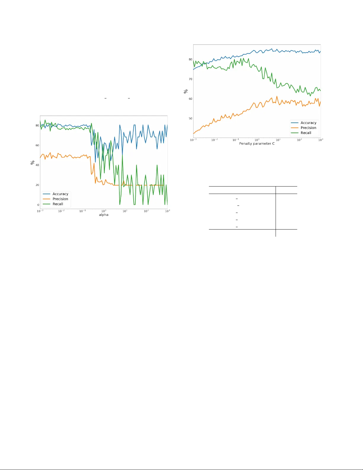
A udio Spectr ogram F actorization f or Classification of T elephony Signals below the A uditory Thr eshold Iroro Orife, Shane W alk er and Jason Flaks Marchex Inc., 520 Pik e, Seattle, W A, 98101 Abstract T raf fic Pumping attacks are a form of high-volume SP AM that target telephone networks, defraud customers and squander telephony resources. One type of call in these attacks is characterized by v ery low-amplitude signal lev els, notably belo w the auditory threshold. W e propose a technique to classify so-called “dead air” or “silent” SP AM calls based on features deriv ed from factorizing the caller audio spectrogram. W e describe the algorithms for feature extraction and classification as well as our data collection methods and production performance on millions of calls per week. Index T erms : audio spectrogram, matrix factorization, random forests, spam ov er ip telephony 1 Introduction The Public Switched T elephone Network (PSTN) is a collection of interconnected telephone netw orks that abide by the International T elecommunication Union (ITU) stan- dards allo wing telephones to intercommunicate. In re- cent decades, telephone service providers hav e modernized their network infrastructure to V oice ov er Internet Proto- col (V oIP) to take advantage of the a v ailability of equip- ment, lower operating costs and increased capacity to pro- vide voice communication and multimedia sessions. These advances also make it easy to automate the distribution of unsolicited and infelicitous call traffic colorfully known as robocalling or SP am over I nternet T elephony (SPIT) [28, 15]. For a comprehensive background on the ecosys- tem, pervasi v eness of telephone SP AM, the v arious actors and the impact to consumers, refer to [20, 26]. T raf fic Pumping (TP) is one class of robocall that starts when small, usually rural, Local Exchange Carriers (LXC) partner with telephone service providers (typically with toll- free numbers) to route the latter’ s calls. The LXC flood their own telephone netw orks with call traffic to boost their call volume and the inter-carrier re venue-sharing fees they are owed by long-distance, cross-regional Intere xchange Carriers (IXC), per the T elecommunications Act of 1996 [29, 5]. Confusing matters further , in the call-routing chain each carrier only sees the preceding and follo wing carrier . Therefore, no single player has the full route back to the spammer , which complicates provenance tracking and com- pletely stopping TP [4]. The telephon y stack behind the Marchex call and speech analytics business handles ov er one million calls per busi- ness day , or decades of encrypted audio recordings per week [23]. This volume makes our telephony stack particularly susceptible to attempts to anonymously establish automated voice sessions. TP caller audio has a number of dif ferent qualitativ e characteristics, it may be recordings (e.g. a sec- tion of an audio-book or music), broadband noise or signal- ing tones (e.g. busy , ring, fax, modem). The caller audio may also simply be “dead air”, where no one answers and there is no audible sound. By this, we do not suggest digital silence , but v ery low le v el signal lev els belo w the thresh- old of audibility . De v eloping countermeasures for this latter category of “silent” signal is focus of this report. Effecti vely mitigating TP is an adversarial match with the spammer . As countermeasures are deplo yed, spammers are motiv ated to find new means to dynamically e v ade. Inbound calls also require immediate attention, which at scale introduces real-time constraints on SP AM classifiers. W e contrast this with email SP AM mitigation which can often be deferred for future analysis offline. Finally , our call based business requires very high accurac y , as false positiv es, i.e. mistakenly blocked calls, are detrimental to our customers [20]. The main contributions of this paper are as follo ws: • W e propose a novel countermeasure for “dead air” V oIP SP AM using features deri ved from the Singular V alue Decomposition (SVD) of the audio spectrogram. • Gi v en the first tw o seconds of a call, we demonstrate the efficac y of a Random Forest classifier trained on these features to classify SP AM at production scale. This paper is organized as follo ws, Section 2 briefly summa- rizes related work mitigating SP AM. Section 3 details the algorithms for audio feature extraction. Section 4 describes our use of Random Forests for classification. Section 5 and 6 detail our experiments and results, while Section 7 discuss our post-attack experiments. Section 8 concludes with ideas for future work. 2 Related W ork V oIP SP AM countermeasures broadly fall into two cat- egories. The first in volves the use of Call Request Header (CRH) metadata e.g. Caller ID or caller’ s terminal device, in concert with white and black lists. Previous behavior and reputation systems also use Caller ID to track behavior and reputation scores. Howe ver CRH metadata is not al- ways present nor reliably propagated while Caller ID num- bers can be easily and cheaply falsified with open-source V oIP PBX systems such as Asterix PBX or FreeSWITCH [27, 21]. The second approach in v olves training machine-learned models to classify calls based on telephony control signal features or the call audio itself. When the call audio is based on a recording, landmark-based audio fingerprinting (e.g. music-id app Shazam) is commonly used for identification [6, 24]. Acoustic pattern analysis features include voice- codec signatures, { V oIP vs. PSTN } pack et loss patterns or channel noise-profiles [1, 20]. These systems are often cou- pled with interactiv e challenge-response tests (e.g. Audio- CAPTCHAs or Interactive voice response (IVR) “T uring tests”) to further verify the identity of suspicious callers and minimize false positi ves. For our specific task with “dead air” audio, we know of only one related ef fort, which focused on mobile de- vice identification using Mel-frequency cepstral coefficients (MFCC) features. T o account for the absence of an audible speech signal, Jahanirad et al. computed the entropy of the Mel-cepstrum, discovering that sections of “silent” signal resulted in high-valued entropy-MFCC features which were effecti ve in discriminating between dif ferent mobile device models [8]. This w ork suggests there are characteristic fea- tures of a source de vice or the transmission channel e v en in the absence of a speech signal. 3 F eatur e Extraction In telephony audio, background noise le v els can have a fair amount of energy , so simple energy heuristics do not ef- fectiv ely identify “silence”. This observ ation informed in- vestigations be yond simple activity detection models. The mission was now to find discriminable features given the first two seconds of a “silent” call. This short duration w as chosen because it can fit within the cadence of an extra ring- ing tone. Analyses of the audio rev ealed no dominant har- monicity , fundamental frequencies nor reliable temporal en- velope descriptions. Zero crossing and spectral shape statis- tics required a minimum signal le v el above the noise-floor to be of an y use as an input to a machine learning classifier [8]. In other words, peak lev els at -50 dBFS and average lev els around -72 dbFS in our 16-bit system corresponded to a very low dynamic range and a minimum signal-to-noise ratio, which limited the signal analysis options. 3.1 Spectrogram Representation Spectrograms are two dimensional representations of se- quences of frequency spectra with time along the horizon- tal axis and frequency along the vertical. The color and/or brightness illustrates the magnitude of the frequency k at time-frame n . A spectrogram compactly addresses the need to represent a sequence of audio features over the two sec- ond duration required for the task. Empirically , they are a practical choice, possessing more information that any sin- gle audio feature in v estigated abo ve, b ut with lo wer dimen- sionality than the time domain wa veform [30]. T o compute the spectrogram, we decode the first two seconds of mono 8kHz µ -law audio from our V oIP PBX to 16-bit PCM and then use a Short Time Fourier Trans- form (STFT) to compute the complex-v alued spectrogram S c ( n, k ) with n and k as the time-frame and frequency bin indices respectiv ely: S c ( n, k ) = W 2 − 1 X l = − W 2 w ( l ) · x ( l + nh ) · e − 2 π ilk/W (1) T o compute the STFT , the audio signal x ( n ) is sliced into ov erlapping se gments of equal length, W samples wide. Each segment is offset in time by a hop size value h . A Hann or raised-cosine window w ( l ) is multiplied element- wise with each segment. This “windowing” acts a taper- ing function to reduce spectral leakage during Fast Fourier T ransforms (FFT) [11]. Finally , an FFT of size W is com- puted separately on each windowed waveform segment to generate a complex spectrogram [17]. The magnitude spec- trogram X ( n, k ) is the complex modulus of S c ( n, k ) . X ( n, k ) = | S c ( n, k ) | (2) For a complex number z , its comple x modulus is defined as | z | = p x 2 + y 2 , where x and y denote the real and imag- inary parts respecti vely . W e compute the magnitude spec- trogram rather than the power or mel-spectrogram, as we observed that the dynamic scale of the magnitude represen- tation better suited to low-intensity signals [22]. 2 3.2 Spectrogram Decomposition Spectrogram factorization has been widely used for its flexibility modeling compositional mixtures of sounds from disparate sources. Applications include source separa- tion [18], music information retrie v al, en vironmental sound classification [25], instrument timbre classification [10], drum transcription [13], de-re verberation [9] and noise- robust speak er recognition [7]. Because we are strictly looking to classify , not reco ver entire components, we conceptualize the “silent” audio magnitude spectrogram as an additiv e mixture of spectral basis vectors corresponding to various source and trans- mission channel factors. W e represent constituent elements thusly , in both frequenc y and time, assuming that only the scale of each spectral basis is time-variant [16]. There are different decompositions of a matrix based on its properties, e.g. square vs. rectangular , symmetric, non negati v e elements or positi v e eigen values. In applications where mixtures of sounds sources in multicomponent sig- nals are modeled by their distribution of time/frequency en- ergy , latent sources are recovered using Principal compo- nent analysis (PCA). This is accomplished by a singular value or eigen-decomposition of the autocorrelation matrix, X X T of the spectrogram X [13]. On the magnitude spectrogram, we use the Singular V alue Decomposition (SVD) because it yields a “deeper” factorization and produces unique factors. Additionally , singular v alues are useful in understanding the most impor - tant spectral bases [2]. The SVD of an n × m matrix X is the factorization of X into the product of three matrices: X = U D V T (3) frequency X Spectrogram time = frequency U basis spectra dimensions dimensions D weights dimensions dimensions V T time activations time where the columns of the n × d matrix U and the m × d ma- trix V consist of the left and right singular vectors, respec- tiv ely . D is a d × d diagonal matrix whose diagonal entries are the singular values of X , representing the “strength” of each spectral basis. 4 Classification T o classify spectral bases feature v ectors from U , we trained a Random F orest (RF) classifier . The latter is an en- semble learning method for supervised classification tasks. Ensembles are a divide-and-conquer approach where a group of “weak learners” band together to form a “stronger Figure 1. Log-frequency Power Spectrogram of first two seconds of a TP “silent” call. Po wer Spectrogram plotted for visualization learner”. RFs arise from a machine learning modeling tech- nique called a decision tree, i.e. our weak learner . For clas- sification, decision trees make predictions based on obser- vations about the feature data, represented by the branches, to judgements about the data’ s class, represented by the leav es. RFs work by constructing a multitude of random deci- sion trees during training, yielding the class that is the mode of all the classes. T o classify new objects from an input fea- ture vector , the latter is processed by each tree, which gi ves a classification or “v ote” for a particular class. The forest chooses the classification with the most v otes among all the trees in the forest. RFs are a good choice for our task because of superb ac- curacy on datasets of dif ferent sizes. They also less prone to balance error in the case that there are imbalances in the number of training examples for each class. In our case we hav e a lot more HAM 1 than SP AM. W e also considered how well they generalize (i.e. do not overfit) and their compu- tational performance during prediction [3]. In contrast to linear support vector machine classifiers, see Figures 2-4, with RFs we were able to obtain good precision and busi- ness acceptable recall. 5 Experiments During a TP attack, an extra 10,000 to 33,000 “silent” calls per day may be handled by the telephony stack. Busi- ness requirements specified that tw o seconds was the maxi- mum permissible latency for this category of SP AM analy- sis before bridging calls. T o label calls: • W e enabled the call processors to write the first two sec- onds of audio data to disk during the collection period. 1 HAM are desirable calls, in contrast to SP AM 3 Each audio file was named with a unique call-id. • W e used a metric called Caller Speech (CS) emitted by the V oice Activity Detector (V AD) in our downstream ASR system [23] to find call-ids with zero Caller Speech. This latter metric tracks the number of times the V AD activ ates to capture caller utterances. For “dead air” calls, this v alue was always zero. Because we compute CS after the call has ended, this technique was only useful to select calls for labeling training data. W e collected 8,000 calls during one day during the at- tack, filtering calls that f ailed the IVR T uring test in concert with zero CS fields, we were able to quickly and definitiv ely label 256 “silent” SP AM calls. Another 692 failed the IVR test and had null CS v alues, but exhibited the same “dead” air features upon manual inspection. W e also labeled 1,500 calls with positiv e CS values that successfully passed the IVR test. For feature extraction, we used the Python frameworks, numpy and libr osa [12]. For classification, we used the scikit-learn RandomForestClassifier [14], trained for 100 iterations on the top 3 bases of U (Section 3.2). For cross v alidation, we used a stratified shuffle split cross- validator over the total number of trees, i.e. the data is shuf- fled each time, before a new train/test split is generated. Re- fer to Figure 2. T o establish a baseline performance with other classi- fiers, we experimented with tw o other linear models in scikit-learn , see T able 1. The first is the Linear Support V ec- tor Classification, LinearSVC , which uses a liblinear implementation that penalizes the intercept and minimizes the squared hinge loss. The second is SGDClassifier which optimizes the same cost function as LinearSVC but with the hinge loss and stochastic gradient descent in lieu of exact gradient descent. While both are linear kernel methods, the first is optimized to scale to a large number of samples, while the second supports minibatch training and may generalize better [14]. 6 Initial Results Evaluating the system performance entails comparing the model’ s predicted value to ground truth. There are four possible outcomes of the system’ s performance: A T rue Positiv e (TP) is a correct SP AM prediction, a T rue Ne gati ve (TN) is a correct HAM prediction. A False Positive (FP) is an incorrect SP AM prediction, a False Ne gati v e (FN) is a incorrect HAM classification, i.e. an actual SP AM call was able to get through. Precision, also known as positi ve predicti v e v alue, is the percentage of positi ve SP AM classifications that were ac- tually SP AM. Intuiti vely , precision tells us how correct the Figure 2. Stratified shuffle split cross-validation re- sults over the number of trees in the forest for RandomForestClassifier classifier is when it predicts that a call is SP AM. Precision suffers as the number of FPs gro w . Similarly , recall, also called sensitivity , tells us how many of the positive cases did the classifier get from the total number of positiv e cases. Recall suffers as the number of FNs gro w . Accurac y is the proportion of correctly identified calls (TP + TN) to all calls. P r ecision = T P T P + F P (4) Recal l = T P T P + F N (5) From a high-volume business perspecti ve, it is much less egre gious to let in the occasional SP AM call (FN), than it is to label and reject legitimate calls as SP AM (FP). In other words, high precision (low FPs) is more important than high recall (low FNs). Model Precision Recall Accuracy Linear SVC 58.57 63.60 84.04 Linear SVC with SGD 81.85 52.56 76.31 Random For est 83.82 63.27 90.40 T able 1. Classifier performance In e xamining the precision and recall figures from cross- validation, a model of 100 trees was chosen for production to foremost optimize precision (84%) and ov erall accuracy (90%). This practical choice was also influenced by our recognition of the limits and biases of our small and class imbalanced dataset. 4 As the realtime and low-latency requirements for classi- fication across thousands of concurrent calls made any kind of manual verification v ery impractical, to further minimize hanging up on real customers (FPs), we introduce the minor incon v enience of an IVR T uring test for all positiv e SP AM predictions, requiring callers to press a randomly chosen numeric ke y to proceed. Calls that do not make it past the IVR are labeled as REJECTED CALLER SILENCE in the production call-log. Figure 3. Stratified shuffle split cross-validation results ov er the re gularization term alpha , for SGDClassifier , an SVM classifier with SGD training 7 Post-Attack Experiments The nature of TP attacks is such that the y are high inten- sity over a short period of time, from days to weeks, after which SP AM levels subside, returning to a “steady-state” or low-grade level. This reduction could be externally mo- tiv ated or in response to our blocking ef forts. After this “dead air” attack abated, to re-ev aluate the performance of the classifier and understand any new characteristics of the low-pre valence SP AM, we captured a full day of audio from calls on a single production host, some 69,900 calls. Of these, 3,096 were marked as a kind of SP AM (not just “silent”) by the classifiers on that host. Cross-referencing these calls with call-stack metadata gav e us 968 confirmed calls for which we had both audio and a metadata tag of SP AM that had been rejected (i.e. the call-stack hung up or the call failed IVR Turing test). T able 2 lists the prev a- lence of dif ferent kinds of SP AM, with “silent” SP AM in boldface. After matching 968 rejected calls, we were left with 2,128 calls which were not rejected by the call-stack, all Figure 4. Stratified shuffle split cross-validation results ov er the penalty parameter C , for a LinearSVC Spam T ype Count CALLER F AX 611 CALLER SILENCE 233 CALLER RECORDING 87 CALLER NOISE 32 CALLER BUSY 5 T otal 968 T able 2. Pre v alence of SP AM types in 968 post-attack calls captured on one host of which were classified by our model as “silent” SP AM. This e xtremely high count of predicted “silent” SP AM calls suggested a very high FP rate and that our error analysis was far from complete. T abulating the call result metadata for each of the 2,128 predicted “silent” calls revealed a v ariety of outcomes, other than failing to pass the IVR T uring test. Most notable were calls which ended during the IVR T uring test or were bridged only to be ended by the caller an yway . Only 363 were ended by the agent. In T able 3 we enumerate all other ways a predicted “silent” call was ended. This error anal- ysis elucidates the distribution of errors and notably what kinds of audio calls were FP . Most surprisingly , once we started programmatically an- alyzing audio predicted as “silent” SP AM, regardless of whether it was rejected or abandoned by the agent/caller , 98.6% { 2100/2128, 229/233 } of all predicted “silent” calls were, in this post-attack test, pure digital silence! There are many conditions under which digital silence is correctly produced by the call-stack, for example at the be- 5 Call Result Ended By Count BRIDGED CALLER 1159 IVR ABANDON CALLER 547 BRIDGED A GENT 363 BRIDGE ABANDON CALLER 37 BRIDGE TIMEOUT APP 13 NO ELIGIBLE A GENTS APP 4 BRIDGE TIMEOUT CALLER 2 BRIDGE ABANDON A GENT 1 NO ELIGIBLE A GENTS CALLER 1 BRIDGE OUT OF SER VICE APP 1 T able 3. Reasons 2,128 “silent” calls were ended ginning of HAM and some SP AM calls, during transfers or right before a ring tone. Our error analysis illuminated the fact that digital silence needed to have been better consid- ered when labeling call se gments. Had we recognized the prev alence and interplay with “dead air” silence, we would hav e labeled calls with mixtures differently , at a finer reso- lution or factored out any digital silence from positive “dead air” training segments. This shift in the distribution of audio features between the training and test phases versus running “in the wild”, ov er time, raises questions about the steady-state efficac y of the classifier and the need to k eep the model up to date in this adversarial match. These questions are common in machine learning practice, i.e. when an algorithm is trained in a lab setting without seeing the full breadth of data from the production system, carefully formulated questions must be asked and exhausted to ensure that models continue to perform satisfactorily . 8 Future W ork In addition to the practical machine learning matters and keeping the SP AM classifiers regularly updated, there are a number of interesting algorithmic av enues for future work. These include v arious neural network alternati ves to non- negati v e matrix factorization (NMF) [19] as well as fine- tuned, state of art image classification models [31]. Fine- tuning is the process of a trained model’ s architecture and weights as a starting point, freezing lower layers and train- ing on our smaller “silent” spectrograms dataset. Adv er - sarial issues aside, these techniques have the potential to alleviate the need for an interactive IVR Turing test in pro- duction. 9 Acknowledgement The authors thank the follo wing Marchex colleagues for their efforts on data collection and system deployment: Dav e Olsze wski, Ryan O’Rourke and Sha wn W ade. References [1] V . A. Balasubramaniyan, A. Poonawalla, M. Ahamad, M. T . Hunter , and P . T raynor . Pindr0p: using single- ended audio features to determine call provenance. In A CM Conference on Computer and Communications Security , 2010. [2] C. Boling and K. Das. A comparison of svd and nmf for unsupervised dimensionality reduction, 2015. [3] L. Breiman and A. Culter . Random forests. https: //www.stat.berkeley.edu/ ˜ breiman/ RandomForests/cc_home.htm#intro , 2004. [4] Dialogtech. Industry Problem: Putting a Stop to T raf fic Pumping Spam Calls. https://tinyurl. com/ybkfgbuw , 2015. [5] FCC. T raffic pumping. https://www.fcc.gov/ general/traffic- pumping , 2015. [6] G. Grutzek, J. Strobl, B. Mainka, F . Kurth, C. P ¨ orschmann, and H. Knospe. A perceptual hash for the identification of telephone speech. In ITG F achbericht 236: Sprac hkommunikation, VDE V er- lag , volume 10, Braunschweig, 2012. ITG Sympo- sium Speech Communication. [7] A. Hurmalainen, R. Saeidi, and T . V irtanen. Noise ro- bust speaker recognition with conv oluti v e sparse cod- ing. In Sixteenth Annual Confer ence of the Interna- tional Speech Communication Association , 2015. [8] M. Jahanirad, A. W . A. W ahab, N. B. Anuar , M. Y . I. Idris, and M. N. A yub . Blind source mobile device identification based on recorded call. Engineering Ap- plications of Artificial Intelligence , 36:320–331, 2014. [9] A. Juki ´ c, N. Mohammadiha, T . van W aterschoot, T . Gerkmann, and S. Doclo. Multi-channel lin- ear prediction-based speech derev erberation with low- rank po wer spectrogram approximation. In Acoustics, Speech and Signal Processing (ICASSP), 2015 IEEE International Conference on , pages 96–100. IEEE, 2015. [10] A. Kaminiarz and E. Łukasik. Mpeg-7 audio spec- trum basis as a signature of violin sound. In Signal Pr ocessing Conference , 2007 15th Eur opean , pages 1541–1545. IEEE, 2007. [11] D. A. L yon. The discrete fourier transform, part 4: spectral leakage. Journal of object technolo gy , 8(7), 2009. 6 [12] B. McFee, C. Raffel, D. Liang, D. P . W . Ellis, M. McV icar, E. Battenberg, and O. Nieto. librosa: Au- dio and music signal analysis in python. 2015. [13] I. Orife. Riddim: A rhythm analysis and decompo- sition tool based on independent subspace analysis. arXiv pr eprint arXiv:1705.04792 , 2001. [14] F . Pedregosa, G. V aroquaux, A. Gramfort, V . Michel, B. Thirion, O. Grisel, M. Blondel, P . Prettenhofer , R. W eiss, V . Dubourg, J. V anderplas, A. Passos, D. Cournapeau, M. Brucher, M. Perrot, and E. Duch- esnay . Scikit-learn: Machine Learning in Python . Journal of Machine Learning Resear c h , 12:2825– 2830, 2011. [15] J. Rosenberg and C. Jennings. The session initiation protocol (sip) and spam. T echnical report, 2008. [16] T . Sakata. Applied Matrix and T ensor V ariate Data Analysis . Springer , 2016. [17] scip y .signal. SciPy v1.0.0 Reference Guide Signal processing (scipy .signal. https://docs.scipy. org/doc/scipy/reference/generated/ scipy.signal.hanning.html#scipy. signal.hanning , 2008. [18] P . Smaragdis, B. Raj, and M. Shashanka. Supervised and semi-supervised separation of sounds from single- channel mixtures. Independent Component Analysis and Signal Separation , pages 414–421, 2007. [19] P . Smaragdis and S. V enkataramani. A neural net- work alternative to non-negati v e audio models. CoRR , abs/1609.03296, 2016. [20] H. T u, A. Doup ´ e, Z. Zhao, and G.-J. Ahn. Sok: Ev- eryone hates robocalls: A surv ey of techniques against telephone spam. In Security and Privacy (SP), 2016 IEEE Symposium on , pages 320–338. IEEE, 2016. [21] A. K. V enkatasubbareddy , K. K. Sadasiv am, and P . Kannappan. Implementation of progressiv e multi gray-lev eling. [22] T . V irtanen. Spectrogram f actorization methods for audio processing. Univ ersity Lecture, 2017. [23] S. W alker , M. Pedersen, I. Orife, and J. Flaks. Semi-supervised model training for unbounded con- versational speech recognition. arXiv pr eprint arXiv:1705.09724 , 2017. [24] A. W ang et al. An industrial strength audio search algorithm. In Ismir , volume 2003, pages 7–13. W ash- ington, DC, 2003. [25] B. W ang and M. D. Plumbley . Musical audio stream separation by non-ne gati ve matrix factorization. In Pr oc. DMRN summer conf , pages 23–24, 2005. [26] W ikipedia. Phone fraud. https://en. wikipedia.org/wiki/Phone_fraud ,, 2004. [27] W ikipedia. Caller ID spoofing. https: //en.wikipedia.org/wiki/Caller_ID_ spoofing , 2006. [28] W ikipedia. V oIP spam. https://en. wikipedia.org/wiki/VoIP_spam , 2007. [29] W ikipedia. T raf fic pumping. https://en. wikipedia.org/wiki/Traffic_pumping , 2011. [30] L. W yse. Audio spectrogram representations for pro- cessing with con v olutional neural networks. arXiv pr eprint arXiv:1706.09559 , 2017. [31] F . Y u. A comprehensi ve guide to fine-tuning deep learning models in keras. https: //flyyufelix.github.io/2016/10/03/ fine- tuning- in- keras- part1.html , 2016. 7