Comparison of VCA and GAEE algorithms for Endmember Extraction

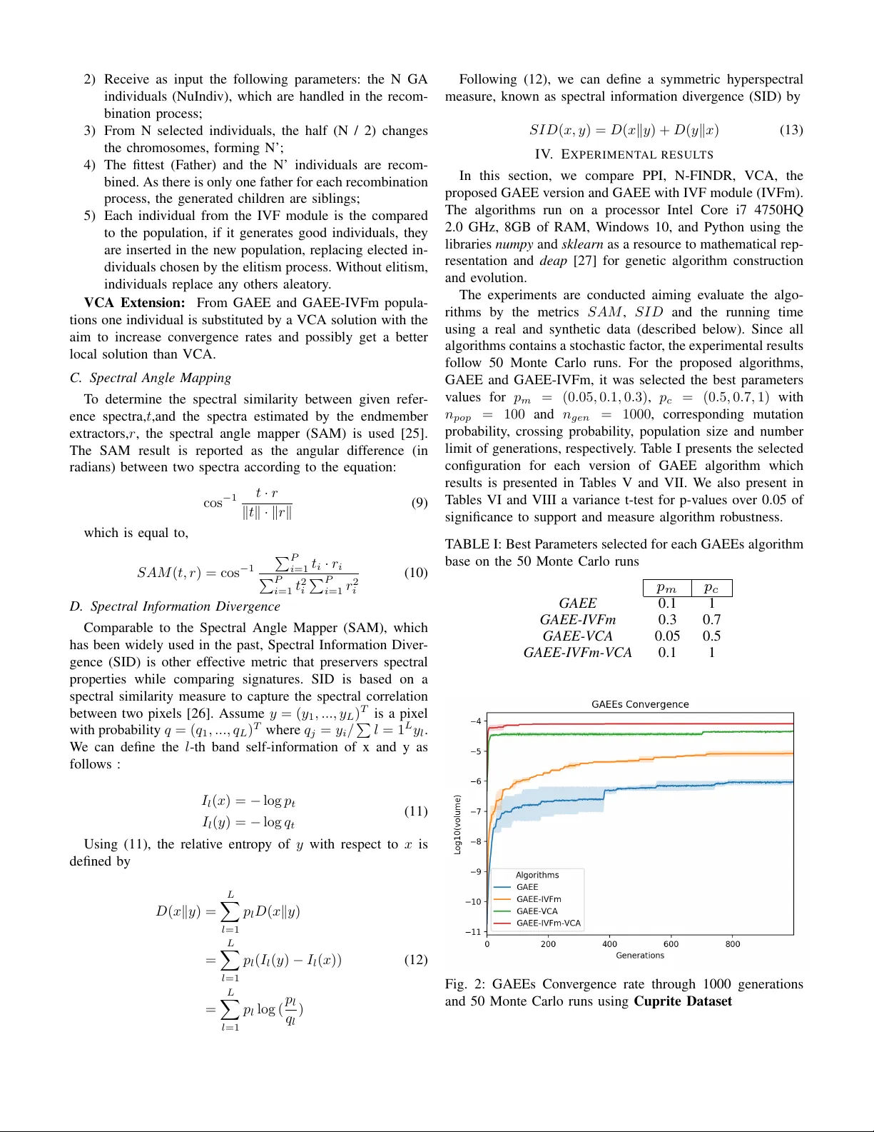
Comparison of VCA and GAEE algorithms for Endmember Extraction Douglas W inston. R. S. Informatics Institute (INF) Federal Univ ersity of Goi ´ as (UFG) Goi ˆ ania, Brazil douglas.winston@acm.org Gustav o T . Laureano Informatics Institute (INF) Federal Univ ersity of Goi ´ as (UFG) Goi ˆ ania, Brazil gustav o@inf.ufg.br Celso G. Camilo Jr . Informatics Institute (INF) Federal Univ ersity of Goi ´ as (UFG) Goi ˆ ania, Brazil celso@inf.ufg.br Abstract —Endmember Extraction is a critical step in hyper - spectral image analysis and classification. It is an useful method to decompose a mixed spectrum into a collection of spectra and their corresponding proportions. In this paper , we solve a linear endmember extraction problem as an evolutionary optimization task, maximizing the Simplex V olume in the endmember space. W e propose a standard genetic algorithm and a variation with In V itro F ertilization module (IVFm) to find the best solutions and compare the results with the state-of-art V ertex Component Analysis (VCA) method and the traditional algorithms Pixel Purity Index (PPI) and N-FINDR. The experimental results on real and synthetic hyperspectral data confirms the over come in performance and accuracy of the proposed approaches over the mentioned algorithms. Index T erms —hyperspectral, linear mixing model, endmember extraction, genetic algorithm, remote sensing I . I N T R O D U C T I O N T H E prior few years hav e observed considerable advances in hyperspectral imaging where statistical signal processing has performed a central role in pushing algorithm design and de velopment for hyperspectral data exploitation [1]. It has brought the attention of those who come from various disciplinary areas by searching new applications and making associations between remote sensing and other engineering disciplines [2]. The hyperspectral image has matured to a rapidly growing technique in remote sensing image processing due to recent advances in hyperspectral imaging technology . It makes use of hundreds of contiguous spectral bands expanding the capacity of multispectral sensors using dozens of discrete spectral bands [3]. Ne vertheless, in real applications, pixels may contain a mixture of spectra resulting from the combination of multiple substances, named endmembers, in v aried ab undance fractions. In this situation, the diffused energy is a mixing of the endmember spectra [4]. A challenging assignment underlying hyperspectral applications is the spectral unmixing which describes the decomposition of a mixed pixel into a collection of reflectance spectra called endmember signatures, and the corresponding abundance fractions. Depending on the type of mixing at each pixel, the pixel- mixed model can be separated into two classes, linear mixed model, and nonlinear mixed model [5]. The linear model considers that a mixed pixel is a linear combination of end- member signatures weighted by their correspondent ab undance fractions. The linear model is based on the assumption that the number of substances and their reflectance spectra are kno wn. Therefore, with those assumptions, hyperspectral unmixing is a linear problem for which many solutions have been proposed such as Con ve x Cone Analysis [6], Pixel Purity Index (PPI) [7], V erte x Component Analysis (VCA) [8], N-FINDER (N- FINDR) [9], Simplex Growing Algorithm (SGA) [10], and variations of those above [11][12][13][14]. Pixel purity index (PPI) is a traditional method for end- member extraction. The algorithm determines the endmembers and a pix el purity index by repeatedly projecting data into a set of random unit vectors [15]. Follo wed by , N-FINDR which finds a simplex of the maximum volume with a giv en number of vertices. The procedure begins with a random initial selection of pixels. If the v olume of the simplex increases with the new pixel, it is accepted as the new endmember [12]. Differently , the V ertex Component Analysis (VCA) is an unsupervised endmember extraction method that projects data onto a orthogonal direction to the subspace spanned by the endmembers already determined, which is based upon the notion that endmembers are simple x vertices and that the af fine transformation of a simplex is a simplex as well [8]. The Simplex Growing Algorithm (SGA) is an endmember finding algorithm which grows simplexes with maximal volume one verte x at a time to find new endmembers where Simplex V olumes (SV) are calculated by the determinants of respective endmember matrices [10]. Algorithms based on VCA hav e lo w computational com- plexity and accurate extraction results [16] but there are still sev eral weaknesses in these algorithms. One is the extraction accuracy will be reduced if the real data cannot meet the assumptions of the simplex structure or if there is an absence of pure pixels [17]. Furthermore, these algorithms generated the initial endmembers randomly , which is not an effecti ve way to the initialization and takes a long time to find a desired set of endmembers. In order to solve these problems, an integration of genetic algorithm (GA) and simplex volume maximization is proposed. In this paper , we formulate the endmember extraction 978-1-5386-5541-2/18/$31.00 c  2018 IEEE problem as a single objectiv e maximizing the volume of the simplex deri ved from the endmember matrix. It was believed that the ground-truth endmembers can be located by finding a collection of pixel vectors whose simplex volume is the largest [9]. The ev olutionary approach inserts greater flexibility in the con ver gence of the algorithm and is possible to reach a better set of pure pixels that best represents the data without relying only on the randomness of the selection phase imposed by interactiv e methods. Experiments on real hyperspectral images show the ef fectiveness of the proposed endmember extraction method with rather good computational complexity compared to other methods. The rest of this paper is or ganized as follo ws: Section II introduces some background knowledge of linear mixed model, endmember extraction, and e volutionary algorithms. Section III introduces the objectiv e function used, the proposed endmember extractor in details, and metrics used to compare the signatures results. Experimental study of real and synthetic is described in Section IV . Finally , concluding remarks are giv en in Section V . I I . B AC K G RO U N D W e will use the following notations throughtout the paper: • Y  R L represents the observed data matrix. L is the number of spectral bands, and N denotes the number of total pixels in the data matrix. • y  R L × 1 is the measured spectrum of a pixel. • M  R L is a endmember matrix containing p endmem- bers. • α  R P × 1 is a vector containing the fractional ab un- dances of the endmembers in the pixel. • n  R L × 1 is a vector collecting the errors af fecting the measuresments at each spectral band. A. Linear Mixing Model In the Linear mixing model (LMM), the spectral response of a pixel is a linear combination of all the pure spectral signature of endmembers present in the pix el [18]. When the endmembers are distributed as discrete paths, the LMM is certainly valid and different endmembers do not interfere with each other . Assuming the linear mixing scenario, each observed spectral vector is giv en by y i = p X j =1 m ij α j + n j (1) where y i denotes the measured reflectance of a pixel at spectral band i , m ij is the reflectance of the j th endmember at spectral band i , α j stands for the fractional abundance of the j th endmember , and n i represents noise and modeling errors for the spectral band i . If the data has L spectral bands, Eq. (1) can be rewritten as follows: y = M α + n (2) Owing to physical constraints, abundance fractions are non- negati ve ( α ≥ 0) and satisfy the positivity constraint 1 T α = 1 , Fig. 1: Illustration of the VCA algorithm [8]. where 1 is a P × 1 vector of ones. Each pixel can be vie wed as a vector in an L -dimensional Euclidean space, where each channel is assigned to one axis of space. Since α ∈ R P , 1 T α = 1 and ( α ≥ 0) construct a simplex, then Eq. (2) is also a simplex denotes by S x where x  R L and x = M α . B. V ertex Component Analysis The (VCA) algorithm unmix linear mixtures of endmember spectra by assuming n = 0 and construction a conv ex cone C p following: y = M γ α , 1 T α = 1 , ( α ≥ 0) and ( γ ≥ 0) where γ is a scale factor to model illumination variability . In Figure 1, the projecti ve projection of the con ve x cone C p onto a properly chosen hyperplane is a simplex with vertices corresponding to the vertices of the simplex S x . After identifying S p , the VCA algorithm iteratively projects data onto a direction orthogonal to the subspace spanned by the endmembers already determined. The ne w endmember signature corresponds to the extreme of the projection [8]. In the first iteration, data are projected onto the first direction f 1 . The extreme of the projection corresponds to endmember m a . In the next iteration, endmember m b is found by projecting data onto direction f 2 , which is orthogonal to m a . The algorithm iterates until the number of endmembers is exhausted. C. Genetic Algorithms Once the genetic representation and the fitness function are defined, a GA proceeds to initialize a population of solutions and then to improve it through repetiti ve application of the mutation, crossover , and selection operators. Section III-B will explain in details the choice of each operator mentioned and representation of chromosomes in respect to the linear mixing model and the hyperspectral data [19][20]. D. In V itr o F ertilization Module The Genetic Algorithm’ s e volutionary process is composed of a recurrent runs, each repetition produces a new generation. Concerning each fresh generation, indi viduals are created and injected into the population to succeed some of the current ones, which are dropped. Still, many of these eliminated individuals contain genes with information that is important for the search [21]. In V itro Fertilization Module (IVFm) recombines the chro- mosomes from the GA population with new individuals to bet- ter exploit information lost. The IVFm generates children from the recombination of chromosome parts of some individuals with the fittest one. If the process generates a better individual, this replaces the current best. Otherwise, if the operator does not produce a better individual, there is no interference in the population [22]. I I I . M E T H O D O L O G Y A. Simplex V olume Maximization In geometry , a simplex, also named a pentatope, is the generalization of a tetrahedral section of space to arbitrary n dimensions. A j -dimensional ( j + 1) -verte x simplex S j +1 is a con ve x polygon with j + 1 vertices. Therefore, a single point could be considered as a 1-vertex simplex and a 2-vertex simplex could be proclaimed as a line segment between two specified points. Moreov er , a 3-vertex simplex is a triangle, a 4-verte x simplex is a tetrahedron, etc [11] [23]. Suppose a ( j + 1) -v ertex simplex S j +1 where it can be expressed by the set of points as S j +1 = S ( m 1 , m 2 , ..., m j +1 ) (3) The content of volume of a simplex is denoted as V ( S j +1 ) . Let V ( S j ) denote the volume of a j -vertex simplex S j which is a base of a ( j + 1) -verte x simplex S j +1 and h j be the height of the apex from subspace containing the base S j . The volume V ( S j +1 ) can be simplified as V ( S n +1 ) = ( 1 n ! ) n Y j =1 h j = ( 1 n ! ) V ( P n ) (4) By the previous equation it can be seen that the volume of V ( S n ) of an n-simplex is ( 1 n ! ) of the volume of the corresponding ( n − 1) -vertices simplex. Now , consider an n -dimensional simplex S n with n + 1 vertices m 1 , m 2 , ...m n +1  R n (endmembers follo wing the hy- perspectral representation of a simplex). The volume of P n is determined by n edge vectors, M E = m 2 − m 1 , ...m n +1 − m 1 , corresponding to S n , it is the absolute value D et ( M E ) . V ( P n ) = | D et ( M E ) | = | D et [( m 2 − m 1 ) , ... ( m n +1 − m 1 )] | (5) Therefore, by (4) and (5), the volume V ( S n +1 ) of an ( n + 1) -simplex S n +1 is expressed as V ( S n +1 ) = ( 1 n ! ) V ( P n ) = ( 1 n ! ) | D et ( M E ) | (6) Using elementary column operation of matrix and properties of the determinant for a block matrix, D et [ M E ] is obtained by D et  1 1 ... 1 m 1 m 2 ... m n +1  D et [ m ∗ 2 , m ∗ 3 , ..., m ∗ n +1 ] (7) Then, V ( S n +1 ) = ( 1 n ! ) D et [ m ∗ 2 , m ∗ 3 , ..., m ∗ n +1 ] (8) It is deserving noting that the volume deriv ed by (8) is only possible while M E is square matrix. Consequently a dimensionality reduction is necessary , in this paper , it was adoted the Principal Component Analysis (PCA) [24]. B. Genetic Algorithm Endmember Extractor Coding Scheme: In this paper , a chromosome is designed by having m genes where m represents the number of end- members defined previously by the user or a dimensionality estimation method. T o obtain a possible solution to the end- member extraction problem, each gene is considered to be an endmember (pure pixel) in the data, and each individual in the population is considered to be a combination of endmembers (pixels). T o generate a coding system, a vector of integer digits in the chromosome is designed where a gene equals to a pixel index in the hyperspectral data. Each endmember contributes to the calculation of a fitness function (Simplex V olume). Fitness function: Under the linear mixing model, the spectral data from a scene resides within a simplex in a mul- tidimensional space whose endmembers represent the vertices of the simplex, and the volume defined by the endmembers is maximal. Therefore, the objective is to find the maximum vol- ume among the set of all simplex es with the same dimension. The fitness function then is the calculation of the volume of a simplex expressed by the Eq. (8) Initialization: Population individuals are created by a ran- domly process where arbitrary pixels are chosen from the data matrix as individual’ s genes. Selection: T ournament selection is used to select three individuals at random from the population, each indi vidual selected goes through the mating process. [20]. Mating: A two-point crossov er is chosen for the mating process of indi viduals. The two indi viduals are modified in place and both keep their original length depending on a probability informed at the beginning of the ev olutionary process. Mutation: From a selected individual, randomly choose a new gene (Pixel) from the data matrix replacing the previous gene. The gene alteration depends on a probability defined at the inicialization of the GA paramenters. In V itro Fertilization Module: At the beginning of the GA execution the same population selected by the GA is then inject into the IVF module where each generation executes the following tasks [21]: 1) Find the fittest indi vidual and label it as Father; 2) Recei v e as input the follo wing parameters: the N GA indi viduals (NuIndi v), which are handled in the recom- bination process; 3) From N sel ected indi viduals, the half (N / 2) changes the chromosomes, forming N’; 4) The fittest (F ather) and the N’ indi viduals are recom- bined. As there is only one f ather for each recombination process, the generated children are siblings; 5) Each indi vidual from the IVF module is the compared to the population, if it generates good indi viduals, the y are inserted in the ne w population, replacing elected in- di viduals chosen by the elitism process. W ithout elitism, indi viduals replace an y others aleatory . VCA Extension: From GAEE and GAEE-IVFm popula- tions one indi vidual is substituted by a VCA solution with the aim to increase con v er gence rates and possibly get a better local solution than VCA. C. Spectr al Angle Mapping T o determine the spectral similarity between gi v en refer - ence spectra, t ,and the spectra estimated by the endmember e xtractors, r , the spectral angle mapper (SAM) is used [25]. The SAM result is reported as the angular dif ference (in radians) between tw o spectra according to the equation: cos − 1 t · r k t k · k r k (9) which is equal to, S AM ( t, r ) = cos − 1 P P i =1 t i · r i P P i =1 t 2 i P P i =1 r 2 i (10) D. Spectr al Information Diver g ence Comparable to the Spectral Angle Mapper (SAM), which has been widely used in the past, Spectral Information Di v er - gence (SID) is other ef fecti v e metric that preserv ers spectral properties while comparing signatures. SID is based on a spectral similarity measure to capture the spectral correlation between tw o pix els [26]. Assume y = ( y 1 , ..., y L ) T is a pix el with probability q = ( q 1 , ..., q L ) T where q j = y i / P l = 1 L y l . W e can define the l -th band self-information of x and y as follo ws : I l ( x ) = − log p t I l ( y ) = − log q t (11) Using (11), the relati v e entrop y of y with respect to x is defined by D ( x k y ) = L X l =1 p l D ( x k y ) = L X l =1 p l ( I l ( y ) − I l ( x )) = L X l =1 p l log ( p l q l ) (12) F ollo wing (12), we can define a symmetric h yperspectral measure, kno wn as spectral information di v er gence (SID) by S I D ( x, y ) = D ( x k y ) + D ( y k x ) (13) I V . E X P E R I M E N T A L R E S U L T S In this section, we compare PPI, N-FINDR, VCA, the proposed GAEE v ersion and GAEE with IVF module (IVFm). The algorithms run on a processor Intel Core i7 4750HQ 2.0 GHz, 8GB of RAM, W i ndo ws 10, and Python using the libraries numpy and sklearn as a resource to mathematical rep- resentation and deap [27] for genetic algorithm construction and e v olution. The e xperiments are conducted aiming e v aluate the algo- rithms by the metrics S AM , S I D and the running time using a real and synthetic data (described belo w). Since all algorithms contains a stochastic f actor , the e xperimental results follo w 50 Monte Carlo runs. F or the proposed algorithms, GAEE and GAEE-IVFm, it w as selected the best parameters v alues for p m = (0 . 05 , 0 . 1 , 0 . 3) , p c = (0 . 5 , 0 . 7 , 1) with n pop = 100 and n g en = 1000 , corresponding mutation probability , crossing probability , populati on size and number limit of genera tions, respecti v ely . T able I presents the selected configuration for each v ersion of GAEE algorithm which results is pres ented in T ables V and VII. W e also present in T ables VI and VIII a v ariance t-test for p-v alues o v er 0.05 of significance to support and measure algorithm rob ustness. T ABLE I: Best P arameters selected for each GAEEs algorithm base on the 50 Monte Carlo runs p m p c GAEE 0.1 1 GAEE-IVFm 0.3 0.7 GAEE-VCA 0.05 0.5 GAEE-IVFm-VCA 0.1 1 Fig. 2: GAEEs Con v er gence rate through 1000 generations and 50 Monte Carlo runs using Cuprite Dataset A. Cuprite Dataset Cuprite is the most benchmark dataset for the hyperspectral unmixing research that covers the Cuprite in Las V eg as, NV , U.S. There are 224 channels, ranging from 370 nm to 2480 nm . After removing the noisy channels (1–2 and 221–224) and water absorption channels (104–113 and 148–167), we remain 188 channels. A region of 250 × 190 pixels is considered, where there are 14 types of minerals. Since there are minor differences between v ariants of similar minerals, the number of endmembers is reduce to 12, which are summarized as follows ”#1 Alunite”, ”#2 Andradite”, ”#3 Buddingtonite”, ”#4 Du- mortierite”, ”#5 Kaolinite1”, ”#6 Kaolinite2”, ”#7 Muscovite”, ”#8 Montmorillonite”, ”#9 Nontronite”, ”#10 Pyrope”, ”#11 Sphene”, ”#12 Chalcedony”. The T ables V and VII sho w the mean of SAM and SID distances for the Cuprite Dataset after 50 runs. From these results, we can observe that GA based algorithms overcame VCA, PPI and N-FINDR results in most of the extracted endmembers, with advantage for the GAEE algorithm. The GAEE-IVFm tends to approximate to GAEE achieving best results in some endmembers. The addition of endmember hint in GAEE-VCA and GAEE-IVFm-VCA does not contribute significantly to achiev e best results compared with GAEE algorithm but approximate the metrics with a considerable reduction in population size and number of generations, such as the GAEE-IVFm algorithm. Figure 2 shows GAEE high div ersity of individuals at early 200 generations while the extended VCA versions induce fast conv ergence but low div ersity . The last row of tables presents the Root Mean Squared (RMS) for both SAM and SID metrics. In T ables VI and VIII we noticed that GAEE had 7 . 92% gain ov er VCA with SAM metric and 24 . 37% gain with SID metric, but the VCA performs much faster than the ev olution- ary approaches. In Figure 3, the 12 extracted endmembers are shown for the interactive algorithms and the GAEE algorithm version with lowest RMS (GAEE-IVFm). B. Le gendr e Dataset Legendre Dataset is a set of hyperspectral synthetic images from the IC Synthetic Hyperspectral Collection. These images were constructed by the ”Synthesis tools” package [28]. All these synthetic images hav e been generated using fiv e selected endmembers from the USGS spectral library included in the ”Synthesis tools” package. Each image’ s spatial dimensions are of 128 pixels and they hav e 431 spectral bands. In this paper three additive noise versions of the legendre dataset has been used, with Signal to Noise Ratios (SNR) of 20, 40 and 80 dB, respectiv ely . T ables II and III show both SAM and SID distances for the three synthetic images generated by the endmember extractors. It can be noticed that GAEE-IVF had the best results among all algorithms except in the image with low SNR (20db) due to option of not using a dimentionality reduction or noise filter on the ev olutionary process. Other evolutionary versions performed similar to GAEE-IVF and better than VCA in high SNR. T able IV presents the SAM gain over the methods used in the comparison. In the case where the SNR is 40 dB, the GAEE-IVF has 84% of gain and 114% over images with SNR of 80 dB. In Figure 4a and 4b is possible to notice that the GAEE-IVF extracted the right pure pixel as endmember , but the additiv e noise contributed to the low SAM distance. Howe ver , the SID distances were best for the e volutionary algorithm GAEE-IVF with a VCA initial individual’ s solution is added to the GAEEs population. T ABLE II: Root Mean Squares SAM Distance Between Ex- tracted Endmembers and Laboratory Reflectances for Legen- dre Dataset with Signal Noise Ratio of 20, 40 and 80 dB 20 dB 40 dB 80 dB PPI 0.3348 0.2474 0.1281 N-FINDR 0.1312 0.0685 0.0691 VCA 0.0851 0.0660 0.0691 GAEE 0.0924 0.0424 0.0412 GAEE-IVFm 0.0939 0.0375 0.0354 GAEE-VCA 0.1212 0.0559 0.0691 GAEE-IVFm-VCA 0.0971 0.0544 0.0496 T ABLE III: Root Mean Squares SID Distance Between Ex- tracted Endmembers and Laboratory Reflectances for Legen- dre Dataset with Signal Noise Ratio of 20, 40 and 80 dB 20 dB 40 dB 80 dB PPI 34.9975 19.8908 6.3210 N-FINDR 3.3918 7.7910 8.2932 VCA 2.8671 7.5158 8.2847 GAEE 2.4536 3.7487 4.0112 GAEE-IVFm 2.5987 1.4021 1.4814 GAEE-VCA 2.5749 6.7584 8.2933 GAEE-IVFm-VCA 1.6756 2.6890 3.6275 T ABLE IV: GAEE-IVFm SAM Gain Comparison for Legen- dre Dataset with Signal Noise Ratio of 20, 40 and 80 dBs 20 dB 40 dB 80 dB PPI 298.45% 988.78% 454.87% N-FINDR 26.11% 96.26% 114.40% VCA -42.25% 84.86% 114.39% GAEE -0.43% 17.18% 22.16% GAEE-IVFm - - - GAEE-VCA 16.81% 78.16% 114.40% GAEE-IVFm-VCA 3.22% 33.26% 19.50% V . C O N C L U S I O N This paper discussed the possible application of an e volu- tionary algorithm (GAEE) 1 and its variation (GAEE-IVFm) to the problem of finding a set of endmembers with maximal volume in a hyperspectral image. First, from the concepts detailed by the V ertex Component Analysis and the Linear Mixing Model it was possible to construct a genetic model of the hyperspectral data, setting a simplex representation for the datasets and performing a selection of pure pixels in each generation until a limit is reached. The results of GAEE were 1 The proprosed methods are av ailable at https://github.com/haruto- boshi/GAEE superior to the state-of-art method VCA with 7.92% gain for the Cuprite dataset with SAM metric and ov er 84% gain for the synthetic data with SNR of 40 dB and 114% of gain for 80 dB. GAEE-IVFm was considered a superior method while w orking with synthetic images, since the presence of pure pixels (endmembers) and the linear mixing model are guaranteed by its construction. The methods dev eloped in this paper obtained inferior results in the synthetic dataset with SNR of 20 db. The inferior results are due to the fact that the e volutionary approaches do not make use of projections or dimentionality reduction, differently from VCA, which reduces the noise factor . An immediate next step for this research is to dev elop a noise filter as post processing of the results for images with low Signal Noise Ration. In Addition, the linear mixing model could be replaced by a non- linear kernel, then eliminating the necessity of pure pixels on the image. Consequently , the choice of a new ev olutionary fitness function w ould reduce the computational comple xity improving GAEEs performance. R E F E R E N C E S [1] L. W ang and C. Zhao, Hyperspectral Image Pr ocessing . Springer . [2] C.-I. Chang, Hyperspectral data exploitation: theory and applications . John Wiley & Sons, 2007. [3] D. Manolakis and G. Shaw , “Detection algorithms for hyperspectral imaging applications, ” IEEE signal pr ocessing magazine , vol. 19, no. 1, pp. 29–43, 2002. [4] M. Fauv el, Y . T arabalka, J. A. Benediktsson, J. Chanussot, and J. C. T ilton, “ Advances in spectral-spatial classification of hyperspectral im- ages, ” Pr oceedings of the IEEE , vol. 101, no. 3, pp. 652–675, 2013. [5] L. Zhao, M. Fan, X. Li, and L. W ang, “Fast implementation of linear and nonlinear simplex growing algorithm for hyperspectral endmember extraction, ” Optik-International Journal for Light and Electr on Optics , vol. 126, no. 23, pp. 4072–4077, 2015. [6] A. Ifarraguerri and C.-I. Chang, “Multispectral and hyperspectral image analysis with conve x cones, ” IEEE transactions on g eoscience and r emote sensing , vol. 37, no. 2, pp. 756–770, 1999. [7] C.-I. Chang and A. Plaza, “ A fast iterative algorithm for implementation of pixel purity index, ” IEEE Geoscience and Remote Sensing Letters , vol. 3, no. 1, pp. 63–67, 2006. [8] J. M. Nascimento and J. M. Dias, “V ertex component analysis: A fast algorithm to unmix hyperspectral data, ” IEEE transactions on Geoscience and Remote Sensing , vol. 43, no. 4, pp. 898–910, 2005. [9] M. E. Winter , “N-findr: An algorithm for fast autonomous spectral end- member determination in hyperspectral data, ” in Imaging Spectr ometry V , vol. 3753. International Society for Optics and Photonics, 1999, pp. 266–276. [10] C.-I. Chang, C.-C. W u, W . Liu, and Y .-C. Ouyang, “ A new grow- ing method for simplex-based endmember extraction algorithm, ” IEEE T ransactions on Geoscience and Remote Sensing , v ol. 44, no. 10, pp. 2804–2819, 2006. [11] L. Zhao, J. Zheng, X. Li, and L. W ang, “K ernel simple x gro wing algorithm for hyperspectral endmember extraction, ” Journal of Applied Remote Sensing , vol. 8, no. 1, p. 083594, 2014. [12] C.-I. Chang, C.-C. W u, and C.-T . Tsai, “Random n-finder (n-findr) endmember extraction algorithms for hyperspectral imagery , ” IEEE T ransactions on Image Pr ocessing , vol. 20, no. 3, pp. 641–656, 2011. [13] J. Li, A. Agathos, D. Zaharie, J. M. Bioucas-Dias, A. Plaza, and X. Li, “Minimum volume simplex analysis: A fast algorithm for linear hyperspectral unmixing, ” IEEE T ransactions on Geoscience and Remote Sensing , vol. 53, no. 9, pp. 5067–5082, 2015. [14] C.-I. Chang, C.-C. W u, C.-S. Lo, and M.-L. Chang, “Real-time simplex growing algorithms for hyperspectral endmember extraction, ” IEEE T ransactions on Geoscience and Remote Sensing , vol. 48, no. 4, pp. 1834–1850, 2010. [15] C.-I. Chang, C.-C. W u, and H.-M. Chen, “Random pixel purity index, ” IEEE Geoscience and Remote Sensing Letters , vol. 7, no. 2, pp. 324– 328, 2010. [16] A. Plaza, P . Mart ´ ınez, R. P ´ erez, and J. Plaza, “ A quantitative and compar- ativ e analysis of endmember extraction algorithms from hyperspectral data, ” IEEE transactions on geoscience and r emote sensing , vol. 42, no. 3, pp. 650–663, 2004. [17] J. M. Bioucas-Dias, A. Plaza, N. Dobigeon, M. Parente, Q. Du, P . Gader, and J. Chanussot, “Hyperspectral unmixing ov erview: Geometrical, statistical, and sparse regression-based approaches, ” IEEE journal of selected topics in applied earth observations and remote sensing , vol. 5, no. 2, pp. 354–379, 2012. [18] N. Kesha va and J. F . Mustard, “Spectral unmixing, ” IEEE signal pr ocessing magazine , vol. 19, no. 1, pp. 44–57, 2002. [19] D. E. Goldberg and J. H. Holland, “Genetic algorithms and machine learning, ” Machine learning , vol. 3, no. 2, pp. 95–99, 1988. [20] B. L. Miller, D. E. Goldberg et al. , “Genetic algorithms, tournament selection, and the effects of noise, ” Complex systems , vol. 9, no. 3, pp. 193–212, 1995. [21] M. Gen and R. Cheng, Genetic algorithms and engineering optimization . John Wiley & Sons, 2000, vol. 7. [22] C. G. Camilo-Junior and K. Y amanaka, “In vitro fertilization genetic algorithm, ” in Evolutionary Algorithms . InT ech, 2011. [23] H.-C. Li and C.-I. Chang, “Geometric simplex growing algorithm for finding endmembers in hyperspectral imagery , ” in Geoscience and Remote Sensing Symposium (IGARSS), 2016 IEEE International . IEEE, 2016, pp. 6549–6552. [24] D. Baran and N. Apostolescu, “ A virtual dimensionality method for hyperspectral imagery , ” Procedia Engineering , vol. 100, pp. 460–465, 2015. [25] S. Rashmi, S. Addamani, and S. V enkat, “Spectral angle mapper algorithm for remote sensing image classification, ” IJISET –International Journal of Innovative Science, Engineering & T echnology , v ol. 50, no. 4, pp. 201–205, 2014. [26] C.-I. Chang, “ An information-theoretic approach to spectral variability , similarity , and discrimination for hyperspectral image analysis, ” IEEE T ransactions on information theory , vol. 46, no. 5, pp. 1927–1932, 2000. [27] F .-A. Fortin, F .-M. De Rainville, M.-A. Gardner, M. Parizeau, and C. Gagn ´ e, “DEAP: Evolutionary algorithms made easy , ” Journal of Machine Learning Resear ch , vol. 13, pp. 2171–2175, jul 2012. [28] “Hyperspectral imagery synthesis (eias) toolbox. ” Grupo de Inteligencia Computacional, Universidad del P a ´ ıs V asco / Euskal Herriko Unibert- sitatea (UPV/EHU), Spain . T ABLE V: Comparison between the ground-truth Laboratory Reflectances and extracted endmembers using PPI, N-FINDR, VCA, GAEE, GAEE-IVFm and the variations GAEE-VCA and GAEE-IVFm-VCA using SAM metric for the Cuprite Dataset . PPI N-FINDR VCA GAEE GAEE-IVFm GAEE-VCA GAEE-IVFm-VCA Alunite 0.3744 0.1122 0.0939 0.1122 0.1034 0.1043 0.1043 Andradite 0.0758 0.2068 0.1034 0.0693 0.0760 0.1694 0.1694 Buddingtonite 0.2081 0.1205 0.0786 0.0798 0.0762 0.0762 0.0762 Dumortierite 0.1907 0.0706 0.0702 0.0735 0.0719 0.0755 0.0755 Kaolinite 1 0.0795 0.0870 0.0862 0.0952 0.0935 0.0870 0.0870 Kaolinite 2 0.0820 0.0992 0.0741 0.0649 0.0723 0.0744 0.0782 Muscovite 0.2506 0.0961 0.1805 0.0861 0.1091 0.0965 0.0961 Montmorillonite 0.1338 0.0646 0.0651 0.0671 0.0677 0.0688 0.0650 Nontr onite 0.1033 0.0780 0.0801 0.0711 0.0791 0.1150 0.1150 Pyr ope 0.0579 0.0865 0.0818 0.0563 0.0623 0.0793 0.0686 Sphene 0.0673 0.0542 0.0530 0.1121 0.0946 0.0795 0.0901 Chalcedony 0.0871 0.0731 0.0773 0.0738 0.0756 0.0765 0.0861 RMS 0.1316 0.0884 0.0803 0.0740 0.0755 0.0848 0.0855 T ABLE VI: Statistics and Performance measurements for the 50 Monte Carlo runs comparing PPI, N-FINDR, VCA, GAEE, GAEE-IVFm and the variations GAEE-VCA and GAEE-IVFm-VCA using Cuprite Dataset and SAM metric. PPI N-FINDR VCA GAEE GAEE-IVFm GAEE-VCA GAEE-IVFm-VCA Mean 0.1425 0.1033 0.1024 0.1016 0.0989 0.1109 0.1090 Std 0.0000 0.0225 0.0252 0.0248 0.0255 0.0117 0.0157 P-value -34.8557 -0.6562 0.0000 0.5032 2.3017 -6.4153 -4.8551 Gain 38.95% 16.31% 7.92% 0% 2.06% 12.79% 13.50% T ime 2.1929 7.8318 0.5106 8.9232 22.3329 8.7494 22.1761 T ABLE VII: Comparison between the ground-truth Laboratory Reflectances and extracted endmembers using PPI, N-FINDR, VCA, GAEE, GAEE-IVFm and the v ariations GAEE-VCA and GAEE-IVFm-VCA using SID metric for the Cuprite Dataset . PPI N-FINDR VCA GAEE GAEE-IVFm GAEE-VCA GAEE-IVFm-VCA Alunite 0.0000 0.0000 0.0105 0.0170 0.0000 0.0000 0.0145 Andradite 0.0000 0.0117 0.0052 0.0055 0.0092 0.0077 0.0056 Buddingtonite 0.0477 0.0196 0.0077 0.0076 0.0108 0.0072 0.0072 Dumortierite 0.0562 0.0071 0.0298 0.0072 0.0181 0.0077 0.0077 Kaolinite 1 0.0114 0.0104 0.0139 0.0139 0.0128 0.0131 0.0131 Kaolinite 2 0.0114 0.0058 0.0042 0.0049 0.0029 0.0111 0.0086 Muscovite 0.0969 0.0317 0.0148 0.0086 0.0286 0.0285 0.0171 Montmorillonite 0.0230 0.0053 0.0047 0.0052 0.0048 0.0057 0.0060 Nontr onite 0.0126 0.0083 0.0093 0.0065 0.0082 0.0155 0.0155 Pyr ope 0.0071 0.0438 0.0229 0.0057 0.0279 0.0593 0.0593 Sphene 0.0076 0.0912 0.0096 0.0165 0.0086 0.0099 0.0067 Chalcedony 0.0088 0.0093 0.0069 0.0069 0.0096 0.0070 0.0070 RMS 0.0217 0.0188 0.0107 0.0081 0.0109 0.0133 0.0129 T ABLE VIII: Statistics and Performance measurements for the 50 Monte Carlo runs comparing PPI, N-FINDR, VCA, GAEE, GAEE-IVFm and the variations GAEE-VCA and GAEE-IVFm-VCA using Cuprite Dataset and SID metric. PPI N-FINDR VCA GAEE GAEE-IVFm GAEE-VCA GAEE-IVFm-VCA Mean 0.0236 0.0257 0.0197 0.0163 0.0194 0.0265 0.0268 Std 0.0000 0.0064 0.0107 0.0099 0.0097 0.0065 0.0059 P-value -5.2271 -7.2962 0.0000 3.8716 -7.4272 -8.2866 0.0752 Gain 50.65% 56.79% 24.37% 0 25.44% 38.91% 37.31% (a) (b) (c) (d) (e) (f) (g) (h) (i) (j) (k) (l) Fig. 3: Extracted Signatures Com parison Between VCA , N-FINDR , GAEE-IVFm and The USGS Spectral Library for the Cuprite Dataset 0 100 200 300 400 wavelength (µm) 0.1 0.2 0.3 0.4 0.5 0.6 reflectance (%) #1 VCA GAEE-IVFm USGS Library (a) Endmember 1, SNR = 20 dB 0 100 200 300 400 wavelength (µm) 0.2 0.3 0.4 0.5 0.6 reflectance (%) #2 VCA GAEE-IVFm USGS Library (b) Endmember 2, SNR = 20 dB 0 100 200 300 400 wavelength (µm) 0.1 0.2 0.3 0.4 0.5 reflectance (%) #1 VCA GAEE-IVFm USGS Library (c) Endmember 1, SNR = 40 dB 0 100 200 300 400 wavelength (µm) 0.15 0.20 0.25 0.30 0.35 0.40 0.45 0.50 reflectance (%) #2 VCA GAEE-IVFm USGS Library (d) Endmember 2, SNR = 40 dB 0 100 200 300 400 wavelength (µm) 0.0 0.2 0.4 0.6 0.8 1.0 reflectance (%) #4 VCA GAEE-IVFm USGS Library (e) Endmember 4, SNR = 40 dB 0 100 200 300 400 wavelength (µm) 0.02 0.04 0.06 0.08 0.10 0.12 reflectance (%) #3 VCA GAEE-IVFm USGS Library (f) Endmember 3, SNR = 80 dB 0 100 200 300 400 wavelength (µm) 0.0 0.2 0.4 0.6 0.8 1.0 reflectance (%) #4 VCA GAEE-IVFm USGS Library (g) Endmember 4, SNR = 80 dB 0 100 200 300 400 wavelength (µm) 0.00 0.05 0.10 0.15 0.20 0.25 0.30 0.35 reflectance (%) #5 VCA GAEE-IVFm USGS Library (h) Endmember 5, SNR = 80 dB Fig. 4: Extracted Signatures Comparison Between VCA , GAEE-IVFm and The USGS Spectral Library for the Legendr e Dataset