Reducing Model Complexity for DNN Based Large-Scale Audio Classification

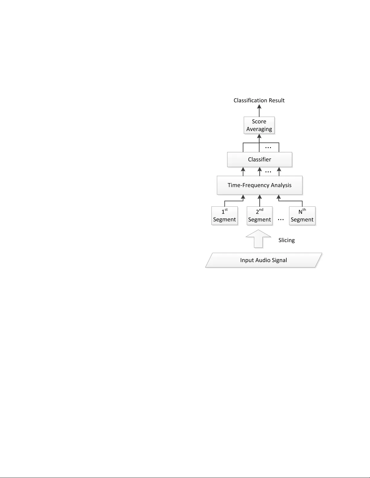
IEEE Copyright Notice c  2018 IEEE. Personal use of this material is permitted. Permission from IEEE must be obtained for all other uses, in any current or future media, including reprinting/republishing this ma- terial for advertising or promotional purposes, creating new collectiv e works, for resale or redistrib ution to servers or lists, or reuse of any cop yrighted component of this work in other works. Accepted by 2018 IEEE International Conference on Acoustics, Speech and Signal Pro- cessing (ICASSP 2018), 15-20 April 2018, Calgary , Alberta, Canada Full citation: Y . W u and T . Lee, ”Reducing Model Complexity for DNN Based Lar ge-Scale Audio Classification, ” 2018 IEEE International Conference on Acoustics, Speech and Signal Processing (ICASSP), Calgary , AB, 2018, pp. 331-335. Link in IEEE Xplore: https://ieeexplore.ieee.or g/document/8462168 REDUCING MODEL COMPLEXITY FOR DNN B ASED LARGE-SCALE A UDIO CLASSIFICA TION Y uzhong W u, T an Lee Department of Electronic Engineering, The Chinese Uni versity of Hong K ong ABSTRA CT Audio classification is the task of identifying the sound categories that are associated with a given audio signal. This paper presents an in vestigation on lar ge-scale audio classification based on the re- cently released AudioSet database. AudioSet comprises 2 millions of audio samples from Y ouT ube, which are human-annotated with 527 sound category labels. Audio classification experiments with the balanced training set and the ev aluation set of AudioSet are car- ried out by applying dif ferent types of neural network models. The classification performance and the model complexity of these mod- els are compared and analyzed. While the CNN models show better performance than MLP and RNN, its model comple xity is relati vely high and undesirable for practical use. W e propose two different strategies that aim at constructing lo w-dimensional embedding fea- ture extractors and hence reducing the number of model parameters. It is shown that the simplified CNN model has only 1 / 22 model parameters of the original model, with only a slight degradation of performance. Index T erms — Audio classification, DNN, embedding features, reducing model complexity 1. INTR ODUCTION The rapid dev elopment of technology has made the production, ren- dering, sharing and transmission of multimedia data easy , low-cost and hence become part of our daily life. The growth of online av ail- able (public or restricted-access) audio and visual data is irre versible trend. Having effecti ve and efficient tools for classifying, indexing and managing multimedia data is not only for the conv enience and enjoyment of indi viduals, b ut also critical to the social and economic dev elopment in the big data era. Audio is inar guably one of the most important types of multi- media resources to be reckoned. Audio classification is generally defined as the task of identifying a given audio signal from one of the predefined categories of sounds. Depending on the applications, the sound categories could be broad, e.g., music, v oice, noise, or highly specified, e.g., children speech. The existence of di verse task definitions has made it difficult to compare the methods and results from different research groups and therefore hindered constructiv e exchange of ideas. In recent years, there hav e been or ganised ef forts on setting up open ev aluation or competitions on large-scale audio classification. For example, the IEEE AASP challenge DCASE2016 includes the acoustic scene classification (ASC) as an important part. The ASC task is to classify a 30 -second audio sample as one of the 15 pre-defined acoustic scenes. Among the 30 participating teams in DCASE2016 ASC, Eghbal-Zadeh et al. [1] proposed a hybrid model using binaural I-vectors and CNN, and demonstrated the best perfor - mance. It was shown that log-mel filterbank features perform better than MFCC, when CNN models are applied [2]. In DCASE2017, CNN is most popular among the top- 10 models. Mun et al. [3] addressed the problem of data insuf ficiency and proposed to apply GAN-based data augmentation method to significantly improve the classification accuracy . There was also a trend on using binaural audio features rather than monaural features. The DCASE2016 ASC task provides an annotated database that contains 9 . 75 hours of audio recordings for training. Such an amount is considered inadequate to exploit the full capability of the latest deep learning techniques. In ICASSP 2017, the Sound and V ideo Understanding team at Google Research announced the release of AudioSet [4], which comprises a lar ge amount of audio samples from Y ouTube. The total duration of data in the current release of AudioSet exceeds 5000 hours. Unlike the DCASE2016 ASC database, audio samples in AudioSet are labeled by a large number of sound categories which are or ganised in a loose hierarchy . While the availability of AudioSet has caught great attention from the re- search community , there ha ve been fe w published studies that report referable classification performance on the database. In [5], a related database named Y ouT ube-100M was used to in vestigate large-scale audio classification problem. The Y ouT ube-100M dataset contains 100 million Y ouTube videos. The experimental results show that with massiv e amount of training data, a residual network with 50 layers produces the best performance, in comparison with the MLP , AlexNet, V GG and Inception network [5]. This paper presents our recent attempt to large-scale audio clas- sification with the newly released AudioSet. T o our knowledge, ex- cept for the preliminary e valuation briefly mentioned in [5], there has been no official published result on the complete AudioSet clas- sification task. W e apply a variety of commonly used DNN mod- els on the AudioSet task and find that CNN based models generally achiev e better performance than MLP and RNN. W e further propose to exploit low-dimension feature representation of audio segments, so as to achiev e significant reduction of CNN model complexity . It is shown that the number of model parameters could be reduced by 22 times while maintaining comparable performance of classification. In addition, the effecti veness of the proposed methods is validated on the DCASE2016 ASC database. In Section 2, the AudioSet and the TUT Acoustic Scenes 2016 database are described. The general frame work of the classification system and the proposed strategy of model complexity reduction are explained in Section 3. Experimental results with dif ferent types of neural network models are gi ven in Section 4. 2. D A T ASETS FOR A UDIO CLASSIFICA TION 2.1. A udioSet The AudioSet is a large-scale collection of human-annotated au- dio segments from Y ouT ube [4]. It is provided as text (csv) files that contain the following attrib utes of each audio sample: Y ouT ube V ideo ID, start time and end time of the audio clip, and sound cat- egory labels. Each audio clip is 10 second long. The sound labels were obtained through a human-annotation process, in which human raters were asked to confirm the presence of a set of hypothesized sound categories. Both audio and video components were presented to the raters. The hypothesized sound categories were generated from multiple sources, including a video-labeling system and v ar- ious meta-data information. There may be multiple sound categories co-existing in an audio clip. There are totally 527 sound categories being used in AudioSet. These categories are arranged following a loose hierarchy . For example, “speech” and “male speech” are treated as two categories at different hierarchical levels. Howe ver , this kind of hierarchy is not taken into account in the audio classifi- cation experiments. The entire AudioSet contains about 2 million audio samples, which correspond to more than 5 , 000 hours of data. The audio samples are divided into the balanced training set, the unbalanced training set and the ev aluation set. In this study , only the balanced training set and ev aluation set are used. A number of audio sam- ples are excluded for various reasons, e.g., deleted Y ouT ube links, duration shorter than 10 seconds. As a result, the number of audio samples used for training and e valuation are 20 , 175 and 18 , 396 re- spectiv ely . A validation set is created by randomly selecting 10% of the training data. 2.2. TUT Acoustic Scenes 2016 database The TUT Acoustic Scenes 2016 database [6] was used in the DCASE2016 challenge. There are 15 defined acoustic scenes, cov ering various indoor and outdoor en vironments. The develop- ment dataset contains 1170 audio samples and the e valuation dataset contains 390 samples. The number of samples representing different scene classes are the same. Each audio sample is 30 second long and said to be from one and only one of the 15 scenes. The total duration of recordings is 13 hours. 3. SYSTEM DESIGN 3.1. General System Framework Figure 1 shows the general framework of a segment-based audio classification system. The typical length of a segment is 1 second. A segment can be di vided into short-time frames (typically 25 ms long) which are used for spectral analysis. The segment-based system can make better use of the temporal information of audio signals than the frame-based system (e.g., the baseline GMM model in DCASE2016 ASC task [7]). In Figure 1, the input audio signal (e.g., 10 -second audio clip in AudioSet) is divided into non-overlapping segments. The sound category labels of a se gment are inherited from those of the input audio signal. For each se gment, a time-frequency repre- sentation is deriv ed for classification purpose. The time-frequency features of each segment are fed into a classifier to obtain the clas- sification scores. The sample-level classification score is calculated by av eraging the segment-le vel scores. Commonly used time-frequency representations for audio clas- sifications are derived from the short-time Fourier transforms. Ex- amples include log-mel filterbank features, Constant-Q transform (CQT) [8], and MFCC. Based on our preliminary experiments, for DNN-based systems, the log-mel features gi ve the best performance among these feature types, and thus are used in our experiments. For the classifier in Figure 1, our main focus of experiments is the DNN models. There has been gro wing interest in extracting the embedding features from a well-trained DNN classifier in audio clas- sification area. For example, Rakib et al. [9] uses the trained CNN model to extract its embedding feature, which is fed into PLDA to improv e classification performance. In [3], the use of embedding features from a trained DNN classifier also serve as a critical com- ponent in its proposed method. In this paper , sev eral ways to obtain low-dimensional embedding feature are studied in Section 4.3. Fig. 1 : The general frame work for a segment-based audio classifica- tion system. 3.2. Strategy for Reducing Model Complexity 3.2.1. Use of Bottleneck Layer Bottleneck layer has been applied in speech recognition area to ex- tract embedding features. The extracted feature is called bottleneck feature and is generally better than the hand-crafted feature [10]. Re- cently , bottleneck layers were inv estigated in large-scale audio clas- sification by Shawn Hershey et al. [5]. The introduction of bot- tleneck layer leads to faster training, while maintaining comparable classification performance. A bottleneck layer typically lies in between two (hidden) layers in a fully-connected neural network. It is a middle layer designed to hav e a relativ ely small number of neurons as compared to other hidden layers, and therefore called “bottleneck”. By constructing a bottleneck layer , a low-dimensional feature representation of input data can be generated. Figure 2 shows an example of MLP with a bottleneck layer . In this study , we make use of the bottleneck layers to achieve reduction of model comple xity , and through which low-dimensional embedding feature extractor is constructed. Different sizes of bottle- neck layer are experimented to rev eal the trade-off between model performance and complexity . Fig. 2 : An illustration of bottleneck layer in a multi-layer perceptron (MLP). The bottleneck layer has smaller size than its adjacent layers. 3.2.2. Global A vera ge P ooling A CNN-based classification model is typically composed of con vo- lution layer(s) and fully connected (FC) layer(s). The common way of making connection between a conv olution layer and a FC layer is by flattening (v ectorizing) the feature maps of the con v olutional layer and using the flattened features as the input of the FC layer . Since the flattened features ha ve a v ery large dimension, the number of required model parameters w ould be excessi ve. Moreover , it may increase the chance of ov er-fitting of the FC layers. In [11], global average pooling strategy is proposed to solve the problem of over -fitting of FC layers, and its effecti veness of being a regularizer has been verified. It is an av erage pooling operation ap- plied on each feature map obtained from the last con volutional layer, with the size of pooling window equal to the size of feature map. This pooling result is used as the input of FC layer(s) for classifi- cation. Figure 3 illustrates the con ventional way and global average pooling to transform 2D feature maps into 1D feature vector . In this study , we emphasize global average pooling for its effi- cacy of reducing CNN model complexity , while preserving the per- formance of classification. Fig. 3 : Left: con ventional w ay of linking up con volutional layer and fully connected layer; right: global average pooling. 4. EXPERIMENTS 4.1. EXPERIMENT AL SETUP 4.1.1. Data Pr epr ocessing Each audio sample in the dataset is divided into non-overlapping 1 -second se gments. The sound category labels assigned to each seg- ment are exactly the same as the source audio sample. Short-Time Fourier T ransform (STFT) is applied on the audio segments with a window length of 25 ms, hop length of 10 ms and FFT length of 2048 . Subsequently 64 -dimensional log-mel filterbank features are deriv ed from each short-time frame, and the frame-le vel features are put together to form a time-frequenc y matrix representation of the segment. Dimension-wise normalization of the log-mel features is performed using the means and variances calculated from all audio samples in the training set. 4.1.2. P erformance Metric The Area Under Recei ver Operating Characteristic curve, abbrevi- ated as A UC [12], is used as our performance metric in the exper- iments with the AudioSet. In the context of binary classification, A UC can be viewed as the probability that the classifier ranks a ran- domly chosen pos itive sample higher than a negati ve one [13]. For a classification model only makes random guesses, the A UC value is 0 . 5 . A perfect classification model giv es the A UC value of 1 . 0 . A UC is found to be insensitive to the distribution of positive and negati ve samples, as compared to other ev aluation metrics like precision, ac- curacy , F 1 score and mAP . For a multi-class problem, the o verall measure of A UC is ob- tained as the weighted av erage of the A UC values for individual classes. The weight for a specific class is proportional to its prev a- lence in the dataset. 4.1.3. Model T raining and P arameter Setting The experimented models in this study are implemented using the deep learning toolbox PyT orch (http://pytorch.or g/). The key pa- rameters used for training are empirically determined. The initial learning rate and mini-batch size are set to 0 . 0001 and 60 . Model training is done by minimizing the cross-entropy loss with the Adam optimizer ( β 1 = 0 . 9 and β 2 = 0 . 999 ) and learning rate decay strat- egy . For MLP and CNN models, dropout (with dropout probability = 0 . 5 ) and weight decay (coef ficient = 0 . 0015 ) are applied for re g- ularization purpose. The sigmoid function is used in the output layer for all models, considering that an audio sample may have multiple sound labels. 4.2. Model Comparison T able 1 shows the experimental results with six different models (or different model configurations). The MLP model has 3 hidden layers with 1000 neurons per layer . For the MLP , batch normalization and the ReLU activ ation function are applied. The LSTM (Long-Short T erm Memory) model contains 3 LSTM layers, each having 2048 units. GRU refers to Gated Recurrent Unit [14]. B-GR U-A TT refers to bi-directional GR U with its output weighted by attention network [15] whose context vector size is 1024 . It has 2 GRU layers, each with 2048 units. T o our knowledge, performance of recurrent mod- els has not been reported for AudioSet yet. CNN models have been in vestigated for large-scale audio clas- sification on Y ouT ube-100M database in [5]. In this study , the CNN models being experimented are the AlexNet and Residual Network with 50 layers (ResNet-50) [16]. The AlexNet used in our exper - iments is similar to the AlexNet described in [17], which was de- signed for image classification with 224 × 224 × 3 input. W e make a change of its first con volutional layer to ha ve a kernel size of 11 × 7 and stride of 2 × 1 , so as to obtain a similar size of feature map at the first conv olutional layer . For the FC layers, the size is set to 3982 . By Ale xNet(BN), we mean that a batch normalization layer is added after each layer (con volutional and FC). For the ResNet- 50 model, we follow the same setting as in [5], by changing the stride to 1 in the first conv olution layer . As a result, the windo w length of its global a verage pooling layer is set to 7 × 4 , T able 1 : Classification performance of six DNN models tested on AudioSet evaluation set, trained with the balanced training set. The letter “M” in “Model Size” column stands for million. Model Structure Model Size A UC MLP 3 × 1000 9 . 48 M 0 . 845 LSTM 3 × 2048 85 . 54 M 0 . 866 B-GR U-A TT 2 × 2048 107 . 85 M 0 . 870 AlexNet - 56 . 09 M 0 . 895 AlexNet(BN) - 56 . 11 M 0 . 927 ResNet-50 - 24 . 58 M 0 . 914 to match the change of feature map size. The model sizes given in the table refer to the number of model parameters in the respectiv e models. The overall A UC is calculated over 527 audio classes (see Sec- tion 4.1.2). It can be seen that the AlexNet with batch normaliza- tion performs the best among all tested models. It even outperforms the 50 -layer deep residual network, which was reported to hav e the highest performance among CNN models for lar ge-scale audio clas- sification [5]. 4.3. Reducing Model Complexity While the AlexNet(BN) model has been sho wn to ha ve the best per - formance among different DNN models, its model complexity is rel- ativ ely lar ge and thus undesirable for practical use. As described in Section 3.2, using a bottleneck layer and performing global average pooling are ef fectiv e techniques of reducing the number of model parameters. W e experiment with different arrangements of the FC layers and the bottleneck layer in the AlexNet(BN) model. The re- sults are compared as in T able 2. “Bneck-Final-64” refers to that a 64 -dimension bottleneck layer is inserted between the output layer and the last FC layer , while “Bneck-Mid-64” means that the 64 - dimension bottleneck layer is inserted between the two FC layers. For the “FC-64” configuration, the size of both FC layers is reduced to 64 . Three different sizes of embedding features are tested: 64 , 256 and 1024 . Lastly , “Global-avg-pool” means that a global a ver- age pooling layer is used to replace the two FC layers. The resulting feature dimension after pooling is 256 , which is equal to the number of feature maps in the last con volution layer . Generally , a larger size of bottleneck layer or FC layers lead to better classification performance. Reducing the size of existing FC layers without having an additional bottleneck layer would cause noticeable degradation of performance, despite the significantly re- duced model complexity . With the same size of bottleneck layer , it is more beneficial to hav e the bottleneck inserted between the two FC layers (i.e., the “Bneck-Mid” configurations). “Bneck-Mid- 1024 ” could attain the same A UC as the original AlexNet(BN), with about 14% less model parameters. By applying global av erage pooling strategy , the model complexity is reduced to 2 . 59 M. which is about 1 / 22 of the original AlexNet(BN), 1 / 9 of the ResNet- 50 model, and 1 / 4 of the MLP model. Its performance is comparable to the ResNet- 50 model, and slightly worse than the AlexNet(BN). 4.4. Acoustic Scene Classification in DCASE2016 The proposed models are also ev aluated with the TUT Acoustic Scenes 2016 database. Due to the different nature of the scene clas- sification task, softmax function is used at the output layers of the neural networks. The other settings of training are the same as stated T able 2 : Performance of 4 types of strategies for reducing model complexity . All strategies are applied on the same AlexNet(BN) model as described in Section 4.2. Strategy Model Size A UC None 56 . 11 M 0 . 927 Bneck-Final- 64 54 . 30 M 0 . 889 Bneck-Final- 256 55 . 17 M 0 . 917 Bneck-Final- 1024 58 . 63 M 0 . 925 Bneck-Mid- 64 40 . 77 M 0 . 915 Bneck-Mid- 256 42 . 29 M 0 . 924 Bneck-Mid- 1024 48 . 41 M 0 . 927 FC- 64 3 . 07 M 0 . 841 FC- 256 4 . 95 M 0 . 905 FC- 1024 13 . 22 M 0 . 924 Global-avg-pool 2 . 59 M 0 . 916 in Section 4.1.3. Among the 1170 audio samples in the training set, 170 samples are randomly selected to be the validation data. The AlexNet(BN) model attains a classification accuracy of 87 . 4% on the ev aluation set, while a 3 -layer MLP with 1000 neurons per layer has an accuracy of 78 . 2% , and a well-tuned LSTM model has an accuracy of 82 . 8% . By applying the strategy of global average pooling, the size-reduced AlexNet(BN) has an accuracy of 85 . 9% . This further confirms the effecti veness of CNN and global average pooling strate gy , though the ASC may not be vie wed as a lar ge-scale task as compared to the AudioSet. 5. CONCLUSION The AudioSet database provides useful resources to enable and advance research on large-scale audio classification. This paper presents one of the earliest batches of experimental results on this database using the latest neural network models. It has been shown that CNN models are more ef fecti ve than MLP and RNN. The model complexity of the best-performing CNN can be significantly reduced by introducing a bottleneck layer at the fully-connected layers and by applying global av erage pooling. It must be noted that only a small portion of AudioSet has been used in the present study , though this small portion already contains 20 times more audio samples than the existing DCASE2016 ASC database. 6. REFERENCES [1] H. Eghbal-Zadeh, B. Lehner , M. Dorfer , and G. W idmer , “CP- JKU submissions for DCASE-2016: a hybrid approach using binaural i-vectors and deep con volutional neural netw orks, ” T ech. Rep., DCASE2016 Challenge, September 2016. [2] M. V alenti, A. Diment, G. Parascandolo, S. Squartini, and T . V irtanen, “DCASE 2016 acoustic scene classification us- ing con volutiona l neural networks, ” T ech. Rep., DCASE2016 Challenge, September 2016. [3] S. Mun, S. Park, D. Han, and H. Ko, “Generativ e adversar - ial netw ork based acoustic scene training set augmentation and selection using SVM hyper-plane, ” T ech. Rep., DCASE2017 Challenge, September 2017. [4] J. F . Gemmeke, D. P . W . Ellis, D. Freedman, A. Jansen, W . Lawrence, R. C. Moore, M. Plakal, and M. Ritter , “ Audio set: An ontology and human-labeled dataset for audio e vents, ” in Pr oc. IEEE ICASSP 2017 , New Orleans, LA, 2017. [5] S. Hershey , S. Chaudhuri, D. P . W . Ellis, J. F . Gemmeke, A. Jansen, R. C. Moore, M. Plakal, D. Platt, R. A. Saurous, B. Seybold, M. Slaney , R. J. W eiss, and K. W ilson, “CNN ar- chitectures for lar ge-scale audio classification, ” in Pr oc. IEEE ICASSP 2017 , New Orleans, LA, 2017. [6] A. Mesaros, T . Heittola, and T . V irtanen, “T ut database for acoustic scene classification and sound event detection, ” in Sig- nal Pr ocessing Conference (EUSIPCO), 2016 24th Eur opean . IEEE, 2016, pp. 1128–1132. [7] T . Heittola, A. Mesaros, and T . V irtanen, “DCASE2016 base- line system, ” T ech. Rep., DCASE2016 Challenge, September 2016. [8] J. C. Bro wn, “Calculation of a constant Q spectral transform, ” Acoustical Society of America Journal , vol. 89, pp. 425–434, Jan. 1991. [9] R. Hyder, S. Ghaffarzade gan, Z. Feng, J. H. L. Hansen, and T . Hasan, “ Acoustic scene classification using a cnn- supervector system trained with auditory and spectrogram im- age features, ” in Pr oc. INTERSPEECH 2017 , Stockholm, Swe- den, 2017. [10] J. Gehring, Y . Miao, F . Metze, and A. W aibel, “Extracting deep bottleneck features using stacked auto-encoders, ” in 2013 IEEE International Conference on Acoustics, Speech and Sig- nal Pr ocessing , May 2013, pp. 3377–3381. [11] M. Lin, Q. Chen, and S. Y an, “Network In Network, ” ArXiv e-prints , Dec. 2013. [12] M. V uk and T . Curk, “ROC Curve, Lift Chart and Calibration Plot, ” Metodoloski zvezki , vol. 3, no. 1, pp. 89–108, 2006. [13] T . Fa wcett, “ An introduction to roc analysis, ” P attern Recogni- tion Letters , v ol. 27, no. 8, pp. 861 – 874, 2006, ROC Analysis in Pattern Recognition. [14] J. Chung, C. Gulcehre, K. Cho, and Y . Bengio, “Empirical Evaluation of Gated Recurrent Neural Networks on Sequence Modeling, ” ArXiv e-prints , Dec. 2014. [15] Z. Y ang, D. Y ang, C. Dyer , X. He, A. J. Smola, and E. H. Ho vy , “Hierarchical attention networks for document classification, ” in Pr oc. NAA CL-HLT , 2016. [16] K. He, X. Zhang, S. Ren, and J. Sun, “Deep Residual Learning for Image Recognition, ” ArXiv e-prints , Dec. 2015. [17] A. Krizhevsky, “One weird trick for parallelizing conv olu- tional neural networks, ” ArXiv e-prints , Apr . 2014.