Robust Learning of Fixed-Structure Bayesian Networks

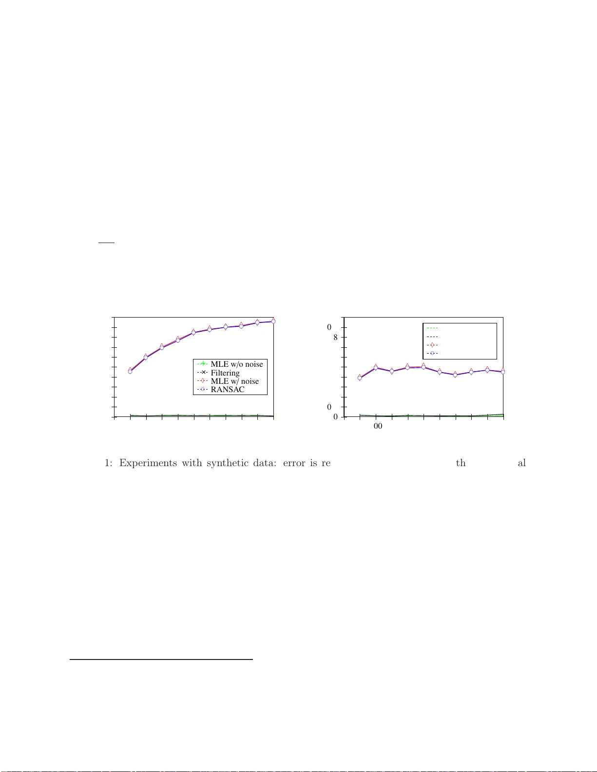
Robust Learning of Fixed-Structure Ba y esian Net w orks Y u Cheng Duk e Unive rsit y yucheng@c s.duke.ed u Ilias Diak onik olas Univ ersit y of Southern California ilias.dia konikolas @gmail.com Daniel M. Kane Univ ersit y of California, San Diego dakane@uc sd.edu Alistair Stew art Univ ersit y of Southern California stewart.a l@gmail.c om Octob er 30, 2018 Abstract W e inv estiga te the problem of learning Bayesian net works in a robust mo del where an ǫ - fraction of the samples are adversarially corrupted. In this w ork, we study the fully observ able discrete case where the structure of the netw ork is g iven. Even in this basic setting, prev io us learning algor ithms either run in exp onential time or lose dimension-dep endent factors in their error guarantees. W e provide the ﬁr st co mputationally eﬃcient r obust lear ning algor ithm for this problem with dimension- independent error g uarantees. Our algor ithm has near-o ptimal sample c omplexit y , runs in po lynomial time, and a c hieves error that scales nearly-linea r ly with the fractio n of adversaria lly co rrupted samples. Finally , we show on bo th synthetic and semi- synthet ic data that our a lgorithm p erforms well in practice. 1 In tro duction Probabilistic graphical mo dels [KF09] pro vide an app ealing and unifying f ormalism to succinctly represen t structured high-dimension al distributions. The general problem of inference in graphi- cal mo dels is of fundamen tal imp ortance and arises in man y ap plications across sev eral scien tiﬁc disciplines, see [WJ08] and references therein. In this w ork, w e s tudy the problem of learning graphical mo dels from data [Nea03, DSA11 ]. There are sev eral v arian ts of this general learning problem dep ending on: (i) the precise family of graphical mo dels considered (e.g., direct ed, undi- rected), (ii) whether the data is fully or partially observ able, and (iii) whether the structure of the underlying graph is kno wn a priori or not (parameter estimation versus structure learning). This learning problem has b een studied extensiv ely along these axes during the past ﬁv e decades, (see, e.g., [CL68, Das97, AKN06, WRL06, AHHK12, SW12, L W12, BMS13, BGS14, Bre15]) resulting in a b eautiful theory and a collection of algorithms in v arious settings. The main vulnerabil it y of all these algorithmic tec hniques is that they crucially rely on the assumption that the samples are precisely generated b y a graphical mo del in the giv en family . This simplifying ass umption is inheren t for k no wn guaran tees in the follo wing sense: if there exists ev en a very small fraction of arbitrary outliers in the dataset, the p erformance of kno wn algorithms can b e totally compromised. It is imp ortan t to explore the natural setting when the aforemen tioned assumption holds only in an appro ximate sense. Sp eciﬁcally , we study the follo wing broad question: 1 Question 1 (Robust Learning of Graphical Mo dels) . Can we eﬃciently le arn gr aphic al mo dels when a c onstant fr action of the samples ar e c orrupte d, or e quivalently, when the mo del is sli ghtly missp e ciﬁe d? In this p ap er, w e fo cus on the mo del of corruptions considered in [DKK + 16] (Deﬁnition 1) which generalizes man y other existing mo dels, including Hub er’s con tamination mo del [Hub64]. Intu itiv ely , giv en a set of go o d samples (from the true mo del), an adversary is allo w ed to insp ect the samples b efore corrupting them, both by adding corrupted p oint s and deleting go o d samples. In cont rast, in H ub er’s mo del, the adv ersary is oblivious to the s amples and is only allo wed to add bad p oin ts. W e wo uld like to design robust learning algorithms for Quest ion 1 whose sample complexit y , N , is close to the information-theo retic minim um, and whose co mputatio nal complexit y is p olynomial in N . W e emphasize that the crucial requiremen t is that the error guaran tee of the algorithm is indep endent of the dimensionalit y d of the problem. 1.1 F ormal Setting and Our Results In this w ork, w e study Question 1 in the con text of Bayesian networks [JN07]. W e fo cus on the fully observ able case when the underlying net w ork is given. In the non-r obust s etting, this learning problem is straigh tforwar d: the “empirical estimator” (whic h coincides with the maximu m likelihoo d estimator) is kno wn to b e sample and computationall y eﬃcien t [Das97]. I n sharp con trast, even this most basic regime is surprisingly ch allenging in the robust setting. F or example, the v ery sp ecial case of robustly learning a Bernoulli pro duct distribution (corresp onding to an empt y netw ork with no edges) was analyzed only recen tly in [DKK + 16]. T o formally state our results, w e ﬁrst giv e a detailed description of the corruption mo del w e study . Deﬁnition 1 ( ǫ -Corrupted Samples) . Given 0 < ǫ < 1 / 2 and a distri bution f amily P , the algo- rithm sp e ciﬁes some numb er of samples N , and N samples X 1 , X 2 , . . . , X N ar e dr awn fr om some (unknown) gr ound-truth P ∈ P . T he adversary is al lowe d to insp e ct P and the samples, an d r eplac es ǫN of them with arbitr ary p oints. The set of N p oints is then given to the algorithm. W e say that a set of samples is ǫ -c orrupte d if it is gener ate d by this pr o c ess. Ba yesia n Net w ork s. Fix a dire cted acyclic graph, G , whose v ertices are lab elled [ d ] def = { 1 , 2 , . . . , d } in top ological order (ev ery edge p oin ts from a ve rtex with a s maller index to one with a larger index). W e will denote b y P arents ( i ) the set of paren ts of no de i in G . A probabilit y distribution P on { 0 , 1 } d is deﬁned to b e a Bayesian n etwork (or Bayes net ) with graph G if f or each i ∈ [ d ] , w e ha ve that Pr X ∼ P [ X i = 1 | X 1 , . . . , X i − 1 ] depends only on the v alues X j where j ∈ P aren ts ( i ) . Suc h a distribution P can b e sp eciﬁed by its c onditional pr ob ability table . Deﬁnition 2 (Condition al Probabilit y T able of Bay esian Net wor ks) . L et P b e a Bayesian network with gr aph G . L et Γ b e the s et { ( i, a ) : i ∈ [ d ] , a ∈ { 0 , 1 } | Paren ts ( i ) | } . L et m = | Γ | . F or ( i, a ) ∈ Γ , the paren tal conﬁguration Π i,a is deﬁne d to b e the event that X Pa rent s( i ) = a . The c onditional pr ob ability table p ∈ [0 , 1] m of P i s given by p i,a = Pr X ∼ P [ X i = 1 | Π i,a ] . Note that P is determined b y G and p . W e will frequen tly index p as a vector. W e use the nota- tion p k and the asso ciated even ts Π k , where each k ∈ [ m ] s tands for an ( i, a ) ∈ Γ lexicographically ordered. 2 Our Results. W e giv e the ﬁrst eﬃcien t robust learning algorithm for Bay esian netw orks with a kno wn graph G . Our algorith m has information- theoretically near-optimal sample complexit y , runs in time p olynomial in the size of the input (the samples), and pro vides an error guaran tee that scales near-linearly with the fraction of adv ersarially corrupted samples, under the follo wing restrictions: First, w e assume that eac h paren tal conﬁguration is reasonably likel y . In tuitively , this assumption seems necessary b ecause we need to observ e eac h conﬁguration man y times in order to learn the asso ciated conditional probabilit y to goo d accuracy . Second, w e assume that eac h of the conditional probabi lities is balanced, i.e., b ounded a w ay from 0 and 1 . This as sumption is needed for techn ical reasons. In particular, we need this to sho w that a go o d appro ximation to the conditional probabilit y table implies that the corresp onding Bay esian net w ork is close in total v ariation distance. F ormally , w e sa y that a Ba y esian netw ork is c -b alanc e d , for some c > 0 , if all co ordinates of the corresp onding conditional probabilit y table are b etw een c and 1 − c . Throughout the pap er, w e use m = P d i =1 2 | Paren ts( i ) | for the size of the conditional probabilit y table of P , and α for the minim um probabilit y of paren tal conﬁguration of P : α = min ( i,a ) ∈ S Pr P [Π i,a ] . W e now state our main result. Theorem 3 (Main) . Fix 0 < ǫ < 1 / 2 . L et P b e a c -b alanc e d Bayesian n etwork on { 0 , 1 } d with known structur e G . Assume α ≥ Ω( ǫ p log(1 /ǫ ) /c ) . L et S b e an ǫ -c orrupte d set of N = e Ω( m log (1 /τ ) /ǫ 2 ) samples fr om P . 1 Given G, ǫ, τ , and S , we c an c ompute a Bayesian network Q such that, with pr ob ability at le ast 1 − τ , d T V ( P , Q ) ≤ ǫ p ln(1 /ǫ ) / ( αc ) . Our algorithm runs in ti me e O ( N d 2 /ǫ ) . Our algorithm is giv en in Section 3 . W e ﬁrst note that the s ample complexit y of our algorithm is near-optima l for learning Ba y es ian net wo rks with k no wn structure. The follo wing sample complexit y lo wer b ound holds ev en without corrupted samples: F act 4 (Sample Complexit y Lo wer Bound, [CDKS17]) . L et B N d,f denote the family of Bernoul li Bayesian networks on d variables such that every no de has at m ost f p ar ents. T he worst-c ase sample c om plexity of le arning B N d,f , wi thin total variation dis tanc e ǫ and with pr ob ability 9 / 10 , is Ω(2 f · d/ǫ 2 ) for al l f ≤ d/ 2 when the gr aph structur e is known. Consider Bay es nets whose a v erage in-degree is close to the maxim um in-degree, that is, when m = Θ (2 f d ) , the s ample complexit y lo w er b ound in F act 4 becomes Ω( m/ǫ 2 ) , so our s ample complexit y is optimal up to p olylogarithmic factors. W e remark that Theorem 3 is most useful when c is a constan t and the Bay esian net work has b ounded fan-in f . In this case, the condition on α follows from the c -balanced assumption: When b oth c and f are constan ts, α = min ( i,a ) ∈ S Pr P [Π i,a ] ≥ c f is also a constan t, so the condition c f ≥ Ω( ǫ p log(1 /ǫ )) automatically hold when ǫ is smaller than some constan t. On the other hand, the problem of learning Ba yesian net w orks is less in teresting when the fan-in is too large. F or example, if s ome no de has f = ω (log( d )) paren ts, then the size of the conditional probabilit y table is at least 2 f , whic h is sup er-p olynomial in the dimension d . Exp erimen ts. W e p erformed an exp erimen tal ev aluation of our algorithm on b oth synth etic and real data. Our ev aluation allo w ed us to verify the accuracy and the sample complexit y rates of our theoretical results. In all cases, the exp erimen ts v alidate the usefulness of our algorithm, whic h signiﬁcan tly outp erforms previous approac hes, almost exactly matc hing the b est rate without noise. 1 Throughout the pap er, we use e O ( f ) t o den ote O ( f p olylog( f ) ) . 3 Related W ork. Question 1 ﬁts in the framew ork of robust s tatistics [HR09, HRRS86]. Classical estimators f rom this ﬁeld can b e classiﬁed in to t w o categories: either (i) they are computationally eﬃcien t but incur an error that scales p olynomial ly with the dimension d , or (ii) they are pro v ably robust (in the aforemen tioned sense) but are hard to compute. In particular, essent ially all known estimators in robust statistics (e.g., the T uk ey median [T uk75]) hav e b een sho wn [JP78, Ber06, HM13] to b e in tractable in the high-dimensional s etting. W e note that the robustness requiremen t do es not typically p ose inf ormation-theoretic impedimen ts for the learning problem. I n most cases of in terest (see, e.g., [CGR15, CGR16, DKK + 16]), the sample complexit y of robust learning is comparable to its (easier) non-robust v arian t. The c hallenge is to design c omputational ly eﬃcient algorithms. Eﬃcien t robust estimators are known for v arious low-dimensional structured distributions (see, e.g., [DDS14, CDSS13, CDSS14a, CDSS14b, ADLS16, ADLS17, DL S18]). H o w ev er, the robust learning problem b ecomes surprisingly ch allenging in high dimensions. Recen tly , there has b een algorithmic progress on this fron t: [DKK + 16, LR V16] give p olynomial-time algorithm s with im- pro ved error guaran tees for certain “simple” high-dimensional s tructured distributions. The results of [DKK + 16] apply to s imple distributions, including Bernoulli pro d uct distributions, Gaussians, and mixtures thereof (under s ome natural restrictions). Since the works of [DKK + 16, LR V16], com- putationally eﬃcien t robust estimation in high dimensions has receiv ed considerable atten tion (see, e.g., [DKS17, DKK + 17, BDLS17, DKK + 18a, DKS18b, DKS18a, HL18, KSS18, PSBR18, DKK + 18b, KKM18, DKS18c, LSLC18]). 1.2 Ov erview of Algorithmic T ec hniques Our algorithmic approac h builds on the framew ork of [DKK + 16] with new techn ical and conceptual ideas. At a high lev el, our algorithm w orks as follo ws: W e draw an ǫ -corrupted set of samples from a Ba yesian net w ork P with kno wn structure, and then iteratively remo ve samples until w e can return the empirical conditional probabilit y table. First, w e asso ciate a vec tor F ( X ) to each sample X so that learning the mean of F ( X ) to go o d accuracy is suﬃcien t to reco ver the distribution. In the case of binary pro ducts, F ( X ) is simply X , while in our case w e need to tak e in to accoun t additional information ab out conditiona l means. F rom this p oint, our algorithm will try to do one of t w o things: Either w e sho w that the sample mean of F ( X ) is close to the conditional mean of the true distribution (in which case w e can already learn the ground-truth Ba yes net P ), or we are able to pro duce a ﬁlter , i.e., w e can remo v e some of our samples, and it is guaran teed that w e thro w a w ay more bad samples than go od ones. If w e pro duce a ﬁlter, we then iterate on those samples that pass the ﬁlter. T o produce a ﬁlter, w e compute a matrix M whic h is roughly the empirical cov arian ce matrix of F ( X ) . W e sho w that if the corruptions are suﬃcien t to notably disrupt the s ample mean of F ( X ) , there m ust b e man y erroneous s amples that are all f ar from the mean in roughly the same direction, and w e can detect this direction by lo oking at the largest eigen vect or of M . If we pro ject all samples onto this direction, concen tration b ounds of F ( X ) will imply that almost all samples far from the mean are erroneous, and th us ﬁltering them out will pro v ide a cleaner s et of samples. Organization. Section 2 con tains some tec hnical results s p eciﬁc to Ba yesian net works that we need. Section 3 give s the details of our algorithm and an o verview of its analysis. In Section 4, w e presen t the exp erimen tal ev aluations. In Section 5 , w e conclude and prop ose directions for future w ork. 4 2 T ec hnical Preli minaries The s tructure of this s ection is as follows: First, we b ound the total v ariation distance b et w een t w o Ba yes nets in terms of their condition al probabilit y tables. Second, w e deﬁne a function F ( x, q ) , whic h takes a sample x and returns an m -dimensional vector that con tains information ab out the conditional means. Finally , w e deriv e a concen tration b ound from Azuma’s inequalit y . Proofs f rom this s ection hav e b een deferred to App endix A . Lemma 5. Supp ose that: (i) m in k ∈ [ m ] Pr P [Π k ] ≥ ǫ , and (ii) P or Q is c -b alanc e d, and (iii) 3 c p P k Pr P [Π k ]( p k − q k ) 2 ≤ ǫ . Then we have that d T V ( P , Q ) ≤ ǫ. Lemma 5 sa ys that to learn a balanced ﬁxed-structure Ba y esian net w ork, it is suﬃcien t to learn all the relev ant conditional means. How ev er, eac h sample x ∼ P giv es us information about p i,a only if x ∈ Π i,a . T o resolv e this, w e map each sample x to an m -dimen sional v ector F ( x, q ) , and “ﬁll in” the en tries that corresp ond to conditional means for whic h the condition failed to happ en. W e will set these co ordinates to their empirical conditional means q : Deﬁnition 6. L et F ( x, q ) for { 0 , 1 } d × R m → R m b e deﬁne d as fol lows: If x ∈ Π i,a , then F ( x, q ) i,a = x i , otherwise F ( x, q ) i,a = q i,a . When q = p (the true conditiona l means), the exp ectation of the ( i, a ) -th co ordinate of F ( X , p ) , for X ∼ P , is the same conditi oned on either Π i,a or ¬ Π i,a . Using the conditional indep endence prop erties of Bay esian net works, w e will sho w that the co v ariance of F ( x, p ) is diagonal. Lemma 7. F or X ∼ P , we have E ( F ( X, p )) = p . The c ovarianc e matri x of F ( X , p ) satisﬁes Co v [ F ( X , p )] = diag(Pr P [Π k ] p k (1 − p k )) . Our algorithm make s crucial use of Lemma 7 (in particular, that Co v [ F ( X , p )] is diagonal) to detect whether or not the empirical conditional probabilit y table of the noisy distribution is close to the conditional probabilities. Finally , w e will need a suitable concen tration inequalit y that w orks under conditional indepen- dence prop erties. W e can use Azuma’s inequality to show that the pro jections of F ( X , q ) on an y direction v is concen trated around the pro jection of the sample mean q . Lemma 8. F or X ∼ P , any unit ve ctor v ∈ R d , an d any q ∈ [0 , 1] m , we have Pr[ | v · ( F ( X , q ) − q ) | ≥ T + k p − q k 2 ] ≤ 2 exp( − T 2 / 2) . 3 Robust Learning Algorithm W e ﬁrst lo ok into the ma jor ingredien ts required for our ﬁltering algorithm, and compare our pro of with that for pro duct distributions in [DKK + 16] on a more techn ical level . In Section 2, w e mapp ed eac h sample X to F ( X , q ) which contain s information ab out the c onditional means q , and we show ed that it is suﬃcien t to learn the mean of F ( X , q ) to learn the ground-truth Bay es net. Let M denote the empirical cov ariance matrix of ( F ( X, q ) − q ) . W e decomp ose M in to three parts: One coming from the ground-truth distribution, one coming from the subtractiv e error (b ecause the adv ersary can remo v e ǫ N go o d samples), and one coming from the additiv e error (becaus e the adv ersary can add ǫN bad samples). W e will mak e use of the follo wing observ ations: 5 (1) The noise-free distribution has a diagonal co v ariance matrix. (2) The term coming from the subtractiv e error has no large eigen v alues. These t w o observ ations imply that any large eigen v alues of M are due to the additive error. Finally , w e will reuse our concen tration b ounds to sho w that if the additive errors are f requently f ar from the mean in a k no wn direction, then they can b e reliably distinguished from go o d s amples. F or the case of binary pro duct distributions in [DKK + 16], (1) is trivial b ecause the co ordinates are indep enden t; but for Bay esian net w orks we need to expand the dimen sion of the samples and ﬁll in the missing en tries properly . Condition (2) is due to concen tration b ounds, and for pro duct distributions it follo ws from standard Chernoﬀ b ounds, while for Bay es nets, we m ust instead rely on martingale argumen ts and A zuma’s inequalit y . The main diﬀerence betw een the pro of of correctness of our algorithm and those giv en in [DKK + 16] lies in analyzing the mean, co v ariance and tail b ounds of F ( X , q ) , and show ing that its mean and cov ariance are w ell-b ehav ed w hen q is close to p (see Lemma 24 in App endix B). 3.1 Main T ec hnical Lemma and Pro of of Theorem 3 First, w e need to show that a large enough set of samples with no noise satisfy prop erties we exp ect from a represen tative s et of s amples. W e need that the mean, cov ariance, and tail b ounds of F ( X , p ) b eha ve lik e w e w ould exp ect them to. This happens with high probabilit y . The details are giv en in Lemma 24 in A ppendix B.1. W e call a set of samples that satisﬁes these prop erties ǫ -go o d for P . Our algorithm tak es as input an ǫ -corrupted mul tiset S ′ of N = e Ω( m log (1 /τ ) /ǫ 2 ) s amples. W e write S ′ = ( S \ L ) ∪ E , where S is the set of samples b efore corruption, L con tains the go o d s amples that ha ve b een remo v ed or (in later iterations) incorrectly rejected b y ﬁlters, and E represen ts the remaining corrupted samples. W e assume that S is ǫ -go o d. In the b eginning, we ha ve | E | + | L | ≤ 2 ǫ | S | . As w e add ﬁlters in eac h iteration, E gets smaller and L gets larger. How ev er, w e will pro ve that our ﬁlter rejects more samples from E than S , so | E | + | L | m ust get smaller. W e will pro ve Theorem 3 by iterative ly running the follo wing eﬃcien t ﬁltering procedure: Prop osition 9 (Filtering ) . L et 0 < ǫ < 1 / 2 . L et P b e a c -b alanc e d Bayesian network on { 0 , 1 } d with known structur e G . Assume e ach p ar ental c onﬁgur ati on of P o c curs with pr ob ability at le ast α ≥ Ω( ǫ p log(1 /ǫ ) /c ) . L et S ′ = S ∪ E \ L b e a set of samples such that S i s ǫ -go o d for P and | E | + | L | ≤ 2 ǫ | S ′ | . Ther e i s an algorithm that, given G , ǫ , and S ′ , runs i n time e O ( d | S ′ | ) , and either (i) Outputs a Bayesian network Q wi th d T V ( P , Q ) ≤ ǫ p ln(1 /ǫ ) / ( cα ) , or (ii) R eturns an S ′′ = S ∪ E ′ \ L ′ such that | S ′′ | ≤ (1 − ǫ d ln d ) | S ′ | and | E ′ | + | L ′ | < | E | + | L | . If this algorithm pro duces a subset S ′′ , then we iterate using S ′′ in place of S ′ . W e will presen t the algorithm establishing Prop osition 9 in the follo wing section. W e ﬁrst use it to pro ve Theorem 3 . Pro of of Theorem 3. First a set S of N = e Ω( m log (1 /τ ) /ǫ 2 ) samples are dra wn from P . W e assume the set S is ǫ -goo d for P (which happ ens with probabilit y at least 1 − τ b y Lemma 24). Then an ǫ -fraction of these samples are adv ersarially corrupted, giving a set S ′ = S ∪ E \ L with | E | , | L | ≤ ǫ | S ′ | . Th us S ′ satisﬁes the conditions of Prop osition 9, and the algorithm outputs a smaller set S ′′ of samples that also satisﬁes the conditions of the prop osition, or else outputs a 6 Ba yesian net work Q with small d T V ( P , Q ) that satisﬁes Theorem 3. Since | S ′ | decreases if w e pro duce a ﬁlter, eve n tually w e must output a Bay esian netw ork. Next w e analyze the running time. Observe that w e can ﬁlter out at most 2 ǫN samples, b ecause w e reject more bad samples than go o d ones. By Prop osition 9, every time w e pro duce a ﬁlter, w e remov e at least e Ω( d/ǫ ) | S ′ | = e Ω( N d/ǫ ) samples. Therefore, there are at most e O ( d ) iterations, and eac h iteration tak es time e O ( d | S ′ | ) = e O ( N d ) by Prop osition 9, so the o v erall running time is e O ( N d 2 ) . 3.2 Algorithm Filter-Kno wn-Topolo gy In this s ection, we presen t Algorithm 1 that establishes Prop osition 9. 2 Algorithm 1 Filter-Known-Topology 1: Input: The dep endency graph G of P , ǫ > 0 , and a (p ossibly corrupted) set of samples S ′ from P . S ′ satisﬁes that there exis ts an ǫ -go o d S with S ′ = S ∪ E \ L and | E | + | L | ≤ 2 ǫ | S ′ | . 2: Output: A Ba y es net Q or a s ubset S ′′ ⊂ S ′ that satisﬁes Proposition 9 . 3: Compute the empirical conditiona l probabilities q ( i, a ) = Pr X ∈ u S ′ [ X i = 1 | Π i,a ] . 4: Compute the empirical minim um paren tal conﬁguration probabilit y α = min ( i,a ) Pr S ′ [Π ( i,a ) ] . 5: Deﬁne F ( X, q ) : If x ∈ Π i,a then F ( x, q ) i,a = x i , otherwise F ( x, q ) i,a = q i,a (Deﬁnition 6). 6: Compute the empirical second-momen t matrix of F ( X , q ) − q and zero its diagonal, i.e., M ∈ R m × m with M k ,k = 0 , and M k ,ℓ = E X ∈ u S ′ [( F ( X , q ) k − q k )( F ( X , q ) ℓ − q ℓ ) T ] f or k 6 = ℓ . 7: Compute the largest (in absolute v alue) eigen v alue λ ∗ of M , and the ass ociated eigen v ector v ∗ . 8: if | λ ∗ | ≤ O ( ǫ log (1 /ǫ ) /α ) then 9: Return Q = the Bay es net with graph G and conditiona l probabilities q . 10: else 11: Let δ := 3 p ǫ | λ ∗ | /α . Pic k an y T > 0 that s atisﬁes Pr X ∈ u S ′ [ | v ∗ · ( F ( X , q ) − q ) | > T + δ ] > 7 exp( − T 2 / 2) + 3 ǫ 2 / ( T 2 ln d ) . Return S ′′ = the set of s amples x ∈ S ′ with | v · ( F ( x, q ) − q ) | ≤ T + δ . A t a high lev el, Algorithm 1 computes a matrix M , and sho ws that: either k M k 2 is small, and w e can output the empirical conditional probabilities, or k M k 2 is large, and we can use the top eigen vec tor of M to remov e bad samples. Setup and Structural Lemmas. In order to understand the second-momen t matrix with zeros on the diagonal, M , we will need to break do wn this matrix in terms of several related matrices, where the exp ectation is taken o ver diﬀeren t sets. F or a set D = S ′ , S, E or L , we use w D = | D | / | S ′ | to denote the fraction of the s amples in D . Moreo ver, we use M D = E X ∈ u D [(( F ( X , q ) − q )( F ( X , q ) − q ) T ] to denote the s econd-m omen t matrix of samples in D , and let M D , 0 b e the matrix we get from zeroing out the diagonals of M D . Under this notatio n, we ha ve M S ′ = w S M S + w E M E − w L M L and M = M S ′ , 0 . 2 W e use X ∈ u S to den ote th at the p oin t X is drawn uniformly from the set of samples S . 7 Our ﬁrst step is to analyze the sp ectrum of M , and in particular sho w that M is close in sp ectral norm to w E M E . T o do this, we b egin by sho wing that the sp ectral norm of M S, 0 is relativel y small. Since S is go o d, w e hav e b ounds on the second momen ts F ( X , p ) . W e just need to deal with the error from replacing p with q (see App endix B.2 for the pro of ): Lemma 10. k M S, 0 k 2 ≤ O ( ǫ + p P k Pr S [Π k ]( p k − q k ) 2 + P k Pr S [Π k ]( p k − q k ) 2 ) . Next, w e wish to b ound the con tribution to M coming f rom the subtractiv e error. W e sho w that this is small due to concen tration b ounds on P and hence on S . The idea is that f or an y unit v ector v , w e ha ve tail b ounds for the random v ariable v · ( F ( X , q ) − q ) and, s ince L is a subset of S , L can at wo rst consist of a small fraction of the tail of this distribution. Lemma 11. w L k M L k 2 ≤ O ( ǫ log (1 /ǫ ) + ǫ k p − q k 2 2 ) . Finally , com bining the ab o ve results, since M S and M L ha ve small contri bution to the s p ectral norm of M when k p − q k 2 is small, most of it must come from M E . Lemma 12. k M − w E M E k 2 ≤ O  ǫ log (1 /ǫ ) + p P k Pr S ′ [Π k ]( p k − q k ) 2 + P k Pr S ′ [Π k ]( p k − q k ) 2  . Lemma 12 follo ws using the iden tit y | S ′ | M = | S | M S, 0 + | E | M E , 0 − | L | M L, 0 and b ounding the errors due to the diagonals of M E and M L . The Case of S mall S p ectral Norm . In this section, we will prov e that if k M k 2 = O ( ǫ log (1 /ǫ ) /α ) , then we can output the empirical conditional means q . Recall that M S ′ = E X ∈ u S ′ [( F ( X , q ) i − q i )( F ( X , q ) j − q j ) T ] and M = M S ′ , 0 . W e ﬁrst sho w that the con tributions that L and E make to E X ∈ u S ′ [ F ( X , q ) − q )] can b e b ounded in terms of the sp ectral norms of M L and M E . It follows f rom the Cauc h y-Sch w arz inequalit y that: Lemma 13. k E X ∈ u L [ F ( X , q ) − q ] k 2 ≤ p k M L k 2 and k E X ∈ u E [ F ( X , q ) − q ] k 2 ≤ p k M E k 2 . Com bining with the results ab out these norms in Section 3.2, Lemma 13 implies that if k M k 2 is small, then q = E X ∈ u S ′ [ F ( X , q )] is close to E X ∈ u S [ F ( X , q )] , whic h is then necessarily close to E X ∼ P [ F ( X , p )] = p . The follo wing lemma states that the mean of ( F ( X, q ) − q ) under the go o d samples is close to ( p − q ) scaled b y the probabilities of paren tal conﬁgurations under S ′ : Lemma 14. L et z ∈ R m b e the ve ctor w i th z k = Pr S ′ [Π k ]( p k − q k ) . Then k E X ∈ u S [ F ( X , q ) − q ] − z k 2 ≤ O ( ǫ (1 + k p − q k 2 )) . Note that z is closely related to the total v ariation distance b et w een P and Q (the Bay es net with conditional probabiliti es q ). W e can write ( E X ∈ u S ′ [ F ( X , q )] − q ) in terms of this exp ectation under S, E , and L whose distance from q can b e upp er b ounded using the previous lemmas. U s ing Lemmas 11, 12, 13, and 14, we can b ound k z k 2 in terms of k M k 2 : Lemma 15. p P k Pr S ′ [Π k ] 2 ( p k − q k ) 2 ≤ 2 p ǫ k M k 2 + O ( ǫ p log(1 /ǫ ) + 1 /α ) . Lemma 15 implies that, if k M k 2 is small then so is p P k Pr S ′ [Π k ] 2 ( p k − q k ) 2 . W e can then use it to s how that p P k Pr P [Π k ]( p k − q k ) 2 is s mall. W e can do so by losing a factor of 1 / √ α to remo ve the square on Pr S ′ [Π k ] , and sho wing that min k Pr ′ S [Π k ] = Θ(min k Pr P [Π k ]) when it is at least a large m ultiple of ǫ . Finally , if p P k Pr P [Π k ]( p k − q k ) 2 is small, Lemma 5 tells us that d T V ( P , Q ) is small. This completes the pro of of the ﬁrst case of Prop osition 9. Corollary 16 (P art (i) of Proposition 9) . If k M k 2 ≤ O ( ǫ log (1 /ǫ ) /α ) , then d T V ( P , Q ) = O ( ǫ p log(1 /ǫ ) / ( c min k Pr P [Π k ])) . 8 The Case of Large Sp ectral Norm . No w we consider the case when k M k 2 ≥ C ǫ ln( 1 /ǫ ) /α . W e b egin b y sho wing that p and q are not to o far apart from eac h other. The b ound giv en by Lemma 15 is no w dominated by the k M k 2 term. Low er b ounding the Pr S ′ [Π k ] by α giv es the follo wing claim. Claim 17. k p − q k 2 ≤ δ := 3 p ǫ k M k 2 /α . Recall that v ∗ is the largest eigenv ector of M . W e pro ject all the p oin ts F ( X , q ) on to the direction of v ∗ . Next we show that most of the v ariance of ( v ∗ · ( F ( X , q ) − q )) comes from E . Claim 18. v ∗ T ( w E M E ) v ∗ ≥ 1 2 v ∗ T M v ∗ . Claim 18 f ollo ws f rom the observ ation that k M − w E M E k 2 is m uch smaller than k M k 2 . This is obtained b y substituting the b ound on k p − q k 2 (in terms of k M k 2 ) from Claim 17 into the b ound on k M − w E M E k 2 giv en by Lemma 12. Claim 18 implies that the tails of w E E are reasonably thic k. In particular, w e sho w that there m ust b e a threshold T > 0 satisfying the desired prop ert y in Step 9 of our algorithm. Lemma 19. Ther e exists a T ≥ 0 such that Pr X ∈ u S ′ [ | v · ( F ( X, q ) − q ) | > T + δ ] > 7 exp ( − T 2 / 2) + 3 ǫ/ ( T 2 ln d ) . If Lemma 19 w ere not true, b y in tegrating this tail b ound, w e c an sho w that v ∗ T M E v ∗ w ould b e s mall. Therefore, Step 11 of Algorithm 11 is guaran teed to ﬁnd some v alid threshold T > 0 . Finally , w e sho w that the set of s amples S ′′ w e return after the ﬁlter is b etter than S ′ in terms of | L | + | E | . This completes the pro of of the second case of Proposition 9. Claim 20 (P art (ii) of Prop osition 9) . If we write S ′′ = S ∪ E ′ \ L ′ , then | E ′ | + | L ′ | < | E | + | L | and | S ′′ | ≤ (1 − ǫ d ln d ) | S ′ | . Claim 9 follo ws from the fact that S is ǫ -goo d, so we only remo ve at most (3 exp ( T 2 / 2) + ǫ/T 2 log d ) | S | samples from S . Since w e remo v e more than t wice as man y samples from S ′ , most of the samples w e thro w aw a y are from E . Moreo ver, we remo ve at least (1 − ǫ d ln d ) | S ′ | samples b ecause we can show that the threshold T is at most √ d . Running Time of Our Algorithm 1 First, q and α can b e computed in time O ( N d ) b ecause eac h sample only aﬀects d entries of q . W e do not explicitly write do wn F ( X , q ) or M . Then, w e use the p o w er metho d to compute the largest eigen v alue λ ∗ of M and the ass o ciated eigen v ector v ∗ . In eac h iteration, w e implemen t matrix-v ector multi plication with M by writing M v as P i (( F ( x i , q ) − q ) T v )( F ( x i , q ) − q ) f or an y vector v ∈ R m . Because eac h ( F ( x i , q ) − q ) is d -sparse, computing M v tak es time O ( dN ) . The pow er metho d take s (log m/ǫ ′ ) iterations to ﬁnd a (1 − ǫ ′ ) -appro ximately largest eigenv alue. W e can set ǫ ′ to a small constant, b ecause w e can tolerate a s mall mul tiplicativ e error in estimating the sp ectral norm of M and w e only need an appro ximate top eigen v ector (see, e.g., Corollary 16 and Lemma 18). Th us, the p o w er method tak es time O ( dN log m ) . Finally , computing | v ∗ · ( F ( x, q ) − q ) | takes time O ( dN ) , then w e can sort the samples and ﬁnd a threshold T in time O ( N log N ) , and thro w out the samples in time O ( N ) . 9 4 Exp erimen ts W e test our algorithms using data generated from b oth synthetic and real-w orld net w orks (e.g., the ALARM net w ork [BSCC89]) with syn thetic noise. All exp erimen ts we re run on a laptop with 2.6 GHz CPU and 8 GB of RAM. W e found that our algorithm achiev es the s mallest error consistent ly in all trials, and that the error of our algorithm almost matches the error of the empirical conditional probabilities of the uncorrupt ed samples. Moreo ver, our algorithm can easily scale to thousands of dimensions with millions of samples. 3 4.1 Syn thetic Exp erimen ts The results of our syn thetic exp erimen ts are sho wn in Figure 1. In the synthe tic exp erimen t, we set ǫ = 0 . 1 and ﬁrst generate a Bay es net P with 100 ≤ m ≤ 1000 parameters. W e then generate N = 10 m ǫ 2 samples, where a (1 − ǫ ) -fraction of the samples come from the ground truth P , and the remaining ǫ -fraction come from a noise distribution. The goal is to output a Ba yes net Q that minimizes d T V ( P , Q ) . Since there is no closed-form expression for compu ting the total v ariation distance b et w een t wo Ba y esian net w orks, w e use sampling to estimate d T V ( P , Q ) in our exp erimen ts (see App endix C.2 f or more details). 0 0.1 0.2 0.3 0.4 0.5 0.6 0.7 0.8 0.9 1.0 0 10 0 2 00 3 00 400 500 600 7 00 800 900 1000 Number of parameters ( m ) Estimated d T V + + + + + + + + + + × × × × × × × × × × l d l d l d l d l d l d l d l d l d l d b c b c b c b c b c b c b c b c b c b c + MLE w / o noise × Filtering l d MLE w / noise b c RANSA C 0 0.1 0.2 0.3 0.4 0.5 0.6 0.7 0.8 0.9 1.0 0 10 0 2 00 3 00 400 500 600 7 00 800 900 1000 Number of parameters ( m ) Estimated d T V + + + + + + + + + + × × × × × × × × × × l d l d l d l d l d l d l d l d l d l d b c b c b c b c b c b c b c b c b c b c + MLE w / o noise × Filtering l d MLE w / noise b c RANSA C Figure 1: Exp erimen ts with synthe tic data: error is rep orted against the size of the conditional probabilit y table (lo w er is b etter). The error is the estimated total v ariation distance to the ground truth Bay es net. W e use the error of MLE without noise as our b enc hmark. W e plot the p erformance of our algorithm ( Filtering ), empirical mean with noise ( MLE ), and RANSAC . W e rep ort tw o settings: the underlying s tructure of the Ba y es net is a random tree (left) or a random graph (righ t). W e dra w the parameters of P indep enden tly from [0 , 1 / 4] ∪ [3 / 4 , 1] uniformly at random, i.e., in a setting where the “balancedness” assumption do es not hold. Our exp erimen ts sho w that our ﬁltering algorithm w orks very w ell in this setting, even when the ass umptions under whic h we can pro v e theoretical guaran tees are not satisﬁed. This complemen ts our theoretical results and illustrates that our algorithm is not limited b y these assumptions and can apply to more general settings in practice. In Figure 1, w e compare the p erformance of (1) our ﬁltering algorithm, (2) the empirical condi- tional probabilit y table with noise, and (3) a R ANSA C-based algorit hm (see the end of Section 4 for a detailed description). W e use the error of the empirical conditional mean without noise (i.e., 3 The b ottlenec k of our algorithm is ﬁtting millions of samples of thousands dimension all in the memory . 10 MLE estimator with only go o d samples) as the gold s tandard, since this is the b est one could hope for even if all the corrupted s amples are iden tiﬁed. W e tried v arious graph structures for the Bay es net P and noise distributions, and similar patterns arise for all of them. I n the top ﬁgure, the dep endency graph of P is a randomly generated tree, and the noise distribution is a binary pro duct distribution; In the b ottom ﬁgure, the dep endency graph of P is a random graph, and the noise distribution is the tree Ba yes net us ed as the ground truth in the ﬁrst exp erimen t. The reader is referred to A pp endix C.1 for a f ull description of ho w we generate the dep endency graphs and noise distributions. 4.2 Semi-Syn thetic Exp erimen t s In the semi-synthe tic exp erimen ts, we apply our algorithm to robustly learn real-w orld Bay esian net- w orks. The ALARM net work [BSCC89] is a classic Bay es net that implemen ts a medical diagnostic system for patien t monitoring. Our exp erimen tal setup is as follo ws: The underlying graph of ALARM has 37 no des and 509 pa- rameters. Since the v ariables in ALARM can hav e up to 4 diﬀeren t v alues, w e ﬁrst transform it in to an equiv alen t binary-v alued Ba yes net(see App endix C.3 f or more details). After the transformation, the net wo rk has d = 61 no des and m = 820 parameters. W e are interested in whether our ﬁltering algorithm can learn a Ba yes net that is “close” to ALARM when samples are corrupted; and ho w man y corrupted samples can our algorithm tolerate. F or ǫ = [0 . 05 , 0 . 1 , . . . , 0 . 4] , w e dra w N = 10 6 samples, where a (1 − ǫ ) -fraction of the samples come f rom ALARM, and the other ǫ -fraction comes from a noise distribution. 0 0.1 0.2 0.3 0.4 0.5 0.6 0.7 0.8 0.9 1.0 0 0.05 0.10 0.15 0.20 0.25 0.30 0.35 0.4 0 Fraction of corrupted samples ( ǫ ) Estimated d T V + + + + + + + + × × × × × × × × l d l d l d l d l d l d l d l d b c b c b c b c b c b c b c b c + MLE w / o noise × Filtering l d MLE w / n oise b c RANSA C Figure 2: Exp erimen ts with semi-syn thetic data: error is rep orted against the fraction of corrupte d samples (lo wer is b etter). The error is the esti- mated total v ariation distance to the ALARM net- w ork. W e use the sampling error without noise as a b enc hmark, and compare the p erformance of our algorithm ( Filtering ), empirical mean with noise ( MLE ), and RANSAC . In Figure 2, w e compare the performance of (1) our ﬁlterin g algorithm, (2) the empirical con- ditional means with noise, and (3) a RANSAC -based algorithm. W e use the error of the empirical conditional means without noise as the gold standard. W e tried v arious noise distributions and ob- serv ed similar patterns. In Figure 2, the noise distribution is a Bay es net with random dep endency graphs and conditional probabilities dra wn from [0 , 1 4 ] ∪ [ 3 4 , 1] (same as the ground-truth Ba yes net in Figure 1 ). The exp erimen ts show that our ﬁltering algorithm outp erforms MLE and RANSAC , and that the er- ror of our algorithm degrades gracefully as ǫ increases. It is w orth noting that ev en the ALARM net- w ork do es not satisfy our balancedness as sumption on the parameters, our algorithm still p erforms w ell on it and reco vers the conditiona l probabilit y table of ALARM in the presence of corrupted samples. 11 Details of the RANSA C Algor ithm. RANSA C uses subsampling in the hop e of getting an estimator that is not aﬀected to o m uc h b y the noise. The hope is that a small subsample migh t not con tain any erroneous p oints. The approac h pro ceeds by computing many suc h es timators and appropriatel y selecting the b est one. In our exp erimen ts, we let R ANSA C select 10% of the samples uniformly at random, and rep eat this pro cess 100 times. After a s ubset of samples are selected, w e compute the empirical conditional means and estimate the total v ariation distance b et w een the corresp onding Ba yes net and the ground truth. Since we kno w the ground truth, w e can make it easier for RANSAC by selecting the b est h yp othesis that it ever pro duced during its execution. The main conceptua l message of our exp erimen tal ev aluation of RANSAC is that it does not p erform well in high dimensions for the follow ing reason: T o guaran tee that there are v ery few noisy p oin ts for s uc h a subsample, we m ust tak e an exp onen tia l (in the dimension) n um b er of subsets. W e are not the ﬁrst to observe that RANSA C do es not work f or robustly learning high- dimensional distributions. Previously , [DKK + 17] show ed that RANSA C do es not work in practice for the problem of robustly learning a spherical Gaussian. 5 Conclusions and F uture Directions In this pap er, w e initiated the s tudy of the eﬃcien t robu st learning for graphical models. W e describ ed a computat ionally eﬃcien t algori thm for robustly learning Bay esian netw orks with a kno wn top ology , under some mild assumptions on the conditional proba bilit y table. W e ev aluate our algorithm exp erimen tally , and w e view our exp erimen ts as a pro of of concept demonstration that our techn iques can b e practical for learning ﬁxed-structure Ba y esian netw orks. A c hallenging op en problem is to generalize our results to the case when the underlying directed graph is unkno wn. This w ork is part of a broader agenda of systematically in vestigatin g the robust learnabilit y of high-dimensional structured probabili t y distributions. There is a w ealth of natural probabilistic mo dels that merit in v estigation in the robust setting, including undirected graphical mo dels (e.g., Ising mo dels), and graphical mo dels with hidden v ariables ( i.e., incorp orating laten t structure). A ckno wledgemen ts. W e are grateful to Daniel H su f or suggesting the mo del of Bay es nets, and for p oint ing us to [Das97]. Y u Cheng is supp orted in part b y NSF CCF-1527084, CCF-1535972, CCF- 1637397, CCF-1704656, I IS-1447554, and NSF CAREER A ward CCF-1750140. I lias Diak onikolas is s upported by NSF CAREER A w ard CCF-1652862 and a Sloan R esearc h F ellow ship. Daniel Kane is supp orted by NSF CAREER A ward CCF-1553288 and a Sloan Researc h F ello wship. 12 References [ADLS16] J. A chary a, I. Diak onikola s, J. Li, and L. Schm idt. F ast algorithms for segmen ted regression. In Pr o c e e din gs of the 33nd International Conf er enc e on Machine L e arning, ICML 2016 , pages 2878–2886, 2016. [ADLS17] J. Ac hary a, I. Diakonik olas, J. Li, and L. Sc hmidt. S ample-optima l densit y estima- tion in nearly-linear time. In Pr o c e e din gs of the Twenty-Eighth A nnual ACM-SIAM Symp osium on Discr ete Algorithms, SODA 2017 , pages 1278–1289 , 2017. [AHHK12] A. Anandkumar, D. J. Hsu, F. Huang, and S. Kak ade. Le arning mixtures of tree graphical mo dels. In Pr o c. 27th A nnual Conf er enc e on Neur al Information Pr o c essi ng Systems (NIPS) , pages 1061–1069, 2012. [AKN06] P . Abbeel, D. K oller, and A. Y. Ng. Learning factor graphs in p olynomial time and sample complexit y . J. Mach. L e arn. R es. , 7:1743–1788, 2006. [BDLS17] S. Balakrishnan, S. S. Du, J. Li, and A. Singh. Computationally eﬃcien t robust sparse estimation in high dimensions. In Pr o c. 30th Annual Conf er enc e on L e arning The ory (COL T ) , pages 169–212, 2017. [Ber06] T. Bernholt. Robust estimators are hard to compute. T echnic al rep ort, Univ ersit y of Dortm und, German y , 2006. [BGS14] G. Bresler, D. Gamarnik, and D. Shah. Structure learning of antiferr omagnetic Ising mo dels. In NIPS , pages 2852–2860, 2014. [BMS13] G. Bresler, E. Mossel, and A. Sly . Reconstruction of Marko v random ﬁelds from s amples: Some observ ations and algorithms. SIAM J. Comput. , 42(2):563–578, 2013. [Bre15] G. Bresler. Eﬃcien tly learning I sing mo dels on arbitrary graphs. In Pr o c. 47th Annual ACM Symp osium on The ory of C omputing (STOC) , pages 771–782, 2015. [BSCC89] I. A. Beinlic h, H. J. Suermon dt, R. M. Cha vez, and G. F. Co op er. T he ALARM Monitoring System: A C as e Study with two Pr ob abilistic In f er enc e T e chniques f or Belief Networks . Springer, 1989. [CDKS17] C. L. Canonne, I. Diakonik olas, D. M. Kane, and A. Stew art. T esting Bay esian net works. In Pr o c. 30th Annual Confer enc e on L e arning T he ory (COL T) , pages 370–448, 2017. [CDSS13] S. Chan, I. Diak onik olas, R. Serv edio, and X. Sun. Learning mixtures of structured distributions o ve r discrete domains. In Pr o c. 24th A nnual Symp osium on Discr ete Alg orithms (S OD A) , pages 1380–1394, 2013. [CDSS14a] S. Chan, I. Diakonik olas, R. Serve dio, and X. Sun. Eﬃcien t densit y estimation via piecewise p olynomial appro ximation. In Pr o c. 46th Annual ACM Symp osium on The ory of C omputing (STOC) , pages 604–613, 2014. [CDSS14b] S. Chan, I. Diak onik olas, R. Serve dio, and X. Sun. Near-optimal densit y estimation in near-linear time using v ariable-width histograms. In Pr o c. 29th Annual Confer enc e on Neur al Information Pr o c essing Systems (NIPS) , pages 1844–185 2, 2014. 13 [CGR15] M. Chen, C. Gao, and Z. Ren. Robust co v ariance and scatter matrix estimation under Hub er’s contam ination mo del. CoRR , abs/1506.006 91, 2015. [CGR16] M. Chen, C. Gao, and Z. R en. A general decision theory for Hub er’s ǫ -con tamination mo del. Ele ctr onic Journal of Statis tics , 10(2):3752–3774, 2016. [CL68] C. Chow and C. Liu. Appro ximating discrete probabilit y distributions with dep endence trees. IEEE T r ans. Inf . The or. , 14(3):462– 467, 1968. [Das97] S. Dasgupta. The sample complexit y of learning ﬁxed-s tructure Ba yesian netw orks. Machine L e arning , 29(2-3):165– 180, 1997. [DDS14] C. Dask alakis, I. Diak onikola s, and R. A. Serv edio. Learning k -mo dal distributions via testing. The ory of Computing , 10(20):535–5 70, 2014. [DKK + 16] I . Diako nik olas, G. Kamath, D. M. Kane, J. Li, A. Moitra, and A. Stewar t. Robust estimators in high dimensions without the computational intractabi lit y . In Pr o c. 57th IEEE Symp osium on F oundations of C omputer Scienc e (FOCS) , 2016. [DKK + 17] I . Diak onik olas, G. Kamath, D. M. Kane, J. Li, A. Moitra, and A. Stew art. Being robust (in high dimensions) can b e practical. In Pr o c. 34th International Con f er enc e on Machine L e arning (ICML) , pages 999–1008, 2017. [DKK + 18a] I. Diak onik olas, G. Kamath, D. M. Kane, J. Li, A. Moitra, and A. Stew art. R obustly learning a Gaussian: Getting optimal error, eﬃcien tly . In Pr o c. 29th ACM-SIAM Symp osium on Discr ete Algorithms (SODA) , 2018. [DKK + 18b] I. Diak onikol as, G. Kamath, D. M Kane, J. Li, J. Steinhardt, and A. Stew art. Sever: A robust meta-algorithm f or s tochastic optimization. arXiv pr eprint arXiv:1803.02815 , 2018. [DKS17] I. Diak onik olas, D. M. Kane, and A. Stew art. Statistical query lo w er b ounds for robust estimation of high-dimensional Gaussians and Gaussian mixtures. I n Pr o c. 58th IEEE Symp osium on F oundations of Computer Scienc e (F OCS) , pages 73–84, 2017. [DKS18a] I. Diak onikola s, D. M . Kane, and A. Stewa rt. Learn ing geometric concepts with nast y noise. In Pr o c. 50th A nnual ACM Sym p osium on The ory of C omputing (S TOC) , pages 1061–1073, 2018. [DKS18b] I. Diak onik olas, D. M. Kane, and A. Stew art. List-deco dable robust mean estimation and learning mixtures of spherical Gaussians. I n Pr o c. 50th Annual A CM Symp osium on T he ory of Computing (STOC) , pages 1047–1060, 2018. [DKS18c] I. Diakon ik olas, W. K ong, and A . Stew art. Eﬃcien t algorithms and lo w er b ounds for robust linear regression. CoRR , abs/1806.00040, 2018. [DLS18] I. Diakonik olas, J. Li, and L. Schm idt. F ast and samp le near-optimal algorithms for learning multi dimensional histograms. In C onfer enc e On L e arning The ory, COL T 2018 , pages 819–842, 2018. 14 [DSA11] R. Daly , Q. Shen, and S. Aitken. Learni ng Ba yesian netw orks: approac hes and issues. The Know le dge Engine ering R eview , 26:99–157, 2011. [HL18] S. B. Hopkins and J. Li. Mixture mo dels, robustness, an d sum of sq uares pro of s. In Pr o c. 50th Annual ACM Symp osium on The ory of Computing (STOC) , pages 1021– 1034, 2018. [HM13] M. Hardt and A. Moitra. Algorithms and hardness for robust subspace reco very . In Pr o c. 26th Annual Confer enc e on L e arning T he ory (COL T) , pages 354–375, 2013. [HR09] P . J. Hub er and E. M. Ronche tti. R obust statistics . Wiley New Y ork, 2009. [HRRS86] F. R. Hamp el, E. M. Ronc hetti, P . J. Rousseeu w, and W. A. Stahel. R obust statistics: The appr o ach b ase d on i n ﬂuenc e functions . Wiley New Y ork, 1986. [Hub64] P . J. H uber. Robust estimation of a lo cation parameter. Ann. Math. S tatist. , 35(1):73– 101, 03 1964. [JN07] F. V. Jensen and T. D. Nielsen. Bayesian Networks and De cision Gr aphs . Springer Publishing Compan y , Incorporated, 2nd edition, 2007. [JP78] D. S. Johnson and F. P . Preparata. The densest hemisphere problem. The or etic al Computer Scienc e , 6:93–107, 1978. [KF09] D. K oller and N. F riedman. Pr ob abilistic Gr aphic al Mo dels: Principles and T e chniques - A daptive Computation and M achine L e arning . The MIT Press, 2009. [KKM18] A. Kliv ans, P . Koth ari, and R. Mek a. Eﬃcien t algorithms for outlier-robust regression. In Pr o c. 31st Annual Confer enc e on L e arning T he ory (COL T) , pages 1420–1430, 2018. [KSS18] P . K. K othari, J. Steinhardt, and D. Steurer. Robust momen t estimation and impro ved clustering via sum of squares. In Pr o c. 50th Annual ACM Symp osium on The ory of Computing (S TOC) , pages 1035–1046, 2018. [LR V16] K. A. Lai, A . B. Rao, and S. V empala. Agnostic estimation of mean and co v ariance. In Pr o c. 57th IEEE Symp osium on F oundation s of Computer Scienc e (F OCS) , 2016. [LSLC18] L. Liu, Y. Shen, T. Li, and C. Caramanis. High dimens ional robust s parse regression. CoRR , abs/1805.11643, 2018. [L W12] P . L. Loh and M. J. W ain wrigh t. Structur e estimation f or discrete graphical models: Generalized co v ariance matrices and their in verses. I n NI PS , pages 2096–2104, 2012. [Nea03] R. E. Neap olitan. L e arning Bayesian Networks . Pren tice-Hall, Inc., 2003. [PSBR18] A. Prasad, A. S. Suggala, S. Balakrishnan, and P . Ravikumar. Robust estimation v ia robust gradien t estimation. arXiv pr eprint arXiv:1802.06485 , 2018. [SW12] N. P . San thanam and M. J. W ain wrigh t. Information-theoret ic limits of selecting binary graphical mo dels in high dimensions. I EEE T r ans. Information The ory , 58(7):4117 – 4134, 2012. 15 [T uk75] J . W. T ukey . Mathematics and the picturing of data. I n Pr o c e e dings of the International Congr ess of Mathematicians , volu me 6, pages 523–531, 1975. [WJ08] M. J. W ain wrigh t and M. I. Jordan. Graphic al mo dels, ex p onen tial families, and v ariational inference. F ound. T r ends Mach. L e arn. , 1(1-2):1–30 5, 2008. [WRL06] M. J. W ainw righ t, P . Ravikumar, and J. D. Laﬀert y . High-dimensional graphical mo del selection using ℓ 1 -regularized logistic regression. In Pr o c. 20th A nnual Confer enc e on Neur al Information Pr o c essing Systems (NIPS) , pages 1465–147 2, 2006. 16 A Omitted Pro ofs from Section 2 In this section, we giv e pro ofs for the tech nical lemmas in Se ction 2. Lemm a 5 b ounds the total v ariation distance b et w een tw o balanced Ba y esian net w orks in terms of their conditional probabilit y tables. Lemma 5 is a simple corollary of Lemma 21. Lemma 2 1 . L et P an d Q b e Bayesian networks wi th the same dep endency gr aph G . In terms of the c ondition al pr ob ability tables p and q of P and Q , we have: ( d T V ( P , Q )) 2 ≤ 2 X k r Pr P [Π k ] Pr Q [Π k ] ( p k − q k ) 2 ( p k + q k )(2 − p k − q k ) . Pr o of. W e will in fact sho w this inequalit y for the Hellinger distance d H ( P , Q ) and then use the standard inequalit y d T V ( P , Q ) ≤ √ 2 d H ( P , Q ) . Let A and B b e t wo distributions on { 0 , 1 } d . W e hav e: 1 − d 2 H ( A, B ) = X x ∈{ 0 , 1 } d q Pr A [ x ] Pr B [ x ] . (1) Fix i ∈ [ d ] . The eve n ts Π i,a form a disjoin t partitio n of { 0 , 1 } d . Dividing the sum ab o ve in to this partition, w e obtain 1 − d 2 H ( A, B ) = X a ∈{ 0 , 1 } | Pare nts( i ) | X x ∈ Π i,a q Pr A [ x ] Pr B [ x ] = X a q Pr A [Π i,a ] Pr B [Π i,a ] X x ∈{ 0 , 1 } d r Pr A | Π i,a [ x ] Pr B | Π i,a [ x ] . (2) Let P ≤ i and Q ≤ i b e the distribution o ver the ﬁrst i co ordinates of P and Q resp ectiv ely . Let P i and Q i b e the distribution of the i -th co ordinate of P and Q resp ectiv ely . 1 − d 2 H ( P ≤ i , Q ≤ i ) = X a r Pr P ≤ i [Π i,a ] Pr Q ≤ i [Π i,a ] X x ≤ i r Pr P ≤ i | Π i,a [ x ] Pr Q ≤ i | Π i,a [ x ] = X a r Pr P [Π i,a ] Pr Q [Π i,a ] X x ≤ i − 1 r Pr P ≤ i − 1 | Π i,a [ x ] Pr Q ≤ i − 1 | Π i,a [ x ] X x i r Pr P i | Π i,a [ x ] Pr Q i | Π i,a [ x ] = X a r Pr P [Π i,a ] Pr Q [Π i,a ] X x ≤ i − 1 r Pr P ≤ i − 1 | Π i,a [ x ] Pr Q ≤ i − 1 | Π i,a [ x ]  1 − d 2 H ( P i | Π i,a , Q i | Π i,a )  = X a r Pr P [Π i,a ] Pr Q [Π i,a ] X x ≤ i − 1 r Pr P ≤ i − 1 | Π i,a [ x ] Pr Q ≤ i − 1 | Π i,a [ x ] − X a r Pr P [Π i,a ] Pr Q [Π i,a ] X x ≤ i − 1  1 − d 2 H ( P ≤ i − 1 | Π i,a , Q ≤ i − 1 | Π i,a )  d 2 H ( P i | Π i,a , Q i | Π i,a ) ≥ 1 − d 2 H ( P ≤ i − 1 , Q ≤ i − 1 ) − X a r Pr P [Π i,a ] Pr Q [Π i,a ] d 2 H ( P i | Π i,a , Q i | Π i,a ) . 17 The ﬁrst and the ﬁfth steps use Equation 2, the second step uses that the i -th co ordinate is in- dep enden t of the ﬁrst ( i − 1) co ordinates conditioned on Π i,a , and the third and fourth steps use Equation 1 . By induction on i , we hav e d 2 H ( P , Q ) ≤ X ( i,a ) ∈ S r Pr P [Π i,a ] Pr Q [Π i,a ] d 2 H ( P i | Π i,a , Q i | Π i,a ) . No w observe that the P i | Π i,a and Q i | Π i,a are Bernoul li distributions with means p i,a and q i,a . F or p, q ∈ [0 , 1] , we ha v e: 2 d 2 H ( Bernoulli ( p ) , Bernoulli ( q )) = ( √ p − √ q ) 2 + ( p 1 − p − p 1 − q ) 2 = ( p − q ) 2 ·  1 ( √ p + √ q ) 2 + 1 ( √ 1 − p + √ 1 − q ) 2  ≤ ( p − q ) 2 ·  1 p + q + 1 2 − p − q  = ( p − q ) 2 · 2 ( p + q )(2 − p − q ) , and th us d T V ( P , Q ) 2 ≤ 2 d H ( P , Q ) 2 ≤ 2 X k r Pr P [Π k ] Pr Q [Π k ] ( p k − q k ) 2 ( p k + q k )(2 − p k − q k ) . Lemma 5 gives a simpler expression for total v ariation dista nce b etw een tw o c -balanced binary Ba yesian netw orks whose minim um probabilit y of an y Π k is at least ǫ . Lemma 5. Supp ose that: (i) min k Pr P [Π k ] ≥ ǫ , and (ii) P or Q is c -b alanc e d, and (iii) 3 c p P k Pr P [Π k ]( p k − q k ) 2 ≤ ǫ . Then we have that d T V ( P , Q ) ≤ ǫ. Pr o of. When either P or Q is c -balanced the denominators in Lemma 21 satisﬁes ( p k + q k )(2 − p k − q k ) ≥ c and so w e ha v e d T V ( P , Q ) ≤ 2 c q P k p Pr P [Π k ] Pr Q [Π k ]( p k − q k ) 2 . Because we ass ume Conditions (i) and (iii) , it suﬃces to sho w that Pr Q [Π k ] ≤ P r P [Π k ] + ǫ , whic h implies Pr Q [Π k ] ≤ 2 P r P [Π k ] and f urther implies d T V ( P , Q ) ≤ ǫ . W e can pro ve Pr Q [Π k ] ≤ Pr P [Π k ] + ǫ b y induction on i . Supp ose that for all 1 ≤ j < i and all a ′ ∈ { 0 , 1 } | Par en ts ( j ) | , Pr Q [Π j,a ′ ] ≤ Pr P [Π j,a ′ ] + ǫ . Then w e ha v e d T V ( P ≤ i − 1 , Q ≤ i − 1 ) ≤ ǫ . Because the ev en t Π i,a dep ends only on j < i , w e ha ve | Pr P [Π i,a ] − P r Q [Π i,a ] | ≤ d T V ( P ≤ i − 1 , Q ≤ i − 1 ) ≤ ǫ , and therefore Pr Q [Π i,a ] ≤ Pr P [Π i,a ] + ǫ f or all a . W e asso ciate a v ector F ( X ) to each s ample X , so that F ( X ) con tains information ab out the conditional means, and learning the mean of F ( X ) to go o d accuracy is suﬃcien t to reco v er the distribution. Recall that q is the v ector of empirical conditional means, and w e deﬁne F ( x, q ) : { 0 , 1 } d → [0 , 1] m as follows (Deﬁnition 6): If x ∈ Π i,a , then F ( x, q ) i,a = x i , otherwise F ( x, q ) i,a = q i,a . W e will pro ve some properties of F . First, w e note that F is inv ertible in the follo wing sense. Claim 22. Fix q ∈ [0 , 1] m and j ∈ [ d ] . Given ( x 1 , . . . , x j ) , we c an c ompute F ( x, q ) i,a for al l ( i, a ) with i ≤ j . W e c an r e c ove r ( x 1 , . . . , x j ) fr om these F ( x, q ) i,a as wel l. 18 Pr o of. By the deﬁnition of F ( x, q ) , to compute F ( x, q ) i,a w e need to know x i and whether x ∈ Π i,a . Note that whether or not x ∈ Π i,a dep ends only on ( x 1 , . . . , x i − 1 ) , s o F ( x, p ) i,a is a function of ( x 1 , . . . , x i − 1 , x i ) . W e will sho w b y induction that ( x 1 , . . . , x j ) can b e reco v ered f rom all F ( x, p ) i,a with i ≤ j . Since x 1 has no paren ts, we hav e x 1 = F ( x, p ) 1 ,a ′ for the empt y bitstring a ′ . F or i > 1 , w e ha v e that x i = F ( x, p ) i,a for the unique a with x ∈ Π i,a , and we can decide which a based on ( x 1 , . . . , x i − 1 ) . Next, w e sho w that when q = p (the true conditional probabilities), although the co ordinates of F ( X, p ) are not indep enden t, the mean of a co ordinate of F ( X , p ) remains unc hanged ev en if w e condition on the v alues of previous co ordinates. Claim 23. W e have that E X ∼ P [ F ( X , p ) k | F ( X, p ) 1 , . . . , F ( X , p ) k − 1 ] = p k for al l k ∈ [ m ] . Pr o of. Let k = ( i, a ) . Since w e order the ( i, a ) ’s lexicographically , ( F ( X , p ) 1 , . . . , F ( X , p ) k − 1 ) in- cludes F ( X ) j,a ′ for all ( j, a ′ ) with j < i . By Claim 22, these determine the v alue of the parent s of X i , i.e., whether or not Π i,a o ccurs. If Π i,a o ccurs, F ( X , p ) i,a = X i is a Bernoulli with mean p i,a . If Π i,a do es not o ccur, F ( X , p ) i,a is deterministica lly p i,a . Either w ay , w e hav e E [ F ( X , p ) k | F ( X, p ) 1 , . . . , F ( X , p ) k − 1 ] = p k for all com binations of F ( X , p ) 1 , . . . , F ( X , p ) k − 1 . W e build on Claim 23 to sho w that, although the coordinates of F ( X , p ) are not independen t, the ﬁrst and second momen ts are the same as that of a pro duct distribution of the marginal of eac h co ordinate. Lemma 7. F or X ∼ P , we have E [ F ( X , p )] = p . The c ovarianc e matrix of F ( X , p ) satisﬁ es Co v [ F ( X , p )] = diag(Pr P [Π k ] p k (1 − p k )) . Pr o of. Note that E [ F ( X , p )] k = Pr P [Π k ] p k + (1 − Pr P [Π k ]) p k = p k for all k ∈ [ m ] . W e ﬁrst sho w that an y oﬀ-diagonal en try of the co v ariance matrix is 0 . That is, for an y ( i, a ) 6 = ( j, a ′ ) , F ( X , p ) i,a and F ( X , p ) j,a ′ are uncorrelated: E [( F ( X , p ) i,a − p i,a )( F ( X , p ) j,a ′ − p j,a ′ )] = 0 . If i = j then Π i,a and Π j,a ′ cannot simult aneously hold. Therefore, at least one of F ( X , p ) i,a and F ( X, p ) j,a ′ is deterministic, so they are uncorrelated. When i 6 = j , w e assume without loss of generalit y that i > j . When i > j , w e claim that conditioned on the v alue of F ( X , p ) j,a ′ , the exp ected v alue of F ( X , p ) i,a remains the same. In fact, Claim 23 states that ev en after conditioning on all of F ( X , p ) j,a ′ with j < i , the exp ectation of F ( X , p ) i,a is p i,a . Finally , for an y ( i, a ) ∈ S , E  ( F ( X , p ) i,a − p i,a ) 2  = Pr P [Π i,a ] E  ( X i − p i,a ) 2 | Π i,a  = Pr P [Π i,a ] p i,a (1 − p i,a ) . Finally , w e will need a suitable concen tration inequalit y that w orks under conditional indepen- dence. Lemma 8 sho ws that the pro j ections of F ( X , q ) on an y direction v is concen trated around its mean. Lemma 8. F or X ∼ P and any unit ve ctor v ∈ R d and any q ∈ [0 , 1] m , we have Pr[ | v · ( F ( X , q ) − q ) | ≥ T + k p − q k 2 ] ≤ 2 exp( − T 2 / 2) . 19 Pr o of. By Claim 23, E X ∼ P [ F ( X , p ) k | F ( X , p ) 1 , . . . , F ( X , p ) k − 1 ] = p k for all 1 ≤ k ≤ m . Th us , the sequence P ℓ k =1 v k ( F ( X , p ) k − p k ) for 1 ≤ ℓ ≤ m is a martingale, and w e can apply Azuma’s inequalit y . Note that the maxim um v alueof v k ( F ( X , p ) k − p k ) is v k , and thus Pr[ | v · ( F ( X , p ) − p ) | ≥ T ] ≤ 2 exp( − T 2 / 2 k v k 2 2 ) = 2 exp ( − T 2 / 2) . Consider an x ∈ { 0 , 1 } d . If x ∈ Π i,a , then we hav e F ( x, p ) i,a = F ( x, q ) i,a = x i and so | ( F ( x, p ) i,a − p i,a ) − ( F ( x, q ) i,a − q i,a ) | = | p i,a − q i,a | . If x / ∈ Π i,a , then F ( x, p ) i,a = p i,a and F ( x, q ) i,a = q i,a , hence | ( F ( x, p ) i,a − p i,a ) − ( F ( x, q ) i,a − q i,a ) | = 0 . Th us, we hav e k ( F ( x, p ) − p ) − ( F ( x, q ) − q ) k 2 ≤ k p − q k 2 . An application of the Cauc h y-Sch w arz inequalit y giv es that, if | v · ( F ( X, q ) − q ) | ≥ T + k p − q k 2 then | v · ( F ( x, p ) − p ) | ≥ T . Therefore, the probabilit y of the former holding f or X m ust b e at most the probabilit y that the latter holds for X . B Omitted Pro ofs from Sections 3 This s ection analyzes Algorithm 1 and giv es the pro of of Prop osition 9. Recall that our algorithm take s as input an ǫ -corrupted m ultiset S ′ of N = e Ω( m log (1 /τ ) /ǫ 2 ) samples f rom a d -dimension al ground-truth Ba yesian net w ork P . W e write S ′ = ( S \ L ) ∪ E , where S is the set of samples b efore corruption, L con tains the go o d samples that ha v e b een remo ved or (in later iterations) incorrec tly rejected b y ﬁlters, and E represen ts the remaining corrupted samples. W e mapp ed each sample X to a v ector F ( X , q ) whic h con tains information ab out the empirical conditional means q . W e are in terested in the s pectral norm of M , the empirical second-momen t matrix of F ( X , q ) − q o ver the set S ′ with zeros on the diagonal: M k ,ℓ = 0 , and M k ,ℓ = E X ∈ u S ′ [( F ( X , q ) k − q ℓ )( F ( X , q ) k − q ℓ ) T ] f or k 6 = ℓ . The basic idea of the analysis is as follo ws: If the empirical conditional probabi lit y table q is close to the true conditional probabilit y table p of P , then outputting q is correct. W e kno w that w e ha ve enough samples that the empirical conditional probabilit y table with no noise e p is a go o d appro ximation to p . Therefore, w e will b e in go o d shap e so long as the corruption of our samples do es not introduce a large error in the conditional probabilit y table. Thinking more concretely ab out this error, w e ma y split it into t w o parts: L , the subtractiv e error, and E the additiv e error. Using concen tration results f or P , it can b e sho wn that the subtractiv e errors cannot cause signiﬁcan t problems for the conditional probabilit y table. It remains to consider additiv e errors. The bad samples in E can intr o duce notable errors in the conditiona l probabilit y table, since any given sample can b e √ d far from the mean. If man y of the corrupted samples line up in the same direction, this can lead to a notable discrepancy . Ho wev er, if man y of these errors line up in some direction (whic h is necessary in order to ha ve a large impact on the mean), the eﬀects will b e reﬂected in the ﬁrst tw o momen ts. More concretely , if for some unit vector v , the exp ectation of v · F ( E , q ) is very far from the exp ectation of v · F ( P , q ) , this will force the v ariance of v · F ( S ′ , q ) to b e large. This implies t w o things: First, it tells us that 20 if v · F ( S ′ , q ) is small f or all v (a condition equiv alen t to k M k 2 b eing small), w e k now that q is a go o d appro ximation to the true condition al probabili t y table. Second, if k M k 2 is large, w e can ﬁnd a unit vector v where v · F ( S ′ , q ) has large v arianc e. A reasonable fraction of this v ariance must b e coming from s amples in E that hav e v · F ( X , q ) very far from the mean. On the other hand, using concen tration b ounds for v · F ( P , q ) , w e kno w that v ery few v alid samples are this f ar from the mean. This discrepancy will allo w us to create a ﬁlter which rejects more samples from E than from S . In Section B.1, w e will pro vide a set of deterministic conditions that w e exp ect from the go o d samples and show that they happen with high probabilit y . In Section B.2, we will pro ve some structural lemmas about the spectrum of M . In Section B.3, w e will sho w that if k M k 2 is small, then we can output the empirical conditional probabilities. In Section B.4, we will sho w that if k M k 2 is large, then we can use the top eigen vec tor of M to remo ve bad samples. B.1 Deterministic Conditions that W e Require on the Go o d Samples Giv en a large enough set S of go o d samples dra wn from the ground-truth Ba yesian net w ork P , Lemma 24 s tates that, for X ∈ u S , the mean, co v ariance, and tail b ounds of F ( X , p ) behav e like w e would exp ect them to. W e call a set of samples that satisﬁes these prop erties ǫ -go o d for P . Lemma 24. L et S b e a set of Ω(( m log ( m/ǫ ) + log (1 /τ )) · log 2 d · ǫ − 2 ) sam ples fr om P . L et p and e p denote the c onditional pr ob ability tables of P and of the empiric al distribution given by S r esp e ctively. Then, w i th pr ob ability at le ast 1 − τ , we have the fol lowing: (i) | Pr S [Π k ] − Pr P [Π k ] | ≤ ǫ , (ii) P k Pr S [Π k ]( e p k − p k ) 2 ≤ ǫ 2 , (iii) F or al l unit ve ctors v and T > 0 , we have Pr X ∈ u S [ | v · ( F ( X , p ) − p ) | ≥ T ] ≤ 3 exp( − T 2 / 2) + ǫ/ ( T 2 ln d ) . (iv) k E X ∈ u S [( F ( X , p ) − p )( F ( X , p ) − p ) T ] − C o v Y ∼ P [ F ( Y , p ) − p ] k 2 ≤ O ( ǫ ) . (v) L et A = E X ∈ u S [( F ( X , p ) − p )( F ( X , p ) − p ) T ] . If A 0 is the matrix obtaine d by zer oi ng the diagonal of A , then k A 0 k 2 = O ( ǫ ) . Pr o of. F or (i), b y the Chernoﬀ and union b ounds, with probabilit y at least 1 − τ / 10 , we hav e that our empirical estimates for Pr P [Π k ] are correct to within ǫ as long as we hav e at least O (log ( m/τ ) /ǫ 2 ) samples. Note that for a ﬁxed k = ( i, a ) , w e hav e e p k is the empirical exp ectation of Pr S [Π k ] N indep enden t samples from a Bernoulli with probabilit y p k . By Chernoﬀ b ounds, when N ≥ Ω( m log( m/τ ) /ǫ 2 ) , w e ha v e | e p k − p k | ≤ ǫ/ p m Pr S [Π k ] with probabilit y at least 1 − τ / 10 m , . By a union b ound, this holds for all k except with probabilit y at most 1 / 10 τ . Then we ha ve P k Pr S [Π k ]( e p k − p k ) 2 ≤ ǫ 2 . F or (iii) and (iv), we ﬁrst pro ve this happ ens for a ﬁxed v and T with suﬃcien tly high probabilit y and then tak e a union b ound o ver a cov er of v and T . Claim 25. L et S b e a set of N samples fr om P . L et X ∈ u S and Y ∼ P . F or any unit ve ctor v and T ≥ 0 , we have that 21 (i) | E [( v · ( F ( X , p ) − p )) 2 ] − E [( v · ( F ( Y , p ) − p )) 2 ] | ≤ O ( ǫ ) , and (ii) Pr[ | v · ( F ( X, p ) − p ) | ≥ T ] ≤ 5 exp ( − T 2 / 2) / 2 + ǫ/ (2 T 2 ) , with pr ob ability at le ast 1 − exp( − Ω ( N ǫ 2 )) . Pr o of. F or the v ariance, note that for Y ∼ P , v · ( F ( Y , p ) − p ) is sub-Gaussian b y Lemma 8. Th us, N E [( v · ( F ( X, p ) − p )) 2 ] is the sum of N i.i.d. s q uares of sub-Gaussian random v ariables. By the Hanson-W righ t inequalit y , for any t > 0 , Pr[ | N E [( v · ( F ( X , p ) − p )) 2 ] − N E [( v · ( F ( Y , p ) − p )) 2 ] | ≥ t ] ≤ 2 exp (Ω(min { t 2 / N , t } )) . Applying this with t = N ǫ , we get that | E [( v · ( F ( X , p ) − p )) 2 ] − E [( v · ( F ( Y , p ) − p )) 2 ] | ≤ ǫ except with probabilit y at most exp( − Ω (min { N ǫ 2 , N ǫ } )) = exp( − Ω( N ǫ 2 )) . By Lemma 8, we hav e Pr[ | v · ( F ( Y , p ) − p ) | ≥ T ] ≤ 2 exp( − T 2 / 2) . H ence, N Pr X ∈ u S [ | v · ( F ( X, p ) − p ) | ≥ T ] is the sum of N i.i.d. Bernoulli random v ariables, eac h with mean at most 2 exp( − T 2 / 2) . W e use the follo wing tw o version s of the Chernoﬀ b ound: F act 26. L et Z 1 , . . . , Z N b e i.i.d. Bernoul lis with me an µ . Then (i) Pr[ P i Z i / N ≥ (1 + δ ) µ ] ≤ exp( − δ ln(1 + δ ) N µ/ 2) for δ > 0 . (ii) Pr[ P i Z i / N ≥ ν ] ≤ exp ( − D ( ν || µ ) N ) for ν ≥ µ , wher e D ( ν || µ ) = ν ln( ν /µ ) + (1 − ν ) ln((1 − ν ) / (1 − µ )) i s the KL-diver genc e b etwe en Ber noul li s w i th pr ob abilities ν and µ . Here Z i is a Bernoulli random v ariable where Z i = 1 if and only if f or the i -th sample in S w e ha v e ( v · ( f ( X i , p ) − p ) ≥ T ) . Let ν 1 = ν 1 ( T ) = 5 exp( − T 2 / 2) / 2 , ν 2 = ν 2 ( T ) = ǫ/ (2 T 2 ) , and ν = ν ( T ) = ν 1 ( T ) + ν 2 ( T ) . W e wan t to pro ve that Pr X ∈ u S [ | v · ( F ( X, p ) − p ) | ≥ T ] = N X i =1 Z i / N ≥ ν ( T ) happ ens with probabilit y at most exp( − Ω( N ǫ 2 )) for an y T > 0 . W e ha v e µ = Pr Y ∼ P [ | v · ( f ( Y , p ) − p ) | ≥ T ] ≤ 2 exp( − T 2 / 2) . Let T ′ = Θ( p log(1 /ǫ )) be such that 2 µ ( T ′ ) = 4 exp( − T ′ 2 / 2) = ǫ 2 / (4 T ′ 4 ) = ν 2 ( T ′ ) 2 . F or T ≤ T ′ , w e use b ound (i), and f or T ≥ T ′ , w e use b ound (ii). Since ν ≥ ν 1 ≥ 5 µ/ 4 , b y (i), P i Z i / N ≥ ν with probabilit y at most exp( − N ln(5 / 4)( ν − µ ) / 8) ≤ exp( − N ν / 180) . When T ≤ T ′ , ν ≥ ν 2 = ǫ/ (2 T 2 ) = Ω( ǫ/ log (1 /ǫ )) , and so P i Z i / N ≥ ν 1 ( T ) with probabilit y at most exp( − Ω ( N ǫ/ log (1 /ǫ ))) . When T ≥ T ′ , w e hav e 2 µ ( T ) ≤ ν 2 ( T ) 2 and so ln( ν 2 /µ ) ≥ ln(2 /µ ) / 2 ≥ T 2 / 4 . Th us, we hav e D ( ν 2 || µ ) = ν 2 ln( ν 2 /µ ) + (1 − ν 2 ) ln((1 − ν 2 ) / (1 − µ )) ≥ ν 2 ln( ν 2 /µ ) + (1 − ν 2 ) ln(1 − ν 2 ) ≥ ν 2 ln( ν 2 /µ ) + (1 − ν 2 )( − ν 2 + O ( ν 2 2 )) ≥ ν 2 · (ln( ν 2 /µ ) − 1 − O ( ν 2 )) ≥ ν 2 · ( T 2 / 4 − 1 − O ( ǫ )) ≥ ν 2 · ( T 2 / 5) = ǫ/ 10 . 22 Using b ound (ii), w e get that Pr[ | v · ( f ( X, p ) − p ) | ≥ T ] ≥ ν ( T ) with probabilit y at most exp( − Ω ( N ǫ )) . In either case, w e can tak e a union b ound with the probabilit y that the v ariance wa s f ar ab o v e and get that b oth requiremen ts hold with probabilit y at least 1 − exp( − Ω( N ǫ 2 )) . No w we con tin ue to pro ve Condition s (iii) and (iv) of Lem ma 24. Let C b e an ( ǫ/d ) -c o ver of the unit sphere in R m in Euclidean distance of size O ( d/ǫ ) m . Let T be all multip les of √ ǫ that are in the in terv al [0 , √ d ] . Th us, the n um b er of com binations of v and T from b oth co vers is at most |C ||T | ≤ O ( d/ǫ ) m +1 . When N ≥ Ω(( m log ( d/ǫ ) + log(1 /τ )) /ǫ 2 ) , b y a union b ound, Claim 25 (i) holds for all v ′ ∈ C , T ′ ∈ T except with probabilit y exp( O (( m + 1) log ( d/ǫ )) − Ω ( N ǫ 2 )) ≤ τ / 10 . W e assume that this happens and con tin ue to pro ve (iv). Note that for every unit ve ctor v ∈ R m , there exists a unit v ector v ′ ∈ C with k v − v ′ k 2 ≤ ǫ/d . Since for all x ∈ { 0 , 1 } m , v , v ′ ∈ R m , k ( F ( x, p ) − p ) k 2 ≤ √ d , w e ha ve | ( v · ( F ( x, p ) − p )) 2 − ( v ′ · ( F ( x, p ) − p )) 2 | = | ( v + v ′ ) · ( F ( x, p ) − p ) || ( v − v ′ ) · ( F ( x, p ) − p ) | ≤ 2 d k v − v ′ k 2 . Th us, | E [( v · ( F ( X , p ) − p ) 2 ] − E [( v · ( F ( Y , p ) − p ) 2 ] | ≤ | E [( v ′ · ( F ( X , p ) − p ) 2 ] − E [( v ′ · ( F ( Y , p ) − p ) 2 ] | + 4 ǫ = O ( ǫ ) . Since this holds for ev ery unit v ector v , w e hav e that k E X ∈ u S [( F ( X , p ) − p )( F ( X, p ) − p ) T ] − Co v Y ∼ P [ F ( Y , p ) − p ] k 2 ≤ O ( ǫ ) . This is (iv). F or (iii), w e will use Claim 25 (ii) with ǫ ′ = ǫ/ ln ( d ) . That is, when N ≥ Ω(( m log ( d/ǫ ) + log(1 /τ )) /ǫ ′ 2 ) = Ω(( m log ( d/ǫ ) + log (1 /τ )) · log 2 d · ǫ − 2 ) , for ev ery v ′ ∈ C , T ′ ∈ T , w e hav e Pr[ | v · ( F ( X , p ) − p ) | ≥ T ] ≤ 5 exp( − T 2 / 2) / 2 + ǫ ′ / (2 T 2 ) = 5 exp( − T 2 / 2) / 2 + ǫ/ (2 T 2 ln d ) . Note that Pr[ | v · ( F ( X , p ) − p ) | ≥ T ] = 0 for T > √ d since k ( F ( x, p ) − p ) k 2 ≤ √ d . F or T ≤ 1 , 3 exp ( − T 2 / 2) ≥ 1 and (iii) is trivial. Giv en a unit vector v ∈ R m and T with 1 ≤ T ≤ √ d , there exists a v ′ ∈ C and T ′ ∈ C ′ with k v − v ′ k 2 ≤ ǫ/d and T 2 − 2 ǫ ≤ T ′ 2 ≤ T 2 − ǫ . Note that ( T − ǫ/ √ d ) 2 ≥ T 2 − ǫ ≥ T ′ 2 . Then if | v · ( F ( X, p ) − p ) | ≥ T , then | v ′ · ( f ( X , p ) − p ) | ≥ | v · ( F ( X , p ) − p ) | − ǫ/ √ d ≥ T ′ . No w w e ha v e Pr[ | v · ( F ( X , p ) − p ) | ≥ T ] ≤ Pr[ | v ′ · ( F ( X , p ) − p ) | ≥ T ′ ] ≤ 5 exp ( − T ′ 2 / 2) / 2 + ǫ/ (2 T ′ 2 ln d ) ≤ 5 exp ( ǫ − T 2 / 2) / 2 + ǫ/ ((2 T 2 − 4 ǫ ) ln d ) ≤ 3 exp ( − T 2 / 2) + ǫ / ( T 2 ln d ) . This completes the pro of of (iii). Finally we pro ve (v). W e claim that this follow s from (i), (ii) and (iv). F rom (iv), w e ha v e that k A − Co v Y ∼ P [ F ( Y , p ) − p ] k 2 ≤ O ( ǫ ) . By Lemma 7, Cov Y ∼ P [ F ( Y , p )] is a diagon al ma- trix diag(Pr P [Π k ] p k (1 − p k )) . Therefore, w e need to sho w that the diagonal elemen ts of A = E X ∈ u S [( F ( X , p ) − p )( F ( X , p ) − p ) T ] and C o v Y ∼ P [ F ( Y , p ) − p ] are close. Let A diag b e the diagonal matrix with the diagonal ent ries of A . k A 0 k 2 = k A − A diag k 2 ≤ k A − Cov Y ∼ P [ F ( Y , p ) − p ] k 2 + k A diag − C o v Y ∼ P [ F ( Y , p ) − p ] k 2 ≤ O ( ǫ ) + max k | A k ,k − P r P [Π k ] p k (1 − p k ) | . 23 Let e p k = Pr X ∈ u S [ X i = 1 | Π k ] denote the empirical conditional means. Consider a diagonal en try of A . F or k = ( i, a ) , A k ,k = E [( F ( X , p ) − p ) 2 k ] = Pr S (Π k ) E [( X i − p k ) 2 | Π k ] = Pr S (Π k )( e p k (1 − p k ) 2 + (1 − e p k ) p 2 k ) = Pr S (Π k )( p 2 k + e p k (1 − 2 p k )) . Then we ha v e | A k ,k − Pr P [Π k ] p k (1 − p k ) | = | Pr S (Π k )( p 2 k + e p k (1 − 2 p )) − P r P [Π k ] p k (1 − p k ) | ≤ | Pr S (Π k ) − Pr P [Π k ] | p k (1 − p k ) + P r S (Π k ) | ( e p k − p k )(1 − 2 p k ) | ≤ | Pr S (Π k ) − Pr P [Π k ] | + Pr S (Π k ) | ( e p k − p k ) | ≤ O ( ǫ ) , assuming (i) and (ii). This completes the pro of of (v). By a union b ound, (i)-(v) all hold sim ultaneously with probability at least 1 − τ . B.2 Omitted Pro ofs from Section 3.2: Setup and Structural Lemmas In this s ection, we pro v e some structural lemmas that w e will need to pro v e Proposition 9. In order to understand the second-momen t matrix with zeros on the diagonal, M , w e will need to break do wn this matrix in terms of sev eral related matrices, where the exp ectation is take n o ver diﬀeren t sets. F or a set D = S ′ , S, E or L , w e use w D = | D | / | S ′ | to denote the fraction of the samples in D . Moreo ve r, w e use M D = E X ∈ u D [(( F ( X , q ) − q )( F ( X , q ) − q ) T ] to denote the second- momen t matrix of s amples in D , and let M D , 0 b e the matrix w e get f rom zeroing out the diagonals of M D . Under this notation, w e ha ve M S ′ = w S M S + w E M E − w L M L and M = M S ′ , 0 . First, w e note that s ince the probabilitie s of the parent al conﬁgurations are probabilities, the noise will not mo ve them muc h. Abusing notation, w e use α for the empiric al minim um paren tal conﬁguration . Lemma 27. F or al l k , | Pr S ′ [Π k ] − Pr S [Π k ] | ≤ 2 ǫ and α ≥ ( C ′ − 3) ǫ ≥ ǫ . Pr o of. Prop osition 9 requires that | E | + | L | ≤ 2 ǫ | S ′ | . W e hav e | Pr S ′ [Π k ] − Pr S [Π k ] | = | ( w L − w E ) Pr S [Π k ] − w L Pr L [Π k ] + w E Pr E [Π k ] | ≤ w L + w E ≤ 2 ǫ . Since S is ǫ -go o d, b y Lemma 24 (i), | P r P [Π k ] − Pr S [Π k ] | ≤ ǫ . Since w e ass ume that min k Pr P [Π k ] ≥ 4 ǫ , α = min k Pr S ′ [Π k ] ≥ ǫ . Our next step is to analyze the sp ectrum of M , and in particular sho w that M is close in sp ectral norm to w E M E . T o do this, we b egin by sho wing that the sp ectral norm of M S, 0 is relativel y small. Since S is go o d, w e hav e b ounds on the second momen ts F ( X , p ) . W e just need to deal with the error from replacing p with q . Lemma 10. k M S, 0 k 2 ≤ O ( ǫ + p P k Pr S [Π k ]( p k − q k ) 2 + P k Pr S [Π k ]( p k − q k ) 2 ) . Pr o of. Let A S denote the s econd-mo men t matrix of ( F ( X, p ) − p ) under S . A S = E X ∈ u S [( F ( X , p ) − p )( F ( X , p ) − p ) T ] . Let M S, diag , A S, diag b e the matrices obtained b y zeroing all the non-diago nal en tries of M S and A S resp ectiv ely . W e will use the triangle inequalit y: k M S, 0 k 2 ≤ k M S − A S k 2 + k M S, diag − A S, diag k 2 + k A S, 0 k 2 . 24 Since S is ǫ -goo d, w e hav e b y Lemma 24 (iv) that the matrix A S is O ( ǫ ) close to the diagonal matrix Cov Y ∼ P [ F ( Y , p ) − p ] and b y Lemma 24 (v) that the matrix formed b y zeroing the diagonal of A S , A S, 0 , has k A S, 0 k 2 ≤ O ( ǫ ) . First w e will show that M S is close to A S , and then we will sho w that their diagonals are close whic h implies that M S, 0 is close to A S, 0 . F or notatio nal conv enience, let us deﬁne f ( x, r ) = F ( x, r ) − r for all x, r ∈ R m . N ote that k A S k 2 ≤ k Co v Y ∼ P [ f ( Y , p )] k 2 + O ( ǫ ) = k diag (Pr P [Π k ] p k (1 − p k )) k 2 + O ( ǫ ) ≤ 1 + O ( ǫ ) b y Lemma 7. Let B b e the matrix E X ∈ u S [( f ( X , q ) − f ( X, p ))( f ( X , q ) − f ( X , p )) T ] . F or an y unit vector v ∈ R m and X ∈ u S , | v T ( M S − A S ) v | = | E [( v · f ( X , q )) 2 − ( v · f ( X, p )) 2 ] | = | E [( v · f ( X , q ))( v · ( f ( X, q ) − f ( X, p )))] | + E [( v · f ( X , p ))( v · ( f ( X, q ) − f ( X, p )))] | ≤ p E [( v · f ( X, q )) 2 ] E [( v · ( f ( X , q ) − f ( X, p ))) 2 ] + p E [( v · f ( X, p )) 2 ] E [( v · ( f ( X, q ) − f ( X, p ))) 2 ] = q ( v T M S v )( v T B v ) + q ( v T A S v )( v T B v ) ≤  q | v T M S v − v T A S v | + k A S k 2 + k A S k 2  p k B k 2 ≤  q | v T ( M S − A S ) v | + 2 + O ( ǫ )  p k B k 2 . No w if | v T ( M S − A S ) v | ≤ 4 + O ( ǫ ) , then | v T ( M S − A S ) v | ≤ (4 + O ( ǫ )) p k B k 2 and if || v T ( M S − A S ) v || ≥ 4 + O ( ǫ ) , then | v T ( M S − A S ) v | ≤ 2 p | v T ( M S − A S ) v | p k B k 2 and s o | v T ( M S − A S ) v | ≤ 4 k B k 2 . Either w ay , w e ha ve | v T ( M S − A S ) v | ≤ O (max { p k B k 2 , k B k 2 } ) . This holds for all v and so k M S − A S k 2 ≤ O (max { p k B k 2 , k B k 2 } ) . No w consider an en try of B , B k ,ℓ = E [( f ( X, q ) − f ( X , p )) k ( f ( X , q ) − f ( X , p )) ℓ ] . F or an y x ∈ { 0 , 1 } d with x / ∈ Π k , F ( x, p ) k − p k = F ( x, q ) k − q k = 0 . F or any x ∈ { 0 , 1 } d with x ∈ Π k , F ( x, p ) k = F ( x, q ) k = x k and s o ( f ( x, q ) − f ( x, p )) k = p k − q k . Th us if b oth paren tal conﬁgurations Π k and Π ℓ are true for x then ( f ( x, q ) − f ( x, p )) k ( f ( x, q ) − f ( x, p )) ℓ is ( q − p ) k ( q − p ) ℓ and otherwise it is 0 . Th us w e hav e | B k ,ℓ | = | E [( f ( X , q ) − f ( X, p )) k ( f ( X , q ) − f ( X , p )) ℓ ] | = Pr S [Π k ∧ Π ℓ ] · | ( q − p ) k ( q − p ) ℓ | ≤ min { Pr S [Π k ] , P r S [Π ℓ ] } · | ( q − p ) k ( q − p ) ℓ | ≤  q Pr S [Π k ]( q − p ) k  ·  q Pr S [Π ℓ ]( q − p ) ℓ  . No w w e can b ound the sp ectral norm of B in terms of its F rob enius norm: k B k 2 2 ≤ k B k 2 F = X k ,ℓ B 2 k ,ℓ ≤ X k ,ℓ  Pr S [Π k ]( q − p ) 2 k  ·  Pr S [Π ℓ ]( q − p ) 2 ℓ  ≤ X k Pr S [Π k ]( q − p ) 2 k ! 2 . 25 Com bining this with the b ound on k M S − A S k 2 ab o ve, we obtain k M S − A S k 2 ≤ O (max { s X k Pr S [Π k ]( q k − p k ) 2 , X k Pr S [Π k ]( q k − p k ) 2 } ) . F or the diagonal entries of M S and A S , w e ha ve k M S, diag − A S, diag k 2 = max k | M S − A S | k ,k = max k | E X ∈ u S [ f ( X, q ) 2 k − f ( X, p ) 2 k ] | = max k Pr S [Π k ] | e p k ((1 − q k ) 2 − (1 − p k ) 2 ) + (1 − e p k )( q 2 k − p 2 k ) | = max k Pr S [Π k ] | 2 e p k ( p k − q k ) + ( q 2 k − p 2 k ) | = max k Pr S [Π k ] | 2 e p k − p k − q k || p k − q k | ≤ max k 2 P r S [Π k ] | p k − q k | ≤ max k 2 q Pr S [Π k ] | p k − q k | ≤ 2 s X k Pr S [Π k ]( p k − q k ) 2 . Finally , w e can put all this together, obtaining k M S, 0 k 2 ≤ k M S − A S k 2 + k M S, diag − A S, diag k 2 + k A S, 0 k 2 = O (max { s X k Pr S [Π k ]( q k − p k ) 2 , X k Pr S [Π k ]( q k − p k ) 2 } ) + O ( ǫ ) . Next, w e wish to b ound the con tribution to M coming f rom the subtractiv e error. W e sho w that this is small due to concen tration b ounds on P and hence on S . The idea is that f or an y unit v ector v , w e ha ve tail b ounds for the random v ariable v · ( F ( X , q ) − q ) and, s ince L is a subset of S , L can at w orst consist of a small fraction of the tail of this distribution. Then we can sho w that E X ∈ u L [( v · ( F ( L, q ) − q )) 2 ] cannot b e to o large. Lemma 11. w L k M L k 2 ≤ O ( ǫ log (1 /ǫ ) + ǫ k p − q k 2 2 ) . Pr o of. Since L ⊂ S , for any ev ent A , w e ha ve that | L | Pr L [ A ] ≤ | S | P r S [ A ] . Note that for any x , s ince (( F ( x, q ) − q ) − ( F ( x, p ) − p )) i is either 0 or p i − q i for an y i , th us k ( F ( X, q ) − q ) − ( F ( X, p ) − p ) k 2 ≤ k p − q k 2 . Since S is ǫ -go o d for P , by Lemma 24 (iii), w e ha ve | L | Pr X ∈ u L [ | v · ( F ( X , q ) − q ) | ≥ T + k p − q k 2 ] ≤ | S | (3 exp ( − T 2 / 2) + ǫ/ ( T 2 ln d )) . Also not that Pr X ∈ u L [ | v · ( F ( X , q ) − q ) | > √ d ] = 0 since k F ( X , q ) − q k 2 ≤ √ d . By deﬁnition, k M L k 2 26 is the maxim um o v er unit vec tors v of v T M L v . F or any unit vector v , we hav e 4 | L | v T M L v = | L | · E X ∈ u L  ( v · ( F ( X , q ) − q )) 2  = 2 | L | Z √ d 0 Pr X ∈ u L [ | v · ( F ( X, q ) − q ) | ≥ T ] T dT ≪ Z 2 k p − q k 2 +2 √ ln( | S | / | L | ) 0 | L | T dT + Z √ d −k p − q k 2 k p − q k 2 +2 √ ln( | S | / | L | ) | S | exp  − T 2 / 2  ( T + k p − q k 2 ) dT + Z √ d −k p − q k 2 k p − q k 2 +2 √ ln( | S | / | L | ) | S | ǫ ( T + k p − q k 2 ) / ( T 2 log d ) d T ≪ Z 2 k p − q k 2 +2 √ ln( | S | / | L | ) 0 | L | T dT + Z ∞ 2 √ ln( | S | / | L | ) | S | exp  − T 2 / 2  T dT + Z √ d 1 | S | ǫ/ ( T log d ) dT ≪ | L |  k p − q k 2 2 + log ( | S | / | L | )  + | L | + ǫ | S | ≪ ǫ log(1 /ǫ ) | S ′ | + ǫ | S ′ |k p − q k 2 2 . The last inequality uses | L | ≤ 2 ǫ | S ′ | and | S | ≤ (1 + 2 ǫ ) | S ′ | . Finally , com bining the ab o ve results, since M S and M L ha ve small contri bution to the s p ectral norm of M when k p − q k 2 is small, most of it must come from M E . Lemma 12. k M − w E M E k 2 ≤ O ( ǫ log (1 /ǫ ) + p P k Pr S ′ [Π k ]( p k − q k ) 2 + P k Pr S ′ [Π k ]( p k − q k ) 2 ) . Pr o of. Note that | S ′ | M = | S | M S, 0 + | E | M E , 0 − | L | M L, 0 . Note that eac h entry of any of these matrices has absolute v al ue at most one since | F ( x, q ) − q | k ≤ 1 for all x ∈ { 0 , 1 } d and k ∈ [ m ] . Th us w e ha ve k M L, 0 k ≤ k M L k 2 + k M L − M L, 0 k 2 = k M L k 2 + m ax k | ( M L ) k ,k | ≤ k M L k 2 + 1 and similarly , k M E − M E , 0 k 2 ≤ max k | ( M E ) k ,k | ≤ 1 . By the triangle inequalit y , Lemmas 10 and 11, and the assumption that | E | + | L | ≤ 2 ǫ | S ′ | , k| S ′ | M − | E | M E k 2 ≤ | S |k M S, 0 k 2 + | L |k M L, 0 k 2 + | E |k M E − M E , 0 k 2 ≤ | S | · O   s X k Pr S [Π k ]( p k − q k ) 2 + X k Pr S [Π k ]( p k − q k ) 2 + ǫ log(1 /ǫ ) + ǫ k p − q k 2 2   , Using Lemma 27, we obtain that ǫ k p − q k 2 2 ≤ P k Pr S ′ [Π k ]( p k − q k ) 2 and P k Pr S [Π k ]( p k − q k ) 2 ≤ P k (Pr S ′ [Π k ] + 2 ǫ )( p k − q k ) 2 = O ( P k Pr S ′ [Π k ]( p k − q k ) 2 ) . 4 W e write f ( x ) ≪ g ( x ) for f ( x ) = O ( g ( x )) . 27 B.3 Omitted Pro ofs from Section 3.2: The Case of Small Sp ectral Nor m In this section, w e will pro v e that if k M k 2 = O ( ǫ log (1 /ǫ ) /α ) , then we can output the empirical conditional means q . W e ﬁrst sho w that the con tributions that L and E make to E X ∈ u S ′ [ F ( X , q ) − q )] can b e b ounded in terms of the sp ectral norms of M L and M E . Lemma 13. k E X ∈ u L [ F ( X , q )] − q k 2 ≤ p k M L k 2 and k E X ∈ u E [ F ( X , q )] − q k 2 ≤ p k M E k 2 . Pr o of. Let Y b e an y random v ariable supp orted on R m and y ∈ R m . Then w e ha ve E [( Y − y )( Y − y ) T ] = E  ( Y − E [ Y ])( Y − E [ Y ]) T  + ( E [ Y ] − y )( E [ Y ] − y ) T . Since b oth terms are p ositive semideﬁnite, w e hav e k E  ( Y − y )( Y − y ) T  k 2 ≥ k ( E [ Y ] − y )( E [ Y ] − y ) T k 2 = k E [ Y ] − y k 2 2 . Applying this with y = q and Y = F ( X , q ) for X ∈ u L (or X ∈ u E ) completes the pro of. Com bining with the results ab out these norms in the previous section, Lemma 13 implies that if k M k 2 is small, then q = E X ∈ u S ′ [ F ( X , q )] is close to E X ∈ u S [ F ( X , q )] , which is then necessarily close to E X ∼ P [ F ( X , p )] = p . The followin g lemma states that the mean of ( F ( X, q ) − q ) under the go o d samples is close to ( p − q ) scaled b y the probabilities of paren tal conﬁguration s under S ′ . Lemma 14. L et z ∈ R m b e the ve ctor with z k = Pr S ′ [Π k ]( p k − q k ) . Then, k E X ∈ u S [ F ( X , q ) − q ] − z k 2 ≤ O ( ǫ (1 + k p − q k 2 )) . Pr o of. When Π k do es not o ccur, F ( X , q ) k = q k . Th us, w e can write: E X ∈ u S [ F ( X , q ) k − q k ] = Pr S [Π k ] E X ∈ u S [ F ( X , q ) k − q k | Π k ] = Pr S [Π k ]( e p k − q k ) = Pr S [Π k ]( p k − q k ) + P r S [Π k ]( e p k − p k ) , Since S is ǫ -goo d, by Lemma 24 (ii), w e kno w that P k Pr S [Π k ] 2 ( e p k − p k ) 2 ≤ ǫ 2 and s o if z ′ is the v ector with z ′ k = Pr S [Π k ]( p k − q k ) , then k E X ∈ u S [ F ( X , q ) − q ] − z k 2 ≤ ǫ . By Lemma 27 , | Pr S ′ [Π k ] − Pr S [Π k ] | ≤ 2 ǫ , so w e hav e | Pr S ′ [Π k ]( p k − q k ) − Pr S [Π k ]( p k − q k ) | ≤ 2 ǫ | p k − q k | , i.e., | z k − z ′ k | ≤ 2 ǫ | p k − q k | , and thus k z − z ′ k 2 ≤ 2 ǫ k p − q k 2 . Note that z = (Pr S ′ [Π k ]( p k − q k )) m k =1 is closely related to the total v ariation distance b etw een P and Q (see Lemma 5). W e can write ( E X ∈ u S ′ [ F ( X , q )] − q ) in terms of this exp ectation under S, E , and L whose distance from q can b e upp er b ounded using the previous lemmas. Using Lemmas 11, 12, 13, and 14, we can b ound k z k 2 in terms of k M k 2 . Lemma 15. p P k Pr S ′ [Π k ] 2 ( p k − q k ) 2 ≤ 2 p ǫ k M k 2 + O ( ǫ p log(1 /ǫ ) + 1 /α ) . Pr o of. F or notational s implicit y , let D ∈ R m × m b e a diagonal matrix with D k ,k = diag( p Pr S ′ [Π k ]) . W e ha ve s X k Pr S ′ [Π k ]( p k − q k ) 2 = k D ( p − q ) k 2 . 28 Let µ S ′ , µ S , µ L and µ E b e E [ F ( X , q )] for X taken uniformly from S ′ , S , L or E resp ectiv ely . W e ha ve the iden tit y | S ′ | µ S ′ = | S | µ S − | L | µ L + | E | µ E . Or equiv alen tly , | S ′ | ( µ S − µ S ′ ) = ( | S ′ | − | S | ) µ S + | L | µ L − | E | µ E . Note that µ S ′ = q . By Lemma 14, k ( µ S − q ) − ( D 2 ( p − q )) k 2 ≤ O ( ǫ (1 + k p − q k 2 )) . R ecall that w L = | L | / | S ′ | and w E = | E | / | S ′ | . By the triangle inequalit y , k D 2 ( p − q ) k 2 ≤ k µ S − q k 2 + O ( ǫ (1 + k p − q k 2 ) = k w L ( µ L − q ) − w E ( µ E − q ) + (1 − w S )( µ S − q ) k 2 + O ( ǫ + ǫ k p − q k 2 )) ≤ w L k µ L − q k 2 + w E k µ E − q k 2 + 2 ǫ k ( µ S − q ) k 2 + O ( ǫ + ǫ k p − q k 2 ) ≤ w L k µ L − q k 2 + w E k µ E − q k 2 + O  ǫ k D 2 ( p − q ) k 2  + O ( ǫ + ǫ k p − q k 2 )) ≤ w L p k M L k 2 + w E p k M E k 2 + O  ǫ k D 2 ( p − q ) k 2  + O ( ǫ + ǫ k p − q k 2 )) ≤ O  ǫ p log(1 /ǫ )  + p 2 ǫ k M k 2 + O  √ ǫ k D ( p − q ) k 2 + p ǫ k D ( p − q ) k 2  ≤ O  ǫ p log(1 /ǫ )  + p 2 ǫ k M k 2 + O  p ǫ/α k D 2 ( p − q ) k 2 + q ǫ k D 2 ( p − q ) k 2 / √ α  ≤ O  ǫ p log(1 /ǫ )  + (3 / 2) p ǫ k M k 2 + k D 2 ( p − q ) k 2 / 8 + O  q ǫ k D 2 ( p − q ) k 2 / √ α  , where w e used the ass umption that α/ǫ is at least a suﬃcien tly large constan t and that k D − 1 k 2 = 1 / √ α . When this last term is smaller than k D 2 ( p − q ) k 2 / 8 , rearrangin g the inequalit y giv es that k D 2 ( p − q ) k 2 ≤ 2 p ǫ k M k 2 + O ( ǫ p log(1 /ǫ )) . Otherwise, w e hav e k D 2 ( p − q ) k 2 = O  p ǫ k D 2 ( p − q ) k 2 / √ α  , and so k D 2 ( p − q ) k 2 = O ( ǫ/ √ α ) . In either case, w e obtain k D 2 ( p − q ) k 2 ≤ 2 p ǫ k M k 2 + O ( ǫ p log(1 /ǫ ) + 1 /α ) . Lemma 15 implies that, if k M k 2 is small then so is p P k Pr S ′ [Π k ] 2 ( p k − q k ) 2 . W e can then use it to s how that p P k Pr P [Π k ]( p k − q k ) 2 is s mall. W e can do so by losing a factor of 1 / √ α to remo ve the square on Pr S ′ [Π k ] , and sho wing that min k Pr ′ S [Π k ] = Θ(min k Pr P [Π k ]) when it is at least a large m ultiple of ǫ . Finally , if p P k Pr P [Π k ]( p k − q k ) 2 is small, Lemma 5 tells us that d T V ( P , Q ) is small. This completes the pro of of the ﬁrst case of Prop osition 9. Corollary 16 (Pa rt (i) of Prop osition 9 ) . If k M k 2 ≤ O ( ǫ log (1 /ǫ ) /α ) , then d T V ( P , Q ) = O ( ǫ p log(1 /ǫ ) / ( c min k Pr P [Π k ])) . Pr o of. Recall that α = min k | Pr S ′ [Π k ] . By Lemma 27, | P r S ′ [Π k ] − Pr S [Π k ] | ≤ 2 ǫ for any k . Since S is ǫ -go o d, | Pr P [Π k ] − P r S [Π k ] | ≤ ǫ . Comb ining these, w e obtain | α − m in k Pr P [Π k ] | ≤ 3 ǫ . By assumption min k Pr P [Π k ] ≥ 4 ǫ , so w e ha ve α = Θ(min k Pr P [Π k ]) . 29 Therefore, s X k Pr P [Π k ]( p k − q k ) 2 ≤ s X k Pr P [Π k ] 2 ( p k − q k ) 2 / q min k Pr P [Π k ] ≤  2 p ǫ k M k 2 + O ( ǫ p log(1 /ǫ ) + 1 /α )  / q min k Pr P [Π k ] (b y Lemma 15) ≤ O  ǫ p log(1 /ǫ ) / min k Pr P [Π k ]  . No w w e can apply Lemma 5 to get d T V ( P , Q ) ≤ O  ǫ p log(1 /ǫ ) / ( c min k Pr P [Π k ])  . B.4 Omitted Pro ofs from Section 3.2: The Case of Large Sp ectral Norm No w w e consider the case when k M k 2 ≥ C ǫ ln(1 /ǫ ) /α for some suﬃcien tly large constan t C > 0 . W e b egin b y sho wing that p and q are not to o far apart from eac h other. The b ound giv en by Lemma 15 is no w dominated by the k M k 2 term. Low er b ounding the Pr S ′ [Π k ] by α giv es the follo wing claim. Claim 17. k p − q k 2 ≤ δ := 3 p ǫ k M k 2 /α . Pr o of. By Lemma 15, w e ha ve that s X k Pr S ′ [Π k ] 2 ( p k − q k ) 2 ≤ 2 p ǫ k M k 2 + O ( ǫ p log(1 /ǫ ) + 1 /α ) . F or suﬃcien tly large C , this last term is smaller than ǫ p C ln(1 /ǫ ) /α ≤ 1 2 p ǫ k M k 2 . Then w e ha v e p P k Pr S ′ [Π k ] 2 ( p k − q k ) 2 ≤ (5 / 2) p ǫ k M k 2 . Recall that α = min k Pr S ′ [Π k ] , s o α k p − q k 2 = s X k α 2 ( p k − q k ) 2 ≤ s X k Pr S ′ [Π k ] 2 ( p k − q k ) 2 ≤ (5 / 2) p ǫ k M k 2 . Recall that v ∗ is the largest eigenv ector of M . W e pro ject all the p oin ts F ( X , q ) on to the direction of v ∗ . Next we show that most of the v ariance of ( v ∗ · ( F ( X , q ) − q )) comes from E . Claim 18. v ∗ T ( w E M E ) v ∗ ≥ 1 2 v ∗ T M v ∗ . Pr o of. By Lemma 12 and Claim 17, w e deduce k M − w E M E k 2 ≤ O   ǫ log (1 /ǫ ) + X k Pr S ′ [Π k ]( p k − q k ) 2 + s X k Pr S ′ [Π k ]( p k − q k ) 2   ≤ O  ǫ log (1 /ǫ ) + ǫ k M k 2 /α + p ǫ k M k 2 /α  . By ass umption min k Pr P [Π k ] ≥ C ′ ǫ f or s uﬃcien tly large C ′ , so w e can assume ǫ/α ≤ 1 / 6 . F or large enough C , k M k 2 ≥ C ǫ ln( 1 /ǫ ) /α ≥ 36 ǫ/α , and hence the third term p ǫ k M k 2 /α ≤ k M k 2 / 6 . Again for large enough C , the ﬁrst term is upp er b ounded b y k M k 2 / 6 . Thu s, we obtain 2 k M − w E M E k 2 ≤ k M k 2 = v ∗ T M v ∗ as required. 30 Claim 18 implies that the tails of E are reasonably thic k. In particular, the next lemma sho ws that is guaran teed to ﬁnd some v alid threshold T > 0 s atisfying the desired property in Step 11 of Algorithm 1, otherwise by in tegrating the tail b ound, we can sho w that v ∗ T M E v ∗ w ould b e small. Lemma 19. Ther e exists a T ≥ 0 such that Pr X ∈ u S ′ [ | v · ( F ( X, q ) − q ) | > T + δ ] > 7 exp( − T 2 / 2) + 3 ǫ/ ( T 2 ln d ) . Pr o of. Supp ose for the sake of con tradiction that this do es not hold. Since E ⊂ S ′ , for all even ts A , it holds that | E | · Pr E [ A ] ≤ | S ′ | · Pr S ′ [ A ] . Thus, we ha v e w E Pr X ∈ u E [ | v ∗ · ( F ( X , q ) − q ) | ≥ T + δ ] ≤ 7 exp( − T 2 / 2) + 3 ǫ/ ( T 2 ln d ) . Note that f or an y x ∈ { 0 , 1 } d , w e hav e that | v ∗ · ( F ( x, q ) − q ) | ≤ k F ( x, q ) − q k 2 ≤ √ d , since F ( x, q ) and q diﬀer on at most d co ordinates. W e ha v e the follo wing sequence of inequalities: k M k 2 ≪ w E v ∗ T M E v ∗ = 2 w E Z √ d 0 Pr X ∈ u E [ | v ∗ · ( F ( X , q ) − q ) | ≥ T ] T dT ≤ 2 w E Z 2 δ +2 √ ln(1 /w E ) 0 T dT + Z √ d − δ δ +2 √ ln(1 /w E )  7 exp ( − T 2 / 2) + 3 ǫ/ ( T 2 ln d )  ( T + δ ) dT ≪ w E Z 2 δ +2 √ ln(1 /w E ) 0 T dT + Z ∞ δ +2 √ ln(1 /w E ) exp( − T 2 / 2) T dT + Z √ d 1 ǫ/ ( T log d ) ≪ w E δ 2 + w E log(1 /w E ) + ǫ ≪ ǫ δ 2 + ǫ log(1 /ǫ ) ≪ ( ǫ 2 /α 2 ) k M k 2 + α k M k 2 /C ≪ k M k 2 / ( C ′ − 3) 2 + k M k 2 /C . F or suﬃcien tly large C ′ and C , this giv es the desired contra diction. Finally , w e sho w that the set of s amples S ′′ w e return after the ﬁlter is b etter than S ′ in terms of | L | + | E | . This completes the pro of of the second case of Proposition 9. Claim 20. (P art (ii) of Prop osition 9) . If we w ri te S ′′ = S ∪ E ′ \ L ′ , then | E ′ | + | L ′ | < | E | + | L | and | S ′′ | ≤ (1 − ǫ d ln d ) | S ′ | . Pr o of. Note that ( F ( x, q ) − q ) is d -sparse and has k F ( x, q ) − q k ∞ ≤ 1 , so we ha v e | v · ( F ( x, q ) − q ) | ≤ k F ( x, q ) − q k 2 ≤ √ d . By Lemma 19, when k M k 2 ≥ C ǫ ln( 1 /ǫ ) /α for some suﬃcien tly large constan t C > 0 , Step 11 of Algorithm 1 is guaran teed to ﬁnd a threshold 0 < T ≤ √ d suc h that Pr X ∈ u S ′ [ | v · ( F ( X, q ) − q ) | > T + δ ] > 7 exp ( − T 2 / 2) + 3 ǫ/ ( T 2 ln d ) . Th us, we hav e | S ′ | − | S ′′ | > (7 exp ( − T 2 / 2) + 3 ǫ/ ( T 2 ln d )) | S ′ | . 31 In particular, w e can sho w that the nu m b er of remaining s amples reduces b y a factor of (1 − ǫ/ ( d ln d )) : | S ′ | − | S ′′ | > 3 ǫ/ ( T 2 ln d ) · | S ′ | ≥ ( ǫ/ ( d ln d ) · | S ′ | . Since S is ǫ -go o d, b y Lemma 24 (iii), Pr X ∈ u S [ | v · ( F ( X, p ) − p ) | ≥ T ] ≤ 3 exp ( − T 2 / 2) + ǫ/ ( T 2 ln d ) . Using Claim 17, w e ha v e that f or all x ∈ { 0 , 1 } d , k ( F ( x, q ) − q ) − ( F ( x, p ) − p ) k 2 ≤ k p − q k 2 ≤ δ . Therefore, Pr X ∈ u S [ | v · ( F ( X , q ) − q ) | ≥ T + δ ] ≤ 3 exp( − T 2 / 2) + ǫ/ ( T 2 ln d ) . Since all the ﬁltered samples L ′ \ L are in S , w e ha ve | L ′ | − | L | ≤ (3 exp( − T 2 / 2) + ǫ/ ( T 2 ln d )) | S | . Th us | S ′ | − | S ′′ | ≥ 7 3 (1 − 2 ǫ )( | L ′ | − | L | ) . Since | S ′ | − | S ′′ | = | E | − | L | − | E ′ | + | L ′ | , | E | + | L | − | E ′ | − | L ′ | = ( | S ′ | − | S ′′ | ) − 2( | L ′ | − | L ′′ | ) ≥ (1 / 7 − O ( ǫ ))( | S ′ | − | S ′′ | ) . Because S ′′ ⊂ S ′ , w e conclude that | E ′ | + | L ′ | < | E | + | L | . C Omitted Details from Section 4 C.1 Details of the Exp erimen t s In this s ection, w e give a detailed description of the graph structures and noise distributions w e used in our ex p erimen tal ev aluation. In our ex p erimen ts, when there is randomness in the dep endency graphs of the ground-tru th or in the noisy Bay esian netw orks, w e repeat the exp erimen t ten times and rep ort the a vera ge error. Syn thetic Exp erimen ts with T ree Bay esian Net w orks. In the ﬁrst exp erimen t, the ground- truth Ba y esian net work P is generated as follow s: W e ﬁrst generate a random dep endence tree for P . W e lab el the d nodes { 1 , . . . , d } . No de 1 has no paren ts, and every no de i > 1 has one paren t dra wn uniformly from { 1 , . . . , i − 1 } . The size of the conditional probabilit y table of P is 2 d − 1 (one parameter for the ﬁrst no de and t w o parameters for all other no des). W e then dra w these (2 d − 1) conditional probabilit ies indep enden tly and uniformly from [0 , 1 4 ] ∪ [ 3 4 , 1] . The noise distribution is a binary pro duct distribution with mean dra wn indep enden tly and uniformly from [0 , 1] for each co ordinate. Syn thetic Exp erimen ts with General Ba yesian Net w or ks. In the second exp erimen t, we generate the ground-truth net wor k P as follo ws: W e start with an empt y dep endency graph with d = 50 no des. W e lab el the d no des { 1 , . . . , d } and require that paren t no des m us t ha ve smaller index. W e contin ue to try to increase the in-degree of a random no de un til the n umber of parameters m = P d i =1 2 | Par en t ( i ) | exceeds the target m ∈ [100 , 1000] . Then for eac h i , w e dra w the | P aren ts(i) | no des uniformly from the set { 1 , . . . , i − 1 } to b e the paren ts of v ariable i . The noise distribution is a tree-structured Ba yes net generated in the same w ay as we generate the ground-truth net w ork in the ﬁrst exp erimen t. The conditional probabilities of b oth P and the noise distribution are drawn indep enden tly and uniformly from [0 , 1 4 ] ∪ [ 3 4 , 1] . 32 Semi-Synthet ic Exp eriments with ALARM. In the third exp erimen t, the ground-truth net- w ork is a binary-v alued Ba yes net which is equiv alen t to the A LA RM net work. See Section C.3 for a detailed description of the con ver sion pro cess. Sp eciﬁcally , it has d = 61 no des and m = 820 parameters. The noise distribution is a Ba yes net generated using the same pro cess as we create the ground- truth Ba yes net in the second exp erimen t. W e s tart with an empt y graph with d = 61 no des and add edges un til the nu m b er of parameters is roughly m = 820 . The conditional probabilities of the noise distribution are again dra wn from [0 , 1 4 ] ∪ [ 3 4 , 1] . C.2 Estimating the T ot al V ariation Distances b etw een T wo Ba yesian Netw orks Giv en t wo d -dimensional Ba yesian net works P and Q (explicitly with their dep endency graphs and conditional probabilit y tables), w e wa n t to compute the total v ariation distance b et w een them. Since there is no closed-form formul a, w e use sampling to est imate d T V ( P , Q ) . By deﬁnition, d T V ( P , Q ) = X x ∈{ 0 , 1 } d ,P ( x ) >Q ( x ) ( P ( x ) − Q ( x )) . Let A = { x ∈ { 0 , 1 } d : P ( x ) > Q ( x ) } . W e ha v e d T V ( P , Q ) = P ( A ) − Q ( A ) where P ( A ) = P x ∈ A P ( x ) and Q ( A ) = P x ∈ A Q ( x ) . W e can draw samples f rom P to estimate P ( A ) , since for a ﬁxed x ∈ { 0 , 1 } d , w e can eﬃcien tly test whether x ∈ A or not by computing the log-lik eliho o d of x under P and Q . Similarly , w e can estimate Q ( A ) by dra wing samples from Q . In all of our ev aluations, w e tak e N = 10 6 samples from P to estimate P ( A ) (and similarly for Q ( A ) ). By Ho eﬀding’s inequalit y , the probabilit y that our estimate of P ( A ) is oﬀ b y more than ǫ is at most 2 exp( − 2 N ǫ 2 ) . F or example, with probabilit y 0 . 99 , w e can estimate b oth P ( A ) and Q ( A ) within additiv e error 0 . 2% , whic h giv es an estimate for d T V ( P , Q ) within additiv e error 0 . 4% . C.3 Reduction to Binary-V alued Bay esian Net w orks The results in this pap er can b e easily extended to m ulti-v alued Ba y esian net works. W e can represen t a d -dimensional degree- f Ba yesian net w ork ov er alphab et Σ b y an equiv alen t binary (i.e., alphabet of size 2 ) Bay esian net wo rk of dimension d ⌈ log 2 ( | Σ | ) ⌉ and degree ( f + 1) ⌈ log 2 ( | Σ | ) ⌉ . Suc h a reduction can b e found in [CDKS17] and we give a high-lev el description here. Without loss of generalit y w e can assume | Σ | = 2 b . W e will split eac h v ariable in to b bits, with each of the 2 b p ossibilities denoting a single letter in Σ . Each new bit will p oten tially dep end on other bits of the same v ariable, as well as bits of the paren t v ariabl es. This op eration preserv es balancedness when | Σ | = 2 b , and if | Σ | is not a p ow er of 2 w e need to ﬁrst carefully pad the alphab et by splitting some letters in Σ into t w o letters. Our exp erimen ts for the ALARM net w ork use this reduction. A LARM has an alphab et of size 4 . The original dep endency graph of ALARM has 37 no des, maxim um in-degree 4 , and 509 parameters; and after the transformation, we get a binary-v alued the net w ork with 61 no des, maxim um in-degree 7 , and 820 parameters. 33

Robust Learning of Fixed-Structure Bayesian Networks

Original Paper

Comments & Academic Discussion

Leave a Comment

Original Paper

Related Papers

Comments & Academic Discussion

Leave a Comment