Probabilistic Linear Multistep Methods

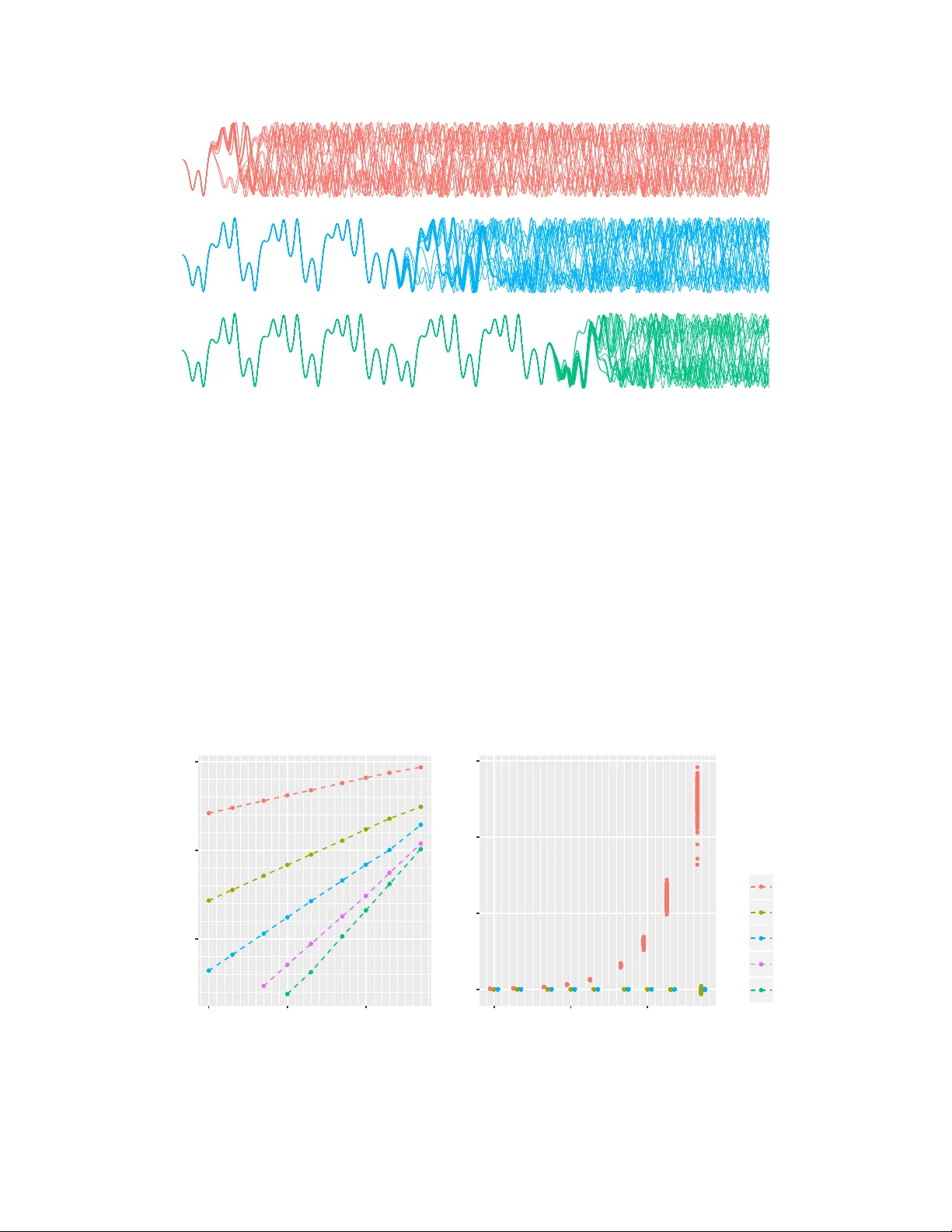
Pr obabilistic Linear Multistep Methods Onur T eymur Department of Mathematics Imperial College London o@teymur.uk Konstantinos Zygalakis School of Mathematics Univ ersity of Edinb urgh k.zygalakis@ed.ac.uk Ben Calderhead Department of Mathematics Imperial College London b.calderhead@imperial.ac.uk Abstract W e present a deriv ation and theoretical in v estigation of the Adams-Bashforth and Adams-Moulton family of linear multistep methods for solving ordinary dif ferential equations, starting from a Gaussian process (GP) frame work. In the limit, this formulation coincides with the classical deterministic methods, which ha ve been used as higher-order initial v alue problem solvers for ov er a century . Furthermore, the natural probabilistic frame work pro vided by the GP formulation allows us to deriv e pr obabilistic versions of these methods, in the spirit of a number of other probabilistic ODE solvers presented in the recent literature [1, 2, 3, 4] . In contrast to higher-order Runge-K utta methods, which require multiple intermediate function ev aluations per step, Adams f amily methods make use of previous function e v alua- tions, so that increased accuracy arising from a higher-order multistep approach comes at very little additional computational cost. W e show that through a careful choice of co v ariance function for the GP , the posterior mean and standard de viation ov er the numerical solution can be made to exactly coincide with the v alue given by the deterministic method and its local truncation error respecti vely . W e provide a rigorous proof of the con ver gence of these new methods, as well as an empirical in vestigation (up to fifth order) demonstrating their conv er gence rates in practice. 1 Introduction Numerical solvers for differential equations are essential tools in almost all disciplines of applied mathematics, due to the ubiquity of real-world phenomena described by such equations, and the lack of exact solutions to all b ut the most trivial examples. The performance – speed, accurac y , stability , robustness – of the numerical solver is of great relev ance to the practitioner . This is particularly the case if the computational cost of accurate solutions is significant, either because of high model complexity or because a high number of repeated ev aluations are required (which is typical if an ODE model is used as part of a statistical inference procedure, for example). A field of work has emerged which seeks to quantify this performance – or indeed lack of it – by modelling the numerical errors pr obabilistically , and thence trace the ef fect of the chosen numerical solver through the entire computational pipeline [5]. The aim is to be able to mak e meaningful quantitati ve statements about the uncertainty present in the resulting scientific or statistical conclusions. Recent work in this area has resulted in the development of probabilistic numerical methods, first conceiv ed in a very general w ay in [6]. An recent summary of the state of the field is giv en in [7]. The particular case of ODE solv ers was first addressed in [8], formalised and extended in [1, 2, 3] with a number of theoretical results recently gi ven in [4]. The present paper modifies and extends the constructions in [1, 4] to the multistep case, improving the order of con vergence of the method but av oiding the simplifying linearisation of the model required by the approaches of [2, 3]. Furthermore we offer extensions to the con vergence results in [4] to our proposed method and giv e empirical results confirming con ver gence rates which point to the practical usefulness of our higher-order approach without significantly increasing computational cost. 30th Conference on Neural Information Processing Systems (NIPS 2016), Barcelona, Spain. 1.1 Mathematical setup W e consider an Initial V alue Problem (IVP) defined by an ODE d d t y ( t, θ ) = f ( y ( t, θ ) , t ) , y ( t 0 , θ ) = y 0 (1) Here y ( · , θ ) : R + → R d is the solution function, f : R d × R + → R d is the vector -v alued function that defines the ODE, and y 0 ∈ R d is a giv en vector called the initial v alue. The dependence of y on an m -dimensional parameter θ ∈ R m will be relev ant if the aim is to incorporate the ODE into an in verse problem framework, and this parameter is of scientific interest. Bayesian inference under this setup (see [9]) is covered in most of the other treatments of this topic but is not the main focus of this paper; we therefore suppress θ for the sake of clarity . Some technical conditions are required in order to justify the existence and uniqueness of solutions to (1) . W e assume that f is ev aluable point-wise gi ven y and t and also that it satisfies the Lipschitz condition in y , namely || f ( y 1 , t ) − f ( y 2 , t ) || ≤ L f || y 1 − y 2 || for some L f ∈ R + and all t, y 1 and y 2 ; and also is continuous in t . These conditions imply the existence of a unique solution, by a classic result usually known as the Picard-Lindelöf Theorem [10]. W e consider a finite-dimensional discretisation of the problem, with our aim being to numerically generate an N -dimensional vector 1 y 1 : N approximating the true solution y ( t 1 : N ) in an appropriate sense. Following [1], we consider the joint distribution of y 1 : N and the auxiliary v ariables f 0 : N (obtained by ev aluating the function f ), with each y i obtained by sequentially conditioning on previous e valuations of f . A basic requirement is that the marginal mean of y 1 : N should correspond to some deterministic iterati ve numerical method operating on the grid t 1 : N . In our case this will be a linear multistep method (LMM) of specified type. 2 Firstly we telescopically factorise the joint distrib ution as follows: p ( y 1 : N , f 0 : N | y 0 ) = p ( f 0 | y 0 ) N − 1 Y i =0 p ( y i +1 | y 0 : i , f 0 : i ) p ( f i +1 | y 0 : i +1 , f 0 : i ) (2) W e can now make simplifying assumptions about the constituent distributions. Firstly since we hav e assumed that f is e v aluable point-wise gi ven y and t , p ( f i | y i , . . . ) = p ( f i | y i ) = δ f i  f ( y i , t i )  , (3) which is a Dirac-delta measure equivalent to simply performing this ev aluation deterministically . Secondly , we assume a finite moving window of dependence for each new state – in other words y i +1 is only allo wed to depend on y i and f i , f i − 1 , . . . , f i − ( s − 1) for some s ∈ N . This corresponds to the inputs used at each iteration of the s -step Adams-Bashforth method. For i < s we will assume dependence on only those deriv ative e valuations up to i ; this initialisation detail is discussed briefly in Section 4. Strictly speaking, f N is superfluous to our requirements (since we already hav e y N ) and thus we can rewrite (2) as p ( y 1 : N , f 0 : N − 1 | y 0 ) = N − 1 Y i =0 p ( f i | y i ) p ( y i +1 | y i , f max(0 ,i − s +1) : i ) (4) = N − 1 Y i =0 δ f i ( f ( y i , t i )) p ( y i +1 | y i , f max(0 ,i − s +1) : i ) | {z } ∗ (5) The conditional distributions ∗ are the primary objects of our study – we will define them by constructing a particular Gaussian process prior o ver all v ariables, then identifying the appropriate (Gaussian) conditional distribution. Note that a simple modification to the decomposition (2) allows the same set-up to generate an ( s + 1) -step Adams-Moulton iterator 3 – the implicit multistep method where y i +1 depends in addition on f i +1 . At various stages of this paper this extension is noted b ut omitted for reasons of space – the collected results are giv en in Appendix C. 1 The notation y 0 : N denotes the vector ( y 0 , . . . , y N ) , and analogously t 0 : N , f 0 : N etc. 2 W e argue that the connection to some specific deterministic method is a desirable feature, since it aids interpretability and allows much of the well-de veloped theory of IVP solvers to be inherited by the probabilistic solver . This is a particular strength of the formulation in [4] which was lacking in all previous works. 3 The con vention is that the number of steps is equal to the total number of deri vati ve e v aluations used in each iteration, hence the s -step AB and ( s + 1) -step AM methods both go ‘equally far back’. 2 Linear multistep methods W e giv e a very short summary of Adams family LMMs and their con ventional deri vation via interpolating polynomials. For a fuller treatment of this well-studied topic we refer the reader to the comprehensiv e references [10, 11, 12]. Using the usual notation we write y i for the numerical estimate of the true solution y ( t i ) , and f i for the estimate of f ( t i ) ≡ y 0 ( t i ) . The classic s -step Adams-Bashforth method calculates y i +1 by constructing the unique polynomial P i ( ω ) ∈ P s − 1 interpolating the points { f i − j } s − 1 j =0 . This is given by Lagrange’ s method as P i ( ω ) = s − 1 X j =0 ` 0 : s − 1 j ( ω ) f i − j ` 0 : s − 1 j ( ω ) = s − 1 Y k =0 k 6 = j ω − t i − k t i − j − t i − k (6) The ` 0 : s − 1 j ( ω ) are known as Lagrange polynomials, ha ve the property that ` 0 : s − 1 p ( t i − q ) = δ pq , and form a basis for the space P s − 1 known as the Lagrange basis. The Adams-Bashforth iteration then proceeds by writing the integral version of (1) as y ( t i +1 ) − y ( t i ) ≡ R t i +1 t i f ( y , t ) d t and approximating the function under the integral by the e xtrapolated interpolating polynomial to giv e y i +1 − y i ≈ Z t i +1 t i P i ( ω ) d ω = h s − 1 X j =0 β AB j,s f i − j (7) where h = t i +1 − t i and the β AB j,s ≡ h − 1 R h 0 ` 0 : s − 1 j ( ω ) d ω are the Adams-Bashforth coefficients for order s , all independent of h and summing to 1. Note that if f is a polynomial of de gree s − 1 (so y ( t ) is a polynomial of de gree s ) this procedure will gi ve the next solution v alue exactly . Otherwise the extrapolation error in f i +1 is of order O ( h s ) and in y i +1 (after an integration) is of order O ( h s +1 ) . So the local truncation error is O ( h s +1 ) and the global error O ( h s ) [10]. Adams-Moulton methods are similar except that the polynomial Q i ( ω ) ∈ P s interpolates the s + 1 points { f i − j } s − 1 j = − 1 . The resulting equation analogous to (7) is thus an implicit one, with the unknown y i +1 appearing on both sides. T ypically AM methods are used in conjunction with an AB method of one order lower , in a ‘predictor-corrector’ arrangement. Here, a predictor value y ∗ i +1 is calculated using an AB step; this is then used to estimate f ∗ i +1 = f ( y ∗ i +1 ) ; and finally an AM step uses this value to calculate y i +1 . W e again refer the reader to Appendix C for details of the AM construction. 2 Derivation of Adams family LMMs via Gaussian pr ocesses W e now consider a formulation of the Adams-Bashforth family starting from a Gaussian process framew ork and then present a probabilistic extension. W e fix a joint Gaussian process prior over y i +1 , y i , f i , f i − 1 , . . . , f i − s +1 as follo ws. W e define two vectors of functions φ ( ω ) and Φ( ω ) in terms of the Lagrange polynomials ` 0 : s − 1 j ( ω ) defined in (6) as φ ( ω ) =  0 ` 0 : s − 1 0 ( ω ) ` 0 : s − 1 1 ( ω ) . . . ` 0 : s − 1 s − 1 ( ω )  T (8) Φ( ω ) = Z φ ( ω ) d ω =  1 Z ` 0 : s − 1 0 ( ω ) d ω . . . Z ` 0 : s − 1 s − 1 ( ω ) d ω  T (9) The elements (excluding the first) of φ ( ω ) form a basis for P s − 1 and the elements of Φ( ω ) form a basis for P s . The initial 0 in φ ( ω ) is necessary to mak e the dimensions of the tw o v ectors equal, so we can correctly define products such as Φ( ω ) T φ ( ω ) which will be required later . The first element of Φ( ω ) can be an y non-zero constant C ; the analysis later is unchanged and we therefore tak e C = 1 . Since we will solely be interested in values of the ar gument ω corresponding to discrete equispaced time-steps t j − t j − 1 = h index ed relati ve to the current time-point t i = 0 , we will make our notation more concise by writing φ i + k for φ ( t i + k ) , and similarly Φ i + k for Φ( t i + k ) . W e no w use these v ectors of basis functions to define a joint Gaussian process prior as follows: 3           y i +1 y i f i f i − 1 . . . f i − s +1           = N                     0 0 0 0 . . . 0           ,           Φ T i +1 Φ i +1 Φ T i +1 Φ i Φ T i +1 φ i · · · Φ T i +1 φ i − s +1 Φ T i Φ i +1 Φ T i Φ i Φ T i φ i · · · Φ T i φ i − s +1 φ T i Φ i +1 φ T i Φ i φ T i φ i . . . φ T i φ i − s +1 φ T i − 1 Φ i +1 φ T i − 1 Φ i φ T i − 1 φ i . . . φ T i − 1 φ i − s +1 . . . . . . . . . . . . . . . φ T i − s +1 Φ i +1 φ T i − s +1 Φ i φ T i − s +1 φ i . . . φ T i − s +1 φ i − s +1                     (10) This construction works because y 0 = f and differentiation is a linear operator; the rules for the transformation of the co variance elem ents is gi ven in Section 9.4 of [13] and can easily be seen to correspond to the defined relationship between φ ( ω ) and Φ( ω ) . Recalling the decomposition in (5) , we are interested in the conditional distribution p ( y i +1 | y i , f i − s +1 : i ) . This is also Gaussian, with mean and cov ariance gi ven by the standard formulae for Gaussian conditioning. This construction now allo ws us to state the follo wing result: Proposition 1. The conditional distribution p ( y i +1 | y i , f i − s +1 : i ) under the Gaussian pr ocess prior given in (10) , with covariance k ernel basis functions as in (8) and (9) , is a δ -measur e concentrated on the s -step Adams-Bashforth pr edictor y i + h P s − 1 j =0 β AB j,s f i − j . The proof of this proposition is giv en in Appendix A. Because of the natural probabilistic structure pro vided by the Gaussian process frame work, we can augment the basis function vectors φ ( ω ) and Φ( ω ) to generate a conditional distribution for y i +1 that has non-zero variance. By choosing a particular form for this augmented basis we can obtain an expression for the standard deviation of y i +1 that is exactly equal to the leading-order local truncation error of the corresponding deterministic method. W e will expand the vectors φ ( ω ) and Φ( ω ) by one component, chosen so that the new v ector comprises elements that span a polynomial space of order one greater than before. Define the augmented bases φ + ( ω ) and Φ + ( ω ) as φ ( ω ) + =  0 ` 0 : s − 1 0 ( ω ) ` 0 : s − 1 1 ( ω ) . . . ` 0 : s − 1 s − 1 ( ω ) αh s ` − 1 : s − 1 − 1 ( ω )  T (11) Φ( ω ) + =  1 Z ` 0 : s − 1 0 ( ω ) d ω . . . Z ` 0 : s − 1 s − 1 ( ω ) d ω Z αh s ` − 1 : s − 1 − 1 ( ω ) d ω  T (12) The additional term at the end of φ + ( ω ) is the polynomial of order s which arises from interpolating f at s + 1 points (with the additional point at t i +1 ) and choosing the basis function corresponding to the root at t i +1 , scaled by αh s with α a positiv e constant whose role will be explained in the next section. The elements of these vectors span P s and P s +1 respectiv ely . With this ne w basis we can giv e the following result: Proposition 2. The conditional distribution p ( y i +1 | y i , f i − s +1 : i ) under the Gaussian pr ocess prior given in (10) , with covariance kernel basis functions as in (11) and (12) , is Gaussian with mean equal to the s -step Adams-Bashforth pr edictor y i + h P s − 1 j =0 β AB j,s f i − j and, setting α = y ( s +1) ( η ) for some η ∈ ( t i − s +1 , t i +1 ) , standar d deviation equal to its local truncation err or . The proof is giv en in Appendix B. In order to de-mystify the construction, we now exhibit a concrete example for the case s = 3 . The conditional distribution of interest is p ( y i +1 | y i , f i , f i − 1 , f i − 2 ) ≡ p ( y i +1 | y i , f i : i − 2 ) . In the deterministic case, the vectors of basis functions become φ ( ω ) s =3 =  0 ( ω + h )( ω + 2 h ) 2 h 2 ω ( ω + 2 h ) − h 2 ω ( ω + h ) 2 h 2  Φ( ω ) s =3 =  1 ω  2 ω 2 + 9 hω + h 2  12 h 2 ω 2 ( ω + 3 h ) − 3 h 2 ω 2 (2 ω + 3 h ) 12 h 2  4 and simple calculations giv e that E ( y i +1 | y i , f i : i − 2 ) = y i + h  23 12 f i − 4 3 f i − 1 + 5 12 f i − 2  V ar( y i +1 | y i , f i : i − 2 ) = 0 The probabilistic version follo ws by setting φ + ( ω ) s =3 =  0 ( ω + h )( ω + 2 h ) 2 h 2 ω ( ω + 2 h ) − h 2 ω ( ω + h ) 2 h 2 αω ( ω + h )( ω + 2 h ) 6  Φ + ( ω ) s =3 =  1 ω  2 ω 2 + 9 hω + h 2  12 h 2 ω 2 ( x + 3 h ) − 3 h 2 ω 2 (2 ω + 3 h ) 12 h 2 αω 2 ( ω + 2 h ) 2 24  and further calculation shows that E ( y i +1 | y i , f i : i − 2 ) = y i + h  23 12 f i − 4 3 f i − 1 + 5 12 f i − 2  V ar( y i +1 | y i , f i : i − 2 ) =  3 h 4 α 8  2 An entirely analogous argument can be sho wn to reproduce and probabilistically extend the implicit Adams-Moulton scheme. The Gaussian process prior now includes f i +1 as an additional variable and the correlation structure and v ectors of basis functions are modified accordingly . The required modifications are giv en in Appendix C and a explicit deriv ation for the 4-step AM method is given in Appendix D. 2.1 The role of α Replacing α in (11) by y ( s +1) ( η ) , with η ∈ ( t i − s +1 , t i +1 ) , makes the variance of the integrator coincide exactly with the local truncation error of the underlying deterministic method. 4 This is of course of limited utility unless higher derivati ves of y ( t ) are available, and ev en if they are, η is itself unkno wable in general. Howe ver it is possible to estimate the integrator v ariance in a systematic way by using backward dif ference approximations [14] to the required deriv ati ve at t i +1 . W e show this by e xpanding the s -step Adams-Bashforth iterator as y i +1 = y i + h P s − 1 j =0 β AB j,s f i − j + h s +1 C AB s y ( s +1) ( η ) η ∈ [ t i − s +1 , t i +1 ] = y i + h P s − 1 j =0 β AB j,s f i − j + h s +1 C AB s y ( s +1) ( t i +1 ) + O ( h s +2 ) = y i + h P s − 1 j =0 β AB j,s f i − j + h s +1 C AB s f ( s ) ( t i +1 ) + O ( h s +2 ) since y 0 = f = y i + h P s − 1 j =0 β AB j,s f i − j + h s +1 C AB s h h − s P s − 1+ p k =0 δ k,s − 1+ p f i − k + O ( h p ) i + O ( h s +2 ) = y i + h P s − 1 j =0 β AB j,s f i − j + hC AB s P s k =0 δ k,s f i − k + O ( h s +2 ) if we set p = 1 (13) where β AB · ,s are the set of coefficients and C AB s the local truncation error constant for the s -step Adams-Bashforth method, and δ · ,s − 1+ p are the set of backward difference coef ficients for estimating the s th deriv ativ e of f to order O ( h p ) [14]. In other words, the constant α can be substituted with h − s P s k =0 δ k,s f i − k , using already a vailable function values and to adequate order . It is worth noting that collecting the coefficients β AB · ,s and δ · ,s results in an expression equi valent to the Adams-Bashforth method of order s + 1 and therefore, this procedure is in ef fect emplo ying two integrators of dif ferent orders and estimating the truncation error from the dif ference of the tw o. 5 This principle is similar to the classical Milne De vice [12], which pairs an AB and and AM iterator to achie ve the same thing. Using the Milne Device to generate a v alue for the error variance is also straightforward within our frame work, but requires two e valuations of f at each iteration (one of which immediately goes to waste) instead of the approach presented here, which only requires one. 4 W e do not claim that this is the only possible way of modelling the numerical error in the solver . The question of how to do this accurately is an open problem in general, and is particularly challenging in the multi-dimensional case. In many real world problems different noise scales will be appropriate for different dimensions and – especially in ‘hierarchical’ models arising from higher-order ODEs – non-Gaussian noise is to be expected. That said, the Gaussian assumption as a first order approximation for numerical error is present in virtually all work on this subject and goes all the way back to [8]. W e adopt this premise throughout, whilst noting this interesting unresolved issue. 5 An explicit deri v ation of this for s = 3 is giv en in Appendix E. 5 3 Con vergence of the pr obabilistic Adams-Bashf orth integrator W e now gi ve the main result of our paper , which demonstrates that the conv er gence properties of the probabilistic Adams-Bashforth integrator match those of its deterministic counterpart. Theorem 3. Consider the s -step deterministic Adams-Bashforth inte grator given in Pr oposition 1, which is of or der s . Then the pr obabilistic inte grator constructed in Pr oposition 2 has the same mean squar e err or as its deterministic counterpart. In particular max 0 ≤ kh ≤ T E | Y k − y k | 2 ≤ K h 2 s wher e Y k ≡ y ( t k ) denotes the true solution, y k the numerical solution, and K is a positive real number depending on T but independent of h . The proof of this theorem is gi ven in Appendix F, and follo ws a similar line of reasoning to that gi ven for a one-step probabilistic Euler inte grator in [4]. In particular , we deduce the con vergence of the algorithm by extrapolating from the local error . The additional complexity arises due to the presence of the stochastic part, which means we cannot rely directly on the theory of dif ference equations and the representations of their solutions. Instead, following [15], we rewrite the defining s -step recurrence equation as a one-step recurrence equation in a higher dimensional space. 4 Implementation W e now hav e an implementable algorithm for an s -step probabilistic Adams-Bashforth integrator . Firstly , an accurate initialisation is required for the first s iterations – this can be achie ved with, for example, a Runge-K utta method of suf ficiently high order . 6 Secondly , at iteration i , the preceding s stored function e valuations are used to find the posterior mean and v ariance of y i +1 . The integrator then adv ances by generating a realisation of the posterior measure deriv ed in Proposition 2. Following [1], a Monte Carlo repetition of this procedure with dif ferent random seeds can then be used as an effecti ve way of generating propagated uncertainty estimates at an y time 0 < T < ∞ . 4.1 Example – Chua circuit The Chua circuit [16] is the simplest electronic circuit that exhibits chaotic beha viour, and has been the subject of extensi ve study – in both the mathematics and electronics communities – for ov er 30 years. Readers interested in this rich topic are directed to [17] and the references therein. The defining characteristic of chaotic systems is their unpredictable long-term sensitivity to tiny changes in initial conditions, which also manifests itself in the sudden amplification of error introduced by any numerical scheme. It is therefore of interest to understand the limitations of a gi ven numerical method applied to such a problem – namely the point at which the solution can no longer be taken to be a meaningful approximation of the ground truth. Probabilistic integrators allow us to do this in a natural way [1]. The Chua system is giv en by x 0 = α ( y − (1 + h 1 ) x − h 3 x 3 ) , y 0 = x − y + z , z 0 = − β y − γ z . W e use parameter values α = − 1 . 4157 , β = 0 . 02944201 , γ = 0 . 322673579 , h 1 = − 0 . 0197557699 , h 3 = − 0 . 0609273571 and initial conditions x 0 = 0 , y 0 = 0 . 003 , z 0 = 0 . 005 . This particular choice is taken from ‘ Attractor CE96’ in [18]. Using the probabilistic version of the Adams-Bashforth integrator with s > 1 , it is possible to delay the point at which numerical path div erges from the truth, with effectively no additional evaluations of f r equir ed compared to the one-step method. This is demonstrated in Figure 1. Our approach is therefore able to combine the benefits of classical higher-order methods with the additional insight into solution uncertainty provided by a probabilistic method. 4.2 Example – Lotka-V olterra model W e now apply the probabilistic integrator to a simple periodic predator-pre y model given by the system x 0 = αx − β xy , y 0 = γ xy − δ y for parameters α = 1 , β = 0 . 3 , γ = 1 and δ = 0 . 7 . W e demonstrate the con vergence beha viour stated in Theorem 3 empirically . 6 W e use a (packaged) adaptive Runge-K utta-Fehlberg solv er of 7th order with 8th order error control. 6 Figure 1: Time series for the x -component in the Chua circuit model described in Section 4.1, solved 20 times for 0 ≤ t ≤ 1000 using an s -step probabilistic AB inte grator with s = 1 (top), s = 3 (middle), s = 5 (bottom). Step-size remains h = 0 . 01 throughout. W all-clock time for each simulation was close to constant ( ± 10 per cent – the dif ference primarily accounted for by the RKF initialisation procedure). The left-hand plot in Figure 2 shows the sample mean of the absolute error of 200 realisations of the probabilistic integrator plotted ag ainst step-size, on a log-log scale. The differing orders of con vergence of the probabilistic integrators are easily deduced from the slopes of the lines sho wn. The right-hand plot sho ws the actual error v alue (no logarithm or absolute v alue taken) of the same 200 realisations, plotted individually against step-size. This plot shows that the error in the one-step integrator is consistently positi ve, whereas for two- and three-step integrators is approximately centred around 0. (This is also visible with the same data if the plot is zoomed to more closely examine the range with small h .) Though this phenomenon can be expected to be somewhat problem-dependent, it is certainly an interesting observ ation which may ha ve implications for bias reduction in a Bayesian in verse problem setting. −10 −5 0 −4 −3 −2 log10 h log10 E |Error| 0.0 0.2 0.4 0.6 −4 −3 −2 log10 h Error No . of steps (s) 1 2 3 4 5 Figure 2: Empirical error analysis for the x -component of 200 realisations of the probabilistic AB integrator as applied to the Lotka-V olterra model described in Section 4.2. The left-hand plot shows the con ver gence rates for AB integrators of orders 1-5, while the right-hand plot shows the distrib ution of error around zero for integrators of orders 1-3. 7 5 Conclusion W e have gi ven a deriv ation of the Adams-Bashforth and Adams-Moulton families of linear multistep ODE integrators, making use of a Gaussian process framework, which we then extend to develop their probabilistic counterparts. W e have sho wn that the deriv ed family of probabilistic integrators result in a posterior mean at each step that exactly coincides with the corresponding deterministic inte grator , with the posterior standard deviation equal to the deterministic method’ s local truncation error . W e hav e giv en the general forms of the construction of these ne w integrators to arbitrary order . Furthermore, we hav e inv estigated their theoretical properties and pro vided a rigorous proof of their rates of con ver gence, Finally we hav e demonstrated the use and computational efficienc y of probabilistic Adams-Bashforth methods by implementing the solvers up to fifth order and providing e xample solutions of a chaotic system, and well as empirically verifying the con vergence rates in a Lotka-V oltera model. W e hope the ideas presented here will add to the arsenal of any practitioner who uses numerical methods in their scientific analyses, and contributes a further tool in the emer ging field of probabilistic numerical methods. References [1] O . A . C H K R E B T I I , D . A . C A M P B E L L , B . C A L D E R H E A D , and M . A . G I R O L A M I . Bayesian Solution Uncertainty Quantification for Differential Equations. Bayesian Analysis , 2016. [2] P . H E N N I G and S . H AU B E R G . Probabilistic Solutions to Differential Equations and their Application to Riemannian Statistics. In, Pr oc. of the 17th int. Conf. on Artificial Intelligence and Statistics (AIST A TS) . V olume 33. JMLR, W&CP, 2014. [3] M . S C H O B E R , D . K . D U V E NAU D , and P . H E N N I G . Probabilistic ODE Solvers with Runge-Kutta Means. In Z . G H A H R A M A N I , M . W E L L I N G , C . C O RT E S , N . D . L AW R E N C E , and K . Q . W E I N B E R G E R , editors, Advances in Neural Information Pr ocessing Systems 27 , pages 739–747. Curran Associates, Inc., 2014. [4] P . R . C O N R A D , M . G I RO L A M I , S . S Ä R K K Ä , A . S T UA RT , and K . Z Y G A L A K I S . Statistical Analysis of Differential Equations: Introducing Probability Measures on Numerical Solutions. Statistics and Computing , 2016. [5] M . C . K E N N E DY and A . O ’ H A G A N . Bayesian Calibration of Computer Models. J ournal of the Royal Statistical Society: Series B , 63(3):425–464, 2001. [6] P . D I AC O N I S . Bayesian Numerical Analysis. In J . B E R G E R and S . G U P TA , editors, Statistical Decision Theory and Related T opics IV . V olume 1, pages 163–175. Springer, 1988. [7] P . H E N N I G , M . A . O S B O R N E , and M . G I RO L A M I . Probabilistic Numerics and Uncertainty in Computa- tions. Pr oc. R. Soc. A , 471(2179):20150142, 2015. [8] J . S K I L L I N G . Bayesian Numerical Analysis. In J . W. T . G R A N DY and P . W . M I L O N N I , editors, Physics and Pr obability , pages 207–222. Cambridge University Press, 1993. [9] M . G I R O L A M I . Bayesian Inference for Differential Equations. Theor . Comp. Sci. , 408(1):4–16, 2008. [10] A . I S E R L E S . A Fir st Course in the Numerical Analysis of Differ ential Equations . Cambridge Uni versity Press, 2nd edition, 2008. [11] E . H A I R E R , S . N Ø R S E T T , and G . W A N N E R . Solving Or dinary Diff er ential Equations I: Nonstiff Pr oblems . Springer Series in Computational Mathematics. Springer, 2008. [12] J . B U T C H E R . Numerical Methods for Or dinary Differ ential Equations: Second Edition . W iley, 2008. [13] C . R A S M U S S E N and C . W I L L I A M S . Gaussian Pr ocesses for Machine Learning . Univ ersity Press Group Limited, 2006. [14] B . F O R N B E R G . Generation of Finite Difference Formulas on Arbitrarily Spaced Grids. Mathematics of Computation , 51(184):699–706, 1988. [15] E . B U C K W A R and R . W I N K L E R . Multistep Methods for SDEs and Their Application to Problems with Small Noise. SIAM J. Numer . Anal. , 44(2):779–803, 2006. [16] L . O . C H U A . The Genesis of Chua’ s Circuit. Arc hiv für Elektr onik und Übertragungstec hnik , 46(4):250– 257, 1992. [17] L . O . C H UA . Chua Circuit. Scholarpedia , 2(10):1488, 2007. [18] E . B I L OT TA and P . P AN T A N O . A Gallery of Chua Attractors . W orld Scientific, 2008. KZ was partially supported by a grant from the Simons F oundation. Part of this work was done during the author’ s stay at the Newton Institute for the programme Stoc hastic Dynamical Systems in Biology: Numerical Methods and Applications. 8 A ppendices A Proof of Pr oposition 1 Recall that h = t j − t j − 1 for all j . Straightforward substitutions into the definitions gi ve that φ i ≡ φ (0) = (0 , 1 , 0 , . . . , 0) , φ i − 1 ≡ φ ( − h ) = (0 , 0 , 1 , . . . , 0) etc. and hence φ T i − p φ i − q = δ pq , for all 0 ≤ p, q ≤ s − 1 . Furthermore Φ i ≡ Φ(0) = (1 , 0 , 0 , . . . , 0) since ev ery component of Φ( ω ) bar the first is a polynomial of degree s with a factor ω . Finally Φ i +1 ≡ Φ( h ) =  1 Z h 0 ` 0 : s − 1 0 ( ω ) d ω . . . Z h 0 ` 0 : s − 1 s − 1 ( ω ) d ω  Now by (10) and the standard formulae for Gaussian conditioning, we ha ve E [ y i +1 | y i ,f i − s +1 : i ] =      Φ T i +1 Φ i Φ T i +1 φ i . . . Φ T i +1 φ i − s +1      T      Φ T i Φ i Φ T i φ i · · · Φ T i φ i − s +1 φ T i Φ i φ T i φ i · · · φ T i φ i − s +1 . . . . . . . . . . . . φ T i − s +1 Φ i φ T i − s +1 φ i +1 . . . φ T i − s +1 φ i − s +1      − 1 | {z } I − 1 s +1      y i f i . . . f i − s +1      = (Φ T i +1 Φ i ) y i + s − 1 X k =0 (Φ T i +1 φ i − k ) f i − k = y i + s − 1 X k =0 [Φ i +1 ] k +2 · f i − k  where [Φ i +1 ] k +2 denotes the ( k + 2) th component of Φ i +1  = y i + s − 1 X k =0 " Z h 0 ` 0 : s − 1 k ( ω ) d ω # · f i − k = y i + h s − 1 X k =0 c k,s f i − k since Z h 0 ` 0 : s − 1 k ( ω ) d ω = hc k,s which is equal to the s -step Adams-Bashforth predictor defined by (6) and (7). Next we write V ar[ y i +1 | y i , f i − s +1 : i ] = Φ T i +1 Φ i +1 −      Φ T i +1 Φ i Φ T i +1 φ i . . . Φ T i +1 φ i − s +1      T I − 1 s +1      Φ T i Φ i +1 φ T i Φ i +1 . . . φ T i − s +1 Φ i +1      = Φ T i +1 Φ i +1 −      1 [Φ i +1 ] 2 . . . [Φ i +1 ] s +1      T      1 [Φ i +1 ] 2 . . . [Φ i +1 ] s +1      = Φ T i +1 Φ i +1 − Φ T i +1 Φ i +1 = 0 and the proposition follows. B Proof of Pr oposition 2 W e follow the same reasoning as in Proposition 1. Since the additional basis function at the end of φ + i − k is clearly zero at for all 0 ≤ k ≤ s − 1 , each inner product of the form φ + T φ + , Φ + T φ + and φ + T Φ + is equal to the corresponding inner product φ T φ , Φ T φ and φ T Φ as no additional i contribution from the ne w extended basis arises. It therefore suffices to check only the terms of the form Φ + T Φ . Integrating the additional basis function gi ves a polynomial of de gree s + 1 with a constant factor ω . Ev aluating this at t i = 0 means that the additional term is also 0 in Φ i . Therefore Φ + T i +1 Φ + i = Φ T i +1 Φ i and Φ + T i Φ + i = Φ T i Φ i . It follows that the expression for E [ y i +1 | y i , f i − s +1 : i ] is exactly the same as when using the unaugmented basis function set. The argument in the pre vious paragraph means we can immediately write down that V ar[ y i +1 | y i , f i − s +1 : i ] = Φ + T i +1 Φ + i +1 − Φ T i +1 Φ i +1 Since the first s + 1 components of Φ + T i +1 are equal to the s + 1 components of Φ T i +1 , this expression reduces to the contribution of the augmented basis element. Therefore V ar[ y i +1 | y i , f i − s +1 : i ] = αh s Z h 0 ` − 1 : s − 1 − 1 ( ω ) d ω ! 2 =  αh s +1 β AM − 1 ,s +1  2 The Adams-Moulton coefficient β AM − 1 ,s +1 is equal to the local truncation error constant for the s -step Adams-Bashforth method [12] and the proposition follows. C Extension to Adams-Moulton W e collect here the straightforward modifications required to the constructions in the main paper to produce implicit Adams-Moulton methods instead of explicit Adams-Bashforth v ersions. The telescopic decomposition (5) becomes p ( y 1 : N , f 0 : N | y 0 ) = N Y i =0 p ( f i | y i ) × N − 1 Y i =0 p ( y i +1 | y i , f max(0 ,i − s +1) : i +1 ) (14) where it is particularly to be noted that f N is no longer superfluous. The Lagrange interpolation resulting in the the Adams-Moulton method is Q i ( ω ) = s − 1 X j = − 1 ` − 1 : s − 1 j ( ω ) f i − j ` − 1 : s − 1 j ( ω ) = s − 1 Y k = − 1 k 6 = j ω − t i − k t i − j − t i − k , (15) the analogous vectors of basis polynomials to (8) and (9) are ψ ( ω ) =  0 ` − 1 : s − 1 − 1 ( ω ) ` − 1 : s − 1 0 ( ω ) ` − 1 : s − 1 1 ( ω ) . . . ` − 1 : s − 1 s − 1 ( ω )  T (16) Ψ( ω ) = Z ψ ( ω ) d ω =  1 Z ` − 1 : s − 1 − 1 ( ω ) d ω . . . Z ` − 1 : s − 1 s − 1 ( ω ) d ω  T (17) and the iterator is defined by y i +1 − y i ≈ Z t i +1 t i Q i ( ω ) d ω = h s − 1 X j = − 1 β AM j,s +1 f i − j (18) with β AM j,s +1 ≡ h − 1 Z h 0 ` − 1 : s − 1 j ( ω ) d ω are the Adams-Moulton coefficients. The Gaussian process prior resulting in AM is ii             y i +1 y i f i +1 f i f i − 1 . . . f i − s +1             = N                         0 0 0 0 0 . . . 0             ,             Ψ T i +1 Ψ i +1 Ψ T i +1 Ψ i Ψ T i +1 ψ i +1 · · · Ψ T i +1 ψ i − s +1 Ψ T i Ψ i +1 Ψ T i Ψ i Ψ T i ψ i +1 · · · Ψ T i ψ i − s +1 ψ T i +1 Ψ i +1 ψ T i +1 Ψ i ψ T i +1 ψ i +1 · · · ψ T i +1 ψ i − s +1 ψ T i Ψ i +1 ψ T i Ψ i ψ T i ψ i +1 · · · ψ T i ψ i − s +1 ψ T i − 1 Ψ i +1 ψ T i − 1 Ψ i ψ T i − 1 ψ i +1 · · · ψ T i − 1 ψ i − s +1 . . . . . . . . . . . . . . . ψ T i − s +1 Ψ i +1 ψ T i − s +1 Ψ i ψ T i − s +1 ψ i +1 · · · ψ T i − s +1 ψ i − s +1                         (19) D Adams-Moulton integrator with s = 4 The conditional distribution of interest is p ( y i +1 | y i , f i +1 , f i , f i − 1 , f i − 2 ) ≡ p ( y i +1 | y i , f i +1 : i − 2 ) . In the deterministic case the vectors of basis functions become ψ ( ω ) s =4 =  0 ω ( ω + h )( ω +2 h ) − 6 h 3 ( ω − h )( ω + h )( ω +2 h ) 2 h 3 ω ( ω − h )( ω +2 h ) − 2 h 3 ω ( ω − h )( ω + h ) 6 h 3  (20) Ψ( ω ) s =4 =  1 ω 2 (2 h + ω ) 2 24 h 3 ω (3 ω 3 +8 hω 2 − 6 h 2 ω − 2 f h 3 ) − 24 h 3 ω 2 (3 ω 2 +4 hω − 12 h 2 ) 24 h 3 ω 2 ( ω 2 − 2 h 2 ) − 24 h 3  (21) and the resulting calculations giv e E ( y i +1 | y i , f i +1 : i − 2 ) = y i + h  3 8 f i +1 + 19 24 f i − 5 24 f i − 1 + 1 24 f i − 2  V ar( y i +1 | y i , f i +1 : i − 2 ) = 0 The probabilistic version is ψ + ( ω ) s =4 =  · · · ψ ( ω ) s =4 · · · αω ( ω − h )( ω + h )( ω +2 h ) 24  (22) Ψ + ( ω ) s =4 =  · · · Ψ( ω ) s =4 · · · αω 2 (6 ω 3 +15 ω 2 h − 10 ωh 2 − 30 h 3 ) 720  (23) and further calculation shows that E ( y i +1 | y i , f i − 1 : i +2 ) = y i + h  3 8 f i +1 + 19 24 f i − 5 24 f i − 1 + 1 24 f i − 2  (24) V ar[ y i +1 | y i , f i +1 : i − 2 ] =  19 h 5 α 720  2 (25) Remark Proofs analogous to those of Propositions 1 and 2, for the Adams-Moulton case, follow the same line of reasoning as for the Adams-Bashforth case. E Expansion of backward difference coefficient appr oximation f or s = 3 From (13), we hav e for s = 3 y i +1 = y i + h  23 12 f i − 4 3 f i − 1 + 5 12 f i − 2  − 3 8 h 4 y (4) ( t i +1 ) + O ( h 5 ) = y i + h  23 12 f i − 4 3 f i − 1 + 5 12 f i − 2  − 3 8 h 4 f 000 ( t i +1 ) + O ( h 5 ) = y i + h  23 12 f i − 4 3 f i − 1 + 5 12 f i − 2  − 3 8 h 4  − f i + 3 f i − 1 − 3 f i − 2 + f i − 3 h 3 + O ( h )  + O ( h 5 ) = y i + h  55 24 f i − 59 24 f i − 1 + 37 24 f i − 2 − 3 8 f i − 3  | {z } AB4 + O ( h 5 ) iii F Proof of Theor em 3 Proposition 2 implies that our integrator can be written as y i +1 = y i + h s − 1 X j =0 β AB j,s f ( y i − j , t i − j ) + ξ i (26) where y i denotes the numerical solution at iteration i , and ξ i ∈ R d is a Gaussian random variable satisfying E | ξ i ξ T i | = Qh 2 s +2 for some fix ed d × d matrix Q . W e denote the true solution of the ODE (1) at iteration i by Y i ≡ y ( t i ) and we have that Y i +1 = Y i + h s − 1 X j =0 β AB j,s f ( Y i − j , t i − j ) + τ i (27) where by construction the local truncation error τ i = O ( h s +1 ) . If we no w subtract (26) from (27) and denote the accumulated error at iteration i by E i = Y i − y i , we hav e E i +1 = E i + ∆ φ i + τ i − ξ i where ∆ φ i : = h s − 1 X j =0 β AB j,s ∆ f i − j , ∆ f i − j : = f ( Y i − j , t i − j ) − f ( y i − j , t i − j ) W e will rearrange this s -step recursion to gi ve an equi valent one-step recursion in an higher - dimensional space. In particular , using the trivial identities E i − 1 = E i − 1 , · · · , E i − s +1 = E i − s +1 we obtain      E i +1 E i . . . E i − s +2      | {z } = : E i +1 =      I d 0 · · · 0 I d 0 · · · 0 . . . . . . 0 I d 0      | {z } = : A      E i E i − 1 . . . E i − s +1      | {z } = : E i +      ∆ φ i 0 . . . 0      | {z } = : ∆Φ i +      τ i 0 . . . 0      | {z } = : T i −      ξ i 0 . . . 0      | {z } = : Ξ i or in compact form, E i +1 = AE i + ∆Φ i + T i − Ξ i , i = s − 1 , . . . , N − 1 , N = T /h (28) For the subsequent calculations it will be necessary to find a scalar product inducing a matrix norm such that the norm of the matrix A is less or equal to 1 . This is possible if the eigen values of the Frobenius matrix A lie inside the unit circle on the complex plane and are simple if their modulus is equal to 1 . It is easy to sho w that the eigen values of A are roots of the characteristic polynomial associated with the deterministic integrator (7) . Since we hav e assumed that the deterministic integrator is con vergent, A does hav e the claimed property , since it is equiv alent to the root condition in Dahlquist’ s equiv alence theorem [12]. Thus there exists a non-singular matrix Λ with a block structure like A such that || Λ − 1 A Λ || 2 ≤ 1 . W e can therefore choose a scalar product for X , Y ∈ R ds as hX , Y i ∗ : =  Λ − 1 X , Λ − 1 Y  2 and then hav e | · | ∗ and || · || ∗ as the induced vector and matrix norms respectiv ely , with ||A|| ∗ = || Λ − 1 A Λ || 2 ≤ 1 as required. W e also have hX , Y i ∗ = X T Λ − T Λ − 1 Y = X T Λ ∗ Y with Λ ∗ = Λ − T Λ − 1 = ( λ ∗ ij ⊗ I d ) 1 ≤ i,j ≤ s (29) Due to the equiv alence of norms there exist constants c ∗ , c ∗ > 0 such that |X | 2 2 ≤ c ∗ |X | 2 ∗ and |X | 2 ∗ ≤ c ∗ |X | 2 ∞ for all X ∈ R ds , (30) where |X | 2 2 = P j =1 ,...,s | x j | 2 and |X | ∞ = max j =1 ,...,s | x j | for X = ( x T 1 , · · · , x T s ) T , x j ∈ R d . For the particular vectors ˜ X = ( x T , 0 , · · · , 0) T and ˜ Y = ( y T , 0 , · · · , 0) T with ˜ X , ˜ Y ∈ R ds and x, y ∈ R d , one has h ˜ X , ˜ Y i ∗ = λ ∗ 11 h x, y i 2 = λ ∗ 11 x T y , (31) iv where λ ∗ 11 is as in (29). Applying the norm | · | 2 ∗ to (28) and taking expectations gi ves E |E i +1 | 2 ∗ = E |AE i + ∆Φ i + T i − Ξ i | 2 ∗ = E |AE i + ∆Φ i + T i | 2 ∗ + O ( h 2 s +2 ) = E |AE i + ∆Φ i | 2 ∗ + 2 E h h 1 / 2 ( AE i + ∆Φ i ) , T i h − 1 / 2 i ∗ + E |T i | 2 ∗ + O ( h 2 s +2 ) = E |AE i + ∆Φ i | 2 ∗ + 2 E h h 1 / 2 ( AE i + ∆Φ i ) , T i h − 1 / 2 i ∗ + O ( h 2 s +2 ) (32) W e now consider the term |AE i + ∆Φ i | 2 ∗ and expand it as |AE i + ∆Φ i | 2 ∗ = |AE i | 2 ∗ | {z } A + | ∆Φ i | 2 ∗ | {z } B + 2 hAE i , ∆Φ i i ∗ | {z } C For term A we immediately ha ve |AE i | 2 ∗ ≤ |E i | 2 ∗ by construction of the norm | · | 2 ∗ . For term B we ha ve that | ∆Φ i | 2 ∗ = λ ∗ 11 | ∆ φ i | 2 from (31) = λ ∗ 11   h P s − 1 j =0 β AB j,s ∆ f i − j   2 ≤ λ ∗ 11 sh 2 P s − 1 j =0   β AB j,s ∆ f i − j   2 by Cauchy-Schwarz ≤ λ ∗ 11 sh 2 L 2 f P s − 1 j =0 ( β AB j,s ) 2 | E i − j | 2 since f is Lipschitz ≤ λ ∗ 11 sh 2 L 2 f C 2 β P s − 1 j =0 | E i − j | 2 where C 2 β = max j =0 ,...,s − 1 β AB j,s ≤ λ ∗ 11 sh 2 L 2 f C 2 β c ∗ |E i | 2 ∗ from (30) = : Γ 2 h 2 |E i | 2 ∗ where Γ 2 = λ ∗ 11 sL 2 f C 2 β c ∗ For term C we ha ve 2 hAE i , ∆Φ i i ∗ ≤ 2 |AE i | ∗ | ∆Φ i | ∗ ≤ 2Γ h |E i | 2 ∗ and it follows that |AE i + ∆Φ i | 2 ∗ ≤ (1 + O ( h )) |E i | 2 ∗ Then from (32) we hav e E |E i +1 | 2 ∗ = E |AE i + ∆Φ i | 2 ∗ + 2 E h h 1 / 2 ( AE i + ∆Φ i ) , T i h − 1 / 2 i ∗ + O ( h 2 s +2 ) ≤ (1 + O ( h )) E |E i | 2 ∗ + 2 h E |AE i + ∆Φ i | 2 ∗ + 2 h − 1 E |T i | 2 ∗ + O ( h 2 s +2 ) ≤ (1 + O ( h )) E |E i | 2 ∗ + O ( h 2 s +1 ) + O ( h 2 s +2 ) (33) Then by applying the Gronwall inequality we ha ve (for dif ferent K in each line) max 0 ≤ kh ≤ T E |E k | 2 ∗ ≤ K ( T ) h 2 s and since E k = ( E k , E k − 1 , · · · , E k − s +1 ) we conclude that max 0 ≤ kh ≤ T E | E k | 2 ≤ K ( T ) h 2 s Note that in (33) , the O ( h 2 s +2 ) term deriv ed from the introduced perturbations ξ i is of one higher order than the O ( h 2 s +1 ) term representing the truncation error in the deterministic solver . This observation implies that a noise vector satisfying E | ξ i ξ T i | = Qh 2 s +1 would also give rise to an integrator of order s . Remark An analogous proof for the Adams-Moulton case follows with straightforw ard modifications. v