Algorithmic Polarization for Hidden Markov Models

Using a mild variant of polar codes we design linear compression schemes compressing Hidden Markov sources (where the source is a Markov chain, but whose state is not necessarily observable from its output), and to decode from Hidden Markov channels (where the channel has a state and the error introduced depends on the state). We give the first polynomial time algorithms that manage to compress and decompress (or encode and decode) at input lengths that are polynomial $\it{both}$ in the gap to capacity and the mixing time of the Markov chain. Prior work achieved capacity only asymptotically in the limit of large lengths, and polynomial bounds were not available with respect to either the gap to capacity or mixing time. Our results operate in the setting where the source (or the channel) is $\it{known}$. If the source is $\it{unknown}$ then compression at such short lengths would lead to effective algorithms for learning parity with noise – thus our results are the first to suggest a separation between the complexity of the problem when the source is known versus when it is unknown.

💡 Research Summary

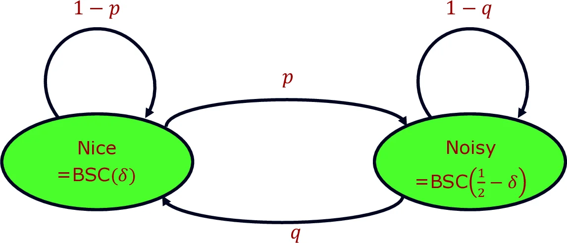
The paper tackles two closely related problems: lossless linear compression of hidden Markov sources and reliable communication over additive Markov channels. A hidden Markov source emits symbols from a finite alphabet according to a Markov chain whose states are not directly observable; an additive Markov channel adds a noise sequence generated by such a source to the transmitted codeword. The authors aim to achieve rates arbitrarily close to the Shannon capacity while keeping block length polynomial in both the gap to capacity ε and the mixing time τ of the underlying Markov chain.

The core technical contribution is a modest modification of Arıkan’s polar coding scheme. Instead of applying the classic 2×2 polar transform recursively, the authors select a prime‑field mixing matrix M∈F_q^{k×k} (invertible and non‑lower‑triangular under any column permutation) and apply M independently to each of t = n/k² blocks of size k. This “block‑wise polar transform” preserves the essential polarization properties proved by Blasiok et al. for mixing matrices, guaranteeing that a constant fraction of transformed bits become “good” (high entropy) and the rest “bad” (low entropy) at a rate that converges to the source entropy H(Z). Crucially, the analysis shows that the convergence is polynomially fast in 1/ε, and the block length needed is only poly(τ/ε). The mixing time appears because the source’s dependence decays exponentially; by grouping symbols into blocks larger than τ, the dependence across blocks becomes negligible, allowing the polar analysis to proceed as if the blocks were independent.

The algorithm consists of three stages:

1. Preprocessing (Polar‑Preprocess) – Given the Markov source description (transition matrix Π, emission distributions {S_i}) and a target block count t, the algorithm computes the conditional entropies of each transformed bit using the forward–backward algorithm for hidden Markov models. It identifies the set of good bits whose conditional entropy exceeds 1−ε and records the necessary side information S. This step runs in time poly(n,ℓ,1/ε), where ℓ is the number of hidden states.

2. Compression (Polar‑Compress) – The source output Z∈F_q^n is multiplied by the block‑wise matrix M^{⊗t}. Only the good bits (as indicated by S) are retained, yielding a compressed string \tilde U of length ≈ n·H(Z)+εn. The linear map can be implemented in O(n log n) time using fast matrix‑vector multiplication.

3. Decompression (Polar‑Decompress) – Using S, the decoder reconstructs the good bits, then applies the inverse transform (M^{-1})^{⊗t}. To recover the missing bad bits, the decoder runs a forward–backward inference on the hidden Markov model conditioned on the already recovered bits. The overall runtime is O(n^{3/2}·ℓ² + n log n). With probability at least 1−exp(−Ω(n)), the reconstruction error probability is O(1/n²).

Theorem 2.9 formalizes these guarantees for source compression. Theorem 2.10 translates them into a coding scheme for additive Markov channels: given a message of length r ≥ n·(1−H(Z)−ε), the encoder first compresses a random noise sequence Z drawn from the source, then adds the message to the compressed representation, and finally transmits the resulting codeword. The decoder, after receiving the noisy output, runs the same Polar‑Decompress routine to recover Z and consequently the original message. The achieved rate is within ε of the channel capacity C = 1−H(Z), and decoding error probability again decays as O(1/n²) with block length n > poly(τ/ε).

An important conceptual contribution is the separation between the “known‑source” and “unknown‑source” settings. The authors prove (Appendix B) that if one could compress an unknown hidden Markov source at block lengths polynomial in τ and 1/ε, one would obtain a polynomial‑time algorithm for learning parity with noise (LPN), a problem widely believed to be computationally hard. Hence, the existence of efficient compression in the known‑source case does not contradict existing hardness assumptions, but rather highlights a genuine complexity gap.

The paper also discusses practical considerations: the decoding complexity can be reduced to O(n^{1+δ}·ℓ² + n log n) by adjusting block dimensions, and the authors conjecture that with additional bookkeeping the runtime could be brought down to near‑linear O(n log n). Moreover, while the results are presented for additive channels over prime fields, the techniques extend to more general symmetric channels, though this extension is left for future work.

In summary, the authors deliver the first polynomial‑time, finite‑block‑length coding and compression constructions for hidden Markov models that are provably close to capacity. Their approach leverages modern polar‑code analysis, mixing‑matrix theory, and hidden‑Markov inference to bridge the gap between asymptotic capacity results and practical, short‑block implementations, while also illuminating a fundamental computational dichotomy between known and unknown source models.