Bootstrapping with Models: Confidence Intervals for Off-Policy Evaluation
For an autonomous agent, executing a poor policy may be costly or even dangerous. For such agents, it is desirable to determine confidence interval lower bounds on the performance of any given policy without executing said policy. Current methods for…
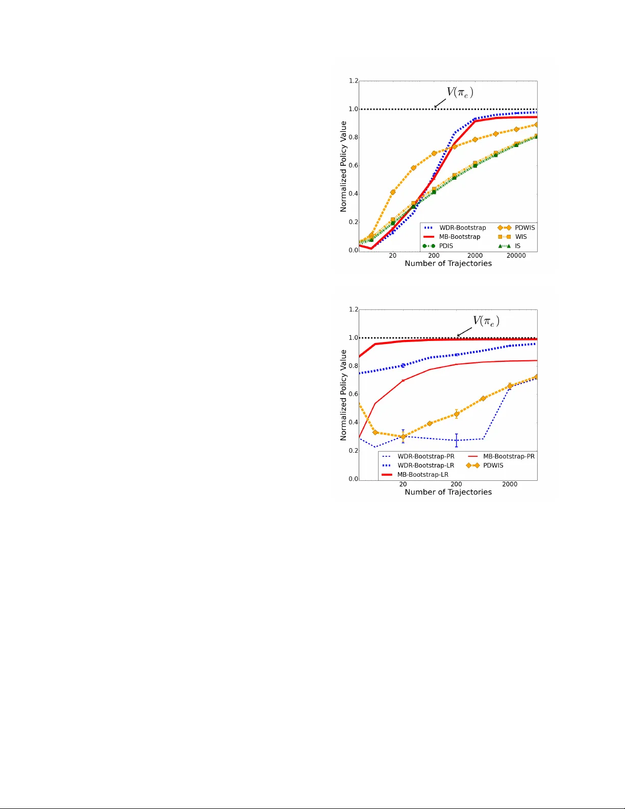
Authors: Josiah P. Hanna, Peter Stone, Scott Niekum
In Pr oceedings of the 16th International Confer ence on Autonomous Agents and Multia gent Systems (AAMAS 2017), Sao Paolo, Brazil May 2017 Bootstrapping with Models: Confidence Intervals f or Off-P olicy Ev aluation Josiah P . Hanna 1 , Peter Stone 1 , and Scott Niekum 1 1 Department of Computer Science, The Univ ersity of T exas at Austin, Austin, T exas, U.S.A ABSTRA CT For an autonomous agent, executing a poor policy may be costly or even dangerous. For such agents, it is desirable to determine confidence interval lower bounds on the performance of any gi ven policy without executing said policy . Current methods for exact high confidence off-polic y ev aluation that use importance sampling require a substantial amount of data to achie ve a tight lower bound. Existing model-based methods only address the problem in discrete state spaces. Since exact bounds are intractable for man y domains we trade off strict guarantees of safety for more data-efficient ap- proximate bounds. In this context, we propose two bootstrapping off-polic y ev aluation methods which use learned MDP transition models in order to estimate lower confidence bounds on polic y per- formance with limited data in both continuous and discrete state spaces. Since direct use of a model may introduce bias, we deriv e a theoretical upper bound on model bias for when the model transition function is estimated with i.i.d. trajectories. This bound broadens our understanding of the conditions under which model-based meth- ods hav e high bias. Finally , we empirically e valuate our proposed methods and analyze the settings in which different bootstrapping off-polic y confidence interval methods succeed and f ail. K eywords Reinforcement learning; Off-polic y ev aluation; Bootstrapping 1. INTR ODUCTION As r einfor cement learning (RL) agents find application in the real world, it will be critical to establish the performance of policies with high confidence before they are e xecuted. For example, deploying a poorly performing polic y on a manufacturing robot may slow production or , in the worst case, damage the robot or harm humans working around it. It is insufficient to ha ve a policy that has a high off-polic y predicted value — we want to specify a lower bound on the policy’ s v alue that is correct with a pre-determined lev el of confidence. This problem is known as the high confidence off- policy evaluation pr oblem . W e propose data-efficient approximate solutions to this problem. High confidence off-policy model-based methods require large amounts of data and are limited to discrete settings [4]. In con- tinuous settings, current methods for high confidence off-polic y ev aluation rely on importance sampling [13] with existing domain Appears in: Pr oceedings of the 16th International Confer ence on Autonomous Agents and Multia gent Systems (AAMAS 2017), S. Das, E. Durfee, K. Larson, M. W inikoff (eds.), May 8–12, 2017, São P aulo, Brazil. Copyright c 2017, International Foundation for Autonomous Agents and Multiagent Systems (www .ifaamas.org). All rights reserved. data [17]. Due to the large v ariance of importance sampled returns, these algorithms can require prohibiti vely large amounts of data to produce meaningful confidence bounds. The current state-of-the-art for high confidence off-polic y ev aluation in discrete and continuous settings is a concentration inequality tailored to the distrib ution of importance sampled returns [17]. Unfortunately , the amount of data required for tight confidence bounds preclude the use of this method in data-scarce settings such as robotics. Instead of e xact high confidence, Thomas et al. [18] demonstrated that approximate bounds obtained by bootstrapping importance sampled policy returns can improve data-ef ficiency by an order of magnitude over concentration inequalities. In this work, we propose two approximate high confidence off-polic y e valuation methods through the combination of bootstrapping with learned models of the environment’ s transition dynamics. Both methods are straightforward to implement (though seemingly nov el) and are empirically demonstrated to outperform importance-sampling methods. Our first contribution, Model-based Bootstrapping ( M B - B O OT S T R A P ), directly combines bootstrapping with learned models of the en vironment’ s dynamics for of f-policy value estimation. Since M B - B O O T S T R A P uses direct model-based estimates of policy value, it may exhibit bias in some settings. T o characterize these settings, we deriv e an upper bound on model bias for models estimated from arbitrary distributions of trajectories. Our second algorithmic contri- bution, weighted doubly r obust bootstrapping ( W D R - B O OT S T R A P ), combines bootstrapping with the recently proposed weighted dou- bly robust estimator [20] which uses a model to lo wer the v ariance of importance sampling estimators without adding model bias to the estimate. W e empirically evaluate both methods on two high confidence off-polic y ev aluation tasks. Our results show these meth- ods are far more data-efficient than existing importance sampling based approaches. Finally , we combine theoretical and empirical re- sults to make specific recommendations about when to use different off-polic y confidence bound methods in practice. 2. PRELIMINARIES 2.1 Marko v Decision Processes W e formalize our problem as a Marko v decision pr ocess (MDP) defined as ( S , A , P, r , γ , d 0 ) where S is a set of states, A is a set of actions, P : S × A × S → [0 . 1] is a probability mass function defining a distribution ov er next states for each state and action, r : S × A → [0 , r max ] is a bounded, non-negativ e reward function, γ ∈ [0 , 1] is a discount factor , and d 0 is a probability mass function ov er initial states. An agent samples actions from a policy , π : S × A → [0 , 1] , which is a probability mass function on A conditioned on the current state. A policy is deterministic if π ( a | s ) = 1 for only one a in each s . 1 A trajectory , H of length L is a state-action history , S 0 , A 0 , . . . , S L − 1 , A L − 1 where S 0 ∼ d 0 , A t ∼ π ( ·| s t ) , and S t +1 ∼ P ( ·| S t , A t ) . The return of a trajectory is g ( H ) = P L − 1 t =0 γ t r ( S t , A t ) . The policy , π , and transition dynamics, P , induce a distribution over trajectories, p π . W e write H ∼ π to denote a trajectory sampled by executing π (i.e., sampled from p π ). The expected discounted return of a policy , π , is defined as V ( π ) := E H ∼ π [ g ( H )] . Giv en a set of n trajectories, D = { H 1 , .., H n } , where H i ∼ π b for some behavior policy , π b , an ev aluation polic y , π e , and a confidence lev el, δ ∈ [0 , 1] , we propose tw o methods to approximate a confidence lower bound, V δ ( π e ) , on V ( π e ) such that V δ ( π e ) ≤ V ( π e ) with probability at least 1 − δ . 2.2 Importance Sampling W e define an off-policy estimator as any method for comput- ing an estimate, b V ( π e ) , of V ( π e ) using trajectories from a sec- ond policy , π b . Importance sampling ( I S ) is one such method [13]. For a trajectory H ∼ π b , where H = S 1 , A 1 , . . . , S L , A L , we define the importance weight up to time t for polic y π e as ρ H t := Q t i =0 π e ( A i | S i ) π b ( A i | S i ) . Then the I S estimator of V ( π e ) with a trajectory , H ∼ π b is defined as I S ( π e , H , π b ) := g ( H ) ρ H L . A lower variance v ersion of importance sampling for of f-policy e val- uation is per-decision importance sampling , P D I S ( π e , H , π b ) := P L − 1 t =0 r ( S t , A t ) ρ H t . W e overload I S notation to define the batch I S estimator for a set of n trajectories, D , so that I S ( D ) := 1 n P n i =1 I S ( π e , H i , π b ) . The batch P D I S estimator is defined similarly . The v ariance of batch I S estimators can be reduced with weighted importance sampling ( W I S ) and per-decision weighted importance sampling ( P D W I S ). Define the weighted importance weight up to time t for the i th trajectory as w H i t := ρ H i t / P n j =1 ρ H j t . Then the W I S estimator is defined as: W I S ( D ) := P n i =1 g ( H i ) w H i L . P D W I S is defined as P D I S with w H i t replacing ρ H i t . Provided the support of π e is a subset of the support of π b , I S and P D I S are unbiased but potentially high variance estimators. W I S and P DW I S have less variance than their unweighted counterparts but introduce bias. When all H i ∈ D are sampled from the same policy , π b , W I S and P DW I S introduce a particular form of bias. Namely , when n = 1 , b V ( π e ) is an unbiased estimate of V ( π b ) . As n increases, the estimate shifts from V ( π b ) tow ards V ( π e ) . Thus, W I S and P D W I S are statistically consistent (i.e., W I S ( D ) → V ( π e ) as n → ∞ ) [19]. 2.3 Bootstrapping This section gi ves an ov erview of bootstrapping [7]. In the next section we propose bootstrapping with learned models to estimate confidence intervals for of f-policy estimates. Consider a sample X of n random variables X i for i = 1 , . . . , n , where we sample X i i.i.d. from some distribution f . From the sample, X , we can compute a sample estimate, ˆ θ of a parameter, θ such that ˆ θ = t ( X ) . For example, if θ is the population mean, then t ( X ) := 1 n P n i =1 X i . For a finite sample, we would like to specify the accuracy of ˆ θ without placing restrictiv e assumptions on the sampling distribution of ˆ θ (e.g., assuming ˆ θ is distributed normally). Bootstrapping allo ws us to estimate the distribution of ˆ θ from whence confidence intervals can be deri ved. Starting from a sample X = { X 1 , . . . , X n } , we create B new samples, 1 W e define notation for discrete MDPs, howe ver , all results hold for continuous S and A by replacing summations with inte grals and probability mass functions with probability density functions. Algorithm 1 Bootstrap Confidence Interval Input is an evaluation policy π e , a data set of trajectories, D , a confidence lev el, δ ∈ [0 , 1] , and the required number of bootstrap estimates, B . input π e , D , π b , δ , B output 1 − δ confidence lower bound on V ( π e ) . 1: for all i ∈ [1 , B ] do 2: ˜ D i ← { H i 1 , . . . , H i n } where H i j ∼ U ( D ) // where U is the uniform distribution 3: b V i ← Off-PolicyEstimate( π e , ˜ D i , π b ) 4: end for 5: sort ( { b V i | i ∈ [1 , B ] } ) // Sort ascending 6: l ← b δ B c 7: Return b V l ˜ X j = { ˜ X j 1 , . . . , ˜ X j n } , by sampling ˜ X j i from a bootstrap distribu- tion, ˆ f . That is, we sample ˆ f by independently sampling X i from X with replacement . F or each ˜ X j we compute ˆ θ j = t ( ˜ X j ) . The distribution of the ˆ θ j approximates the distribution of ˆ θ which al- lows us to compute sample confidence bounds. See the work of Efron [6] for a more detailed introduction to bootstrapping. While bootstrapping has strong guarantees as n → ∞ , boot- strap confidence interv als lack finite sample guarantees. Using bootstrapping requires the assumption that the bootstrap distribu- tion is representativ e of the distribution of the statistic of interest which may be false for a finite sample. Therefore, we characterize bootstrap confidence intervals as “semi-safe" due to this possibly false assumption. In contrast to lower bounds from concentration inequalities, bootstrapped lower bounds can be thought of as ap- proximating the allow able δ error rate instead of upper bounding it. Howe ver , bootstrapping is considered safe enough for high risk medical predictions and in practice has a well established record of producing accurate confidence intervals [3]. In the context of policy ev aluation, Thomas et al. [18] established that bootstrap confidence intervals with W I S can provide accurate lower bounds in the high confidence of f-policy ev aluation setting. The primary contribution of our work is to incorporate off-policy estimators of V that use models into bootstrapping to decrease the data requirements needed to produce a tight lower bound. 3. OFF-POLICY BOO TSTRAPPED LO WER BOUNDS In this section, we propose model-based and weighted doubly ro- bust bootstrapping for estimating confidence interv als on off-polic y estimates. First, we present pseudocode for computing a bootstrap confidence lower bound for an y off-polic y estimator (Algorithm 1). Our proposed methods are instantiations of this general algorithm. W e define Off-PolicyEstimate to be any method that takes a data set of trajectories, D , the policy that generated D , π b , and a policy , π e , and returns a policy v alue estimate, b V ( π e ) , (i.e., an of f- policy estimator). Algorithm 1 is a Bootstrap Confidence Interval procedure in which b V ( π e ) , as computed by Off-PolicyEstimate , is the statistic of interest ( ˆ θ in Section 2.3). W e give pseudocode for a bootstrap lower bound. The method is equally applicable to upper bounds and two-sided interv als. The bootstrap method we present is the percentile bootstrap for confidence le vels [2]. A more sophisticated bootstrap approach is Bias Corrected and Accelerated bootstrapping (BCa) which ad- justs for the ske w of the distrib ution of b V i . When using I S as Off-PolicyEstimate , BCa can correct for the hea vy upper tailed distribution of I S returns [18]. 2 3.1 Direct Model-Based Bootstrapping W e no w introduce our first algorithmic contribution—model- based bootstrapping ( M B - B O O T S T R A P ). The model-based off-polic y estimator , M B , computes b V ( π e ) by first using all trajectories in D to build a model c M = ( S , A , b P , r, γ , ˆ d 0 ) where b P and ˆ d 0 are estimated from trajectories sampled i.i.d. from π b . 3 Then M B estimates b V ( π e ) as the average return of trajectories simulated in c M while follo wing π e . Algorithm 1 with the off-polic y estimator M B as Off-PolicyEstimate defines M B - B O OT S T R A P . If a model can capture the true MDP’ s dynamics or generalize well to unseen parts of the state-action space then M B estimates can have much lower variance than I S estimates. Thus we expect less variance in our b V i estimates in Algorithm 1. Howev er , models reduce variance at the cost of adding bias to the estimate. Bias in the M B estimate of V ( π e ) arises from two sources: 1. When we lack data for a particular ( s, a ) pair , we must make assumptions about how to estimate P ( ·| s, a ) . 2. If we use function approximation, we assume the model class from which we select b P includes the true transition model, P . When P is outside the chosen model class then M B ( D ) can be biased because M B ( D ) − V ( π e ) → b for some constant b 6 = 0 as n → ∞ . The first source of bias is dependent on what modeling assump- tions are made. Using assumptions which lead to more conservativ e estimates of V ( π e ) will, in practice, prev ent M B - B O OT S T R A P from ov erestimating the lower bound. The second source of bias is more problematic since even as n → ∞ the bootstrap model estimates will conv erge to a different value from V ( π e ) . In the next section we propose bootstrapping with the recently proposed weighted doubly- robust estimator in order to obtain data-efficient lower bounds in settings where model bias may be large. Later we will present a ne w theoretical upper bound on model bias when b P is learned from a dataset of i.i.d. trajectories. This bound characterizes MDPs that are likely to produce high bias estimates. 3.2 W eighted Doubly Robust Bootstrapping W e also propose weighted doubly r obust bootstrapping ( W D R - bootstrap) which combines bootstrapping with the recently proposed W D R off-polic y estimator for settings where the M B estimator may exhibit high bias. The W D R estimator is based on per-decision weighted importance sampling ( P D W I S ) but uses a model to reduce variance in the estimate. The doubly r obust ( D R ) estimator has its origins in bandit problems [5] but w as extended by Jiang and Li [10] to finite horizon MDPs. Thomas and Brunskill [20] then extended D R to infinite horizon MDPs and combined it with weighted I S weights to produce the weighted DR estimator . Given a model and its state and state-action value functions for π e , ˆ v π e and ˆ q π e , the W D R estimator is defined as: W D R ( D ):= P DW I S ( D ) − n X i =1 L − 1 X t =0 γ t ( w i t ˆ q π e ( S i t , A i t ) − w i t − 1 ˆ v π e ( S i t )) | {z } Control V ariate Term 2 If the W I S estimator is used for Off-PolicyEstimate then Algo- rithm 1 describes a simplified version of the bootstrapping method presented by Thomas et al. [18]. 3 The re ward function, r , may be approximated as ˆ r . Our theoretical results assume r is known b ut our proposed methods are applicable when this assumption fails to hold. where w − 1 := 1 . For W D R , the model value-functions are used as a control variate on the higher variance P D W I S expectation. The con- trol variate term has e xpectation zero and thus W D R is an unbiased estimator of P D W I S which is a statistically consistent estimator of V ( π e ) . Intuitiv ely , W D R uses information from error in estimating the expected return under the model to lower the variance of the P D W I S return. W e refer the reader to Thomas and Brunskill [20] and Jiang and Li [10] for an in-depth discussion of the W D R and D R estimators. Since W D R estimates of V ( π e ) hav e been shown to achiev e lower mean squared error (MSE) than those of DR in sev eral domains, we propose W D R - B O O T S T R A P which uses W D R as Off-PolicyEstimate in Algorithm 1. Although W D R is biased (since P D W I S is biased), the statistical consistency property of P DW I S ensures that the bootstrap estimates of W D R - B O O T S T R A P will conv erge to the correct estimate as n increases. Thus it is free of out-of-class model bias as n → ∞ . Empirical results have shown that W D R can achei ve lower MSE than M B in domains where the model conv erges to an incorrect model [20]. Howe ver , Thomas and Brunskill also demonstrated situations where the MB e valuation is more efficient at acheiving low MSE than W D R when the variance of the P DW I S weights is high. W e empirically analyze the trade-offs when using these estimators with bootstrapping for off-polic y confidence bounds. Note that W D R - B O OT S T R A P has three options for the model used to estimate the control variate: the model can be provided (for instance a domain simulator), the model can be estimated with all of D and this model be used with WD R to compute each b V i , or we can build a ne w model for e very bootstrap data set, D i , and use it to compute W D R for D i . In practice, an a priori model may be unav ailable and it may be computationally e xpensiv e to build a model and find the value function for that model for each bootstrap data set. Thus, in our experiments, we estimate a single model with all trajectories in D . W e use the v alue functions of this single model to compute the W D R estimate for each D i . 4. TRAJECTOR Y B ASED MODEL BIAS W e now present a theoretical upper bound on bias in the model- based estimate of V ( π e ) . Theorem 1 bounds the error of b V ( π e ) produced by a model, c M , as a function of the accuracy of c M . This bound provides insight into the settings in which M B - B O O T S T R A P is likely to be unsuccessful. The bound is related to other model bias bounds in the literature and we discuss these in our surv ey of related work. W e defer the full deri vation to Appendix A. F or this section we introduce the additional assumption that L is finite. All methods proposed in this paper are applicable to both finite and infinite horizon problems, ho wev er the bias upper bound is currently limited to the episodic finite horizon setting. T H E O R E M 1. F or any policies, π e and π b , let p π e and p π b be the distributions of trajectories induced by eac h policy . Then for an appr oximate model, c M , with transition pr obabilities estimated fr om i.i.d. trajectories H ∼ π b , the bias of b V ( π e ) is upper bounded by: b V ( π e ) − V ( π e ) ≤ 2 L · r max s 2 E H ∼ π b ρ H L log p π e ( H ) ˆ p π e ( H ) wher e ρ H L is the importance weight of trajectory H at step L and ˆ p π e is the distribution of tr ajectories induced by π e in c M . The expectation is the importance-sampled Kullbac k-Leibler (KL) div ergence. The KL-diver gence is an information theoretic measure that is frequently used as a similarity measure between probabil- ity distributions. This result tells us that the bias of M B depends on how different the distribution of trajectories under the model is from the distribution of trajectories seen when e xecuting π in the true MDP . Since most model building techniques (e.g., super- vised learning algorithms, tabular methods) build the model from ( s t , a t , s t +1 ) transitions ev en if the transitions come from sampled trajectories (i.e., non i.i.d. transitions), we express Theorem 1 in terms of transitions: C O R O L L A RY 1. F or any policies π e and π b and an appr oximate model, c M , with transition pr obabilities, b P , estimated with trajec- tories H ∼ π b , the bias of the approximate model’s estimate of V ( π e ) , b V ( π e ) , is upper bounded by: | b V ( π e ) − V ( π e ) | ≤ 2 √ 2 L · r max v u u t 0 + L − 1 X t =1 E S t ,A t ∼ d t π b [ ρ H t ( S t , A t )] wher e d t π b is the distribution of states and actions observed at time t when e xecuting π b in the true MDP , 0 := D K L ( d 0 || ˆ d 0 ) , and ( s, a ) = D K L ( P ( ·| s, a ) || b P ( ·| s, a ))) . Since P is unknown it is impossible to estimate the D K L terms in Corollary 1. Howe ver , D K L can be approximated with two common supervised learning loss functions: negativ e log likelihood and cross- entropy . W e can express Corollary 1 in terms of either negati ve log-likelihood (a regression loss function for continuous MDPs) or cross-entropy (a classification loss function for discrete MDPs) and minimize the bound with observed ( s t , a t , s t +1 ) transitions. In the case of discrete state-spaces this approximation upper bounds D K L . In continuous state-spaces the approximation is correct within the average differential entropy of P which is a problem-specific constant. Both Theorem 1 and Corollary 1 can be extended to finite sample bounds using Hoeffding’ s inequality (see Appendix A). Corollary 1 allows us to compute the upper bound proposed in Theorem 1. Howev er in practice the dependence on the maximum rew ard makes the bound too loose to subtract off from the lower bound found by M B - B O OT S T R A P . Instead, we observe it char- acterizes settings where the M B estimator may exhibit high bias. Specifically , a M B estimate of V ( π e ) will have lo w bias when we build a model which obtains lo w training error under the negati ve log-likelihood or cross-entrop y loss functions where the error due to each ( s t , a t , s t +1 ) is importance-sampled to correct for the dif fer- ence in distribution. This result holds regardless of whether or not the true transition dynamics are representable by the model class. 5. EMPIRICAL RESUL TS W e now e valuate M B - B O O T S T R A P and W D R - B O O T S T R A P across two policy e v aluation domains. 5.1 Experimental Domains The first domain is the standard MountainCar task from the RL literature [16]. In this domain an agent attempts to dri ve an under - powered car up a hill. The car cannot drive straight up the hill and a successful policy must first mov e in rev erse up another hill in order to gain momentum to reach its goal. States are discretized horizontal position and velocity and the agent may choose to accelerate left, right, or neither . At each time-step the reward is − 1 except for in a terminal state when it is 0 . W e build models as done by Jiang and Li [10] where a lack of data for a ( s, a ) pair causes a deter - ministic transition to s . Also, as in previous work on importance sampling, we shorten the horizon of the problem by holding action a t constant for 4 updates of the en vironment state [10, 19]. This Figure 1: CliffW orld domain in which an agent (A) must mov e between or around cliffs to reach a goal (G). modification changes the problem horizon to L = 100 and is done to reduce the v ariance of importance-sampling. Policy π b chooses actions uniformly at random and π e is a sub-optimal polic y that solves the task in approximately 35 steps. In this domain we b uild tabular models which cannot generalize from observed ( s, a ) pairs. W e compute the model action v alue function, ˆ q π e , and state v alue function, ˆ v π e with value-iteration for W D R . W e use Monte Carlo rollouts to estimate b V with M B . Our second domain is a continuous two-dimensional CliffW orld (depicted in Figure 1) where a point mass agent na vigates a series of cliffs to reach a goal, g . An agent’ s state is a four dimensional vector of horizontal and v ertical position and velocity . Actions are acceleration values in the horizontal and vertical directions. The rew ard is negati ve and proportional to the agent’ s distance to the goal and magnitude of the actions taken, r ( S t , A t ) = || S t − g || 1 + || A t || 1 . If the agent falls off a cliff it receiv es a large negati ve penalty . In this domain, we hand code a deterministic policy , π d . Then the agent samples π e ( ·| s ) by sampling from N ( a | π d ( s ) , Σ) . The behavior polic y is the same except Σ has greater variance. Domain dynamics are linear with additiv e Gaussian noise. W e build models in two ways: linear regression (conv erges to true model as n → ∞ ) and regression ov er nonlinear polynomial basis functions. 4 The first model class choice represents the ideal case and the second is the case when the true dynamics are outside the learnable model class. Our results refer to M B - B O O T S T R A P LR and M B - B O OT S T R A P PR as the M B estimator using linear regression and polynomial regression respectiv ely . These dynamics mean that the bootstrap models of MB-Bootstrap LR and WDR-Bootstrap LR will quickly conv erge to a correct model as the amount of data increases since they build models with linear regression. On the other hand, these dynamics mean that the models of MB-Bootstrap PR and WDR-Bootstrap PR will quickly con verge to an incorrect model since they use re gression ov er nonlinear polynomial basis functions. Similarly , we ev aluate W D R - B O OT S T R A P LR and W D R - B O OT S T R A P PR . In each domain, we estimate a 95% confidence lo wer bound ( δ = 0 . 05 ) with our proposed methods and the importance sampling BCa-bootstrap methods from Thomas et. al. [18]. T o the best of our kno wledge, these I S methods are the current state-of-the-art for approximate high confidence of f-policy ev aluation. W e use B = 2000 bootstrap estimates, b V i and compute the true value of V ( π e ) with 1,000,000 Monte Carlo roll-outs of π e in each domain. For each domain we computed the lower bound for n trajectories where n varied logarithmically . For each n we generate a set of n trajectories m times and compute the lower bound with each method (e.g., MB, WDR, IS) on that set of trajectories. For Mountain Car m = 400 and for Clif fW orld m = 100 . The large number of trials is required for the empirical error rate calculations. When plotting the average lower bound across methods, we only a verage valid lower bounds (i.e., b V δ ( π e ) ≤ V ( π e ) ) because in valid lo wer bounds 4 For each state feature, x , we include features 1 , x 2 , x 3 but not x . raise the av erage which can make a method appear to produce a tighter av erage lower bound when it fact it has a higher error rate. As in prior work [17], we normalize returns for I S and rewards for P D I S to be between [0 , 1] . Normalizing reduces the v ariance of the I S estimator . More importantly , it improves safety . Since the majority of the importance weights are close to zero, when the minimum return is zero, I S tends to underestimate policy value. Pre- liminary experiments sho wed without normalization, bootstrapping with I S resulted in ov er confident bounds. Thus, we normalize in all experiments. 5.2 Empirical Results Figure 2 displays the av erage empirical 95% confidence lower bound found by each method in each domain. The ideal result is a lower bound, V δ ( π e ) , that is as large as possible subject to V δ ( π e ) < V ( π e ) . Given that an y statistically consistent method will achie ve the ideal result as n → ∞ , our main point of comparison is which method gets closest the f astest. As a general trend we note that our proposed methods— M B - B O O T S T R A P and W D R - B O OT S T R A P — get closer to this ideal result with less data than all other methods. Figure 3 displays the empirical error rate for M B - B O O T S T R A P and W D R - B O OT S T R A P and shows that they approximate the allo wable 5% error in each domain. In MountainCar (Figure 2a), both of our methods ( W D R - B O O T S T R A P and M B - B O O T S T R A P ) outperform purely I S methods in reaching the ideal result. W e also note that both methods produce approximately the same average lower bound. The modelling as- sumption that lack of data for some ( s, a ) results in a transition to s is a form of negati ve model bias which lowers the performance of M B - B O O T S T R A P . Therefore, e ven though M B will eventually con ver ge to V ( π e ) it does so no faster than W D R which can produce good estimates even when the model is inaccurate. This negati ve bias also leads to P D W I S producing a tighter bound for small data sets although it is overtak en by M B - B O OT S T R A P and W D R - B O OT S T R A P as the amount of data increases. Figure 3a sho ws that the M B - B O OT S T R A P and W D R - B O O T S T R A P error rate is much lower than the required error rate yet Figure 2a shows the lower bound is no looser . Since M B - B O O T S T R A P and W D R - B O OT S T R A P are low v ariance estimators, the av erage bound can be tight with a low error rate. It is also notable that since bootstrapping only approximates the 5% allo wable error rate all methods can do worse than 5% when data is extremely sparse (only two trajectories). In Cliff W orld (Figure 2b), we first note that M B - B O OT S T R A P PR quickly con verges to a suboptimal lo wer bound. In practice an incorrect model may lead to a bound that is too high (positi ve bias) or too loose (negativ e bias). Here, M B - B O O T S T R A P PR exhibits negati ve bias and we conv erge to a bound that is too loose. More dangerous is positiv e bias which will make the method unsafe. Our theoretical results suggest M B bias is high when ev aluating π e since the polynomial basis function models have high training error when errors are importance-sampled to correct for the off-policy model estimation. If we compute the bound in Section 4 and subtract the value of f from the bound estimated by M B - B O O T S T R A P PR then the lower bound estimate will be unaf fected by bias. Unfortunately , our theoretical bound (and other model-bias bounds in earlier work) depends on the lar gest possible return, L · r max and thus removing bias in this straightforward way reduces data-ef ficiency gains when bias may in fact be much lo wer . The second notable trend is that W D R is also negati vely im- pacted by the incorrect model. In Figure 2b we see that W D R - B O O T S T R A P LR (correct model) starts at a tight bound and increases from there. WD R - B O O T S T R A P PR with an incorrect model performs (a) Mountain Car (b) CliffW orld Figure 2: The average empirical lower bound for the Mountain Car and CliffW orld domains. Each plot displays the 95% lower bound on V ( π e ) computed by each method with v arying amounts of trajectories. The ideal lower bound is just belo w the line labelled V ( π e ) . Results demonstrate that the proposed model-based bootstrapping ( M B - B O O T S T R A P ) and weighted doubly robust bootstrapping ( W D R - B O OT S T R A P ) find a tighter lower bound with less data than previous importance sampling bootstrapping methods. For clarity , we omit I S , W I S and P D I S in CliffW orld as they were outperformed by P D W I S . Error bars are for a 95% two-sided confidence interval. worse than P DW I S until larger n . Using an incorrect model with W D R decreases the variance of the P D W I S term less than the correct model would but we still expect less variance and a tighter lower bound than P D W I S by itself. One possibility is that error in the esti- mate of the model value functions coupled with the inaccurate model increases the v ariance of W D R . This result motiv ates inv estigating the ef fect of inaccurate model state-v alue and state-action-value functions on the W D R control variate as these functions are certain to hav e error in any continuous setting. (a) Mountain Car (b) CliffW orld Figure 3: Empirical error rate for the Mountain Car and CliffW orld do- mains. The lower bound is computed m times for each method ( m = 400 for Mountain Car , m = 100 for CliffW orld) and we count how many times the lo wer bound is above the true V ( π e ) . All methods correctly approximate the allow able 5% error rate for a 95% confidence lo wer bound. 6. RELA TED WORK Concentration inequalities ha ve been used with I S returns for lower bounds on off-polic y estimates [17]. The concentration in- equality approach is notable in that it produces a true probabilistic bound on the policy performance. A similar b ut approximate method was proposed by Bottou et al [1]. Unfortunately , these approachs requires prohibitiv e amounts of data and were sho wn to be far less data-efficient than bootstrapping with I S [18, 19]. Jiang and Li ev aluated the DR estimator for safe-policy improv ement [10]. They compute confidence intervals with a method similar to the Student’ s t -T est confidence interval sho wn to be less data-efficient than boot- strapping [18]. Chow et al. [4] use ideas from robust optimization to deriv e a lower bound on V ( π e ) by first bounding model bias caused by error in a discrete model’ s transition function. This bound is computable only if the error in each transition can be bounded and is inappli- cable for estimating bias in continuous state-spaces. Model-based P AC-MDP methods can be used to synthesize policies which are approximately optimal with high probability [8]. These methods are only applicable to discrete MDPs and require large amounts of data. Other bounds on the error in estimates of V ( π ) with an inaccurate model hav e been introduced for discrete MDPs [11, 15]. In contrast, we present a bound on model bias that is computable in both continu- ous and discrete MDPs. Ross and Bagnell introduce a bound similar to Corollary 2 for model-based policy improv ement but assume that the model is estimated from transitions sampled i.i.d. from a gi ven exploration distrib ution [14]. Since we bootstrap ov er trajectories their bound is inapplicable to our setting. Paduraru introduced tight model bias bounds for i.i.d. sampled transitions from general MDPs and i.i.d. trajectories from directed acyclic graph MDPs [12]. W e made no assumptions on the structure of the MDP when deriving our bound. Other pre vious work has used bootstrapping to handle uncertainty in RL. The T E X P L O R E algorithm learns multiple decision tree mod- els from subsets of experience to represent uncertainty in model predictions [9]. White and White [21] use time-series bootstrapping to place confidence intervals on value-function estimation during policy learning. Thomas and Brunskill introduce an estimate of the model-based estimator’ s bias using a combination of W D R and bootstrapping [20]. While these methods are related through the combination of bootstrapping and RL, none address the problem of confidence intervals for of f-policy e valuation. 7. DISCUSSION W e have proposed two bootstrapping methods that incorporate models to produce tight lo wer bounds on of f-policy estimates. W e now describe their advantages and disadvantages and make recom- mendations about their use in practice. Model-based Bootstrapping. Clearly , M B - B O OT S T R A P is influenced by the quality of the es- timated transition dynamics. If M B - B O O T S T R A P can build models with low importance-sampled approximation error then we can expect it to be more data-efficient than other methods. This data- efficienc y comes at a cost of potential bias. Our theoretical results show that bias is una voidable for some model-class choices. How- ev er if the chosen model-class can be learned with low approxi- mation error on D then model bias will be low . In practice model prediction error for of f-policy ev aluation may be e valuated with a held out subset of D (i.e., model validation error). If the model fails to generalize to unseen data then another of f-policy method is preferable. Importance-sampling the test error giv es a measure of how well a model estimated with trajectories from π b will generalize for ev aluating π e . W eighted Doubly-Robust Bootstr ap. Our proposed W D R - B O OT S T R A P method provides a low v ariance and low bias method of high confidence of f -policy ev aluation. These two properties allo w W D R - B O O T S T R A P to outperform different variants of I S and sometimes perform as well or better than M B - B O O T S T R A P . In contrast to M B - B O O T S T R A P , W D R - B O O T S T R A P achiev es data-efficient lo wer bounds while remaining free of model bias. Since W D R - B O OT S T R A P is free of model bias, it should be the preferred method if model quality is unknown or the domain is hard to model. A disadvantage of W D R - B O O T S T R A P is that it requires the model’ s value functions be known for all states and state-action pairs that occur along trajectories in D . In continuous state and action spaces this requires either function approximation or Monte Carlo e val- uation. The variance of either method can increase the variance of the W D R estimate. Note that W D R remains bias free provided ˆ v π e ( s ) = E A ∼ π e ( ·| s ) [ ˆ q π e ( s, A )] which ensures the control variate term has expected v alue zero ev en if ˆ q π e is a biased estimate of the policy’ s action value function under the model. A second limitation of W D R is that it biases b V ( π e ) tow ards V ( π b ) when the trajectory dataset is small. This bias is problematic for confidence bounds when V ( π b ) > V ( π e ) as the lower bound on V ( π e ) will exhibit positiv e bias. While the bias is a problem for general high confidence of f-policy ev aluation it is harmless in the specific case of high confidence off-policy improvement. In this setting the purpose of the test is to decide if we are confident that the ev aluation policy is better than the behavior policy . If in fact V ( π b ) > V ( π e ) the lo wer bound will still be less than V ( π b ) and an unsafe polic y improvement step is av oided. Similarly , if we know V ( π b ) > V ( π e ) than W D R - B O OT S T R A P will likely hav e less variance than I S -based methods and less bias than M B - B O O T S T R A P . Importance Sampling Methods. For general high confidence of f-policy e valuation tasks in which model estimation error is high, I S - or P D I S -based bootstrapping provides the safest approximate high confidence of f-policy ev alua- tion method. W e have noted that normalizing returns and re wards is an important factor in using these methods safely . Since most importance weights are close to zero the I S estimate will be pulled tow ards zero which corresponds to underestimating value. When safety is critical, underestimating is preferable to overestimating for a lower bound. Our experiments used normalization as we found unnormalized returns have too high of variance to be used safely with bootstrapping. Finally , in settings where safety must be strictly guaranteed, con- centration inequalities with I S hav e been shown to outperform other exact methods [17]. If the data is av ailable, then exact methods are preferred for their theoretical guarantees. Special Cases. T wo special cases that occur in real world high confidence off- policy e valuation are deterministic policies and unknown π b . When π e is deterministic, one should use M B - B O OT S T R A P since the im- portance weights equal zero at any time step that π b chose action a t such that π e ( A t = a t | S t ) = 0 . Deterministic π b are problematic for any method since they produce trajectories which lack a v ariety of action selection data. W e also note that importance-sampled train- ing error for assessing model quality is inapplicable to this setting. Unknown π b occur when we hav e domain trajectories but no knowl- edge of the policy that produced the trajectories. For example, a medical domain could have data on treatments and outcomes b ut the doctor’ s treatment selection policy be unknown. In this setting, im- portance sampling methods cannot be applied and M B - B O OT S T R A P may be the only way to provide a confidence interval on a ne w policy . A current gap in the literature e xists for these special cases with unbiased bounds in continuous settings. 8. CONCLUSION AND FUTURE WORK W e hav e introduced two straightforward yet novel methods— M B - B O O T S T R A P and W D R - B O OT S T R A P —that approximate confidence intervals for of f-policy ev aluation with bootstrapping and learned models. Empirically , our methods yield superior data-efficiency and tighter lower bounds on the performance of the ev aluation policy than state-of-the-art importance sampling based methods. W e also deriv ed a ne w bound on the e xpected bias of M B when learning models that minimize error over a dataset of trajectories sampled i.i.d. from an arbitrary policy . T ogether , the empirical and theoretical results enhance our understanding of bootstrapping for off-policy confidence intervals and allo w us to make recommendations on the settings where different methods are appropriate. Our ongoing research agenda includes applying these techniques within robotics. In robotics, off-polic y challenges may arise from data scarcity , deterministic policies, or unknown beha vior policies (e.g., demonstration data). While these challenges suggest M B - B O O T S T R A P is appropriate, robots may exhibit complex, non-linear dynamics that are hard to model. Understanding and finding solu- tions for high confidence of f-policy e valuation across robotic tasks may inspire innov ation that can be applied to other domains as well. Acknowledegments W e would like to thank Phil Thomas, Matthe w Hausknecht, Daniel Brown, St efano Albrecht, and Ajinkya Jain for useful discussions and insightful comments and Emma Brunskill and Y ao Liu for point- ing out an error in an earlier version of this work. This work has taken place in the Personal Autonomous Robotics Lab (PeARL) and Learning Agents Research Group (LARG) at the Artificial In- telligence Laboratory , The University of T exas at Austin. PeARL research is supported in part by NSF (IIS-1638107, IIS-1617639). LARG research is supported in part by NSF (CNS-1330072, CNS- 1305287, IIS-1637736, IIS-1651089), ONR (21C184-01), AFOSR (F A9550-14-1-0087), Raytheon, T oyota, A T&T , and Lockheed Mar- tin. Josiah Hanna is supported by an NSF Graduate Research Fellow- ship. Peter Stone serves on the Board of Directors of, Cogitai, Inc. The terms of this arrangement have been re viewed and approv ed by the Univ ersity of T exas at Austin in accordance with its polic y on objectivity in research. A ppendices A. This appendix proves all theoretical results contained in the main text. For con venience, proofs are gi ven for discrete state and action sets. Results hold for continuous states and actions by replacing summations o ver states and actions with integrals and changing probability mass functions to probability density functions. A.1 Model Bias when Evaluation and Behav- ior Policy ar e the Same L E M M A 1. F or any policy π , let p π be the distribution of tra- jectories gener ated by π and ˆ p π be the distrib ution of trajectories generated by π in an appr oximate model, c M . The bias of an esti- mate, b V ( π ) , under c M is upper bounded by: V ( π ) − b V ( π ) ≤ 2 √ 2 L · r max p D K L ( p π || ˆ p π ) wher e D K L ( p π || ˆ p π ) is the Kullbac k-Leibler (KL) diverg ence be- tween pr obability distributions p π and ˆ p π . P R O O F . V ( π ) − b V ( π ) = X h p π ( h ) g ( h ) − X h ˆ p π ( h ) g ( h ) From Jensen’ s inequality and the fact that g ( h ) ≥ 0 : V ( π ) − b V ( π ) ≤ X h | p π ( h ) − ˆ p π ( h ) | g ( h ) After replacing g ( h ) with the maximum possible return, g max := L · r max , and f actoring it out of the summation, we can use the definition of the total variation ( D T V ( p || q ) = 1 2 X x | p ( x ) − q ( x ) | ) to obtain: V ( π ) − b V ( π ) ≤ 2 D T V ( p π || ˆ p π ) · g max The definition of g max and Pinsker’ s inequality ( D T V ( p || q ) ≤ p 2 D K L ( p || q ) ) completes the proof. A.2 Bounds in terms of beha vior policy data T H E O R E M 1. F or any policies π e and π b let p π e and p π b be the distributions of trajectories induced by each policy. Then for an appr oximate model, c M , estimated with i.i.d. trajectories, H ∼ π b , the bias of the estimate of V ( π e ) with c M , b V ( π e ) , is upper bounded by: b V ( π e ) − V ( π e ) ≤ 2 √ 2 L · r max s E H ∼ π b ρ H L log p π e ( H ) ˆ p π e ( H ) wher e ρ H L is the importance weight of trajectory H at step L and ˆ p π e is the distribution of tr ajectories induced by π e in c M . P R O O F . Theorem 1 follows from Lemma 1 with the importance- sampling identity (i.e., importance-sampling the expectation in Lemma 1 so that it is an expectation with H ∼ π b ). The transition probabilities cancel in the importance weight, p π e ( H ) p π b ( H ) , leaving us with ρ H L and completing the proof. A.3 Bounding Theorem 1 in terms of a Super - vised Loss Function W e now e xpress Theorem 1 in terms of an expectation ov er tran- sitions that occur along sampled trajectories. C O R O L L A RY 1. F or any policies π e and π b and an appr oximate model, c M , with transition pr obabilities, b P , estimated with trajec- tories H ∼ π b , the bias of the approximate model’s estimate of V ( π e ) , b V ( π e ) , is upper bounded by: | b V ( π e ) − V ( π e ) | ≤ 2 √ 2 L · r max v u u t 0 + L − 1 X t =1 E S t ,A t ∼ d t π b [ ρ H t ( S t , A t )] wher e d t π b is the distribution of states and actions observed at time t when executing π b in the true MDP , 0 := D K L ( d 0 || ˆ d 0 ) , and ( s, a ) = D K L ( P ( ·| s, a ) || b P ( ·| s, a ))) . Corollary 1 follows from Theorem 1 by equating the expectation to an expectation in terms of ( S t , A t , S t +1 ) samples: P R O O F . E H ∼ π b ρ H L log p π e ( H ) ˆ p π e ( H ) = X h p π ( h ) log p π ( h ) ˆ p ˆ π ( h ) = X s 0 X a 0 ··· X s L − 1 X a L − 1 d 0 ( s 0 ) π b ( a 0 | s 0 ) ··· P ( s L − 1 | s L − 2 , a L − 2 ) · π b ( a L − 1 | s L − 1 ) ρ H L log p ( s 0 ) · · · P ( s L − 1 | s L − 2 , a L − 2 ) ˆ p ( s 0 ) · · · b P ( s L − 1 | s L − 2 , a L − 2 ) Using the logarithm property that log( ab ) = log ( a ) + log( b ) and rearranging the summation allows us to marginalize the probabilities that do not appear in the logarithm. = X s 0 d 0 ( s 0 ) log d 0 ( s 0 ) ˆ d 0 ( s 0 ) + L − 1 X t =1 X s 0 d 0 ( s 0 ) · · X s t ρ H L P ( s t | s t − 1 , a t − 1 ) log P ( s t | s t − 1 , a t − 1 ) b P ( s t | s t − 1 , a t − 1 ) Define the probability of observing s and a at time t + 1 when following π b recursiv ely as d t +1 π b ( s, a ) := X s t ,a t d t π b ( s t , a t ) P ( s | s t , a t ) π b ( a | s ) where d 1 π b ( s, a ) := d 0 ( s ) π b ( a | s ) . Using this definition to simplify: = D K L ( d 0 || ˆ d 0 ) + L − 1 X t =1 E S,A ∼ d t π b h ρ H L D K L ( P ( ·| S, A ) || b P ( ·| S, A )) i W e relate D K L to two common supervised learning loss functions so that we can minimize Corollary 1 with ( S t , A t , S t +1 ) samples. D K L ( P || b P ) = H [ P, b P ] − H [ P ] where H [ P ] and H [ P , b P ] are entropy and cross-entropy respectiv ely . F or discrete distributions, H [ P , b P ] − H [ P ] ≤ H [ P , b P ] since entropy is al ways positiv e. This fact allo ws us to upper bound D K L with the cross-entropy loss func- tion. The cross-entropy loss function is equi valent to the e xpected negati ve log likelihood loss function: H ( P ( ·| s, a ) , b P ( ·| s, a ))) = E S 0 ∼ P ( ·| s,a ) [ − log b P ( S 0 | s, a )] = E S 0 ∼ P ( ·| s,a ) [nlh( b P , s, a, S 0 )] where nlh( P , s, a, s 0 ) := − log ( P ( s 0 | s, a )) . Thus our bound ap- plies to maximum likelihood model learning. For continuous do- mains where the transition function is a probability density function, entropy can be negati ve so the negati ve log-likelihood or cross- entropy loss functions will not always bound model bias. In this case, our bound approximates the true bias bound to within a con- stant. A.4 Finite Sample Bounds Theorem 1 can be expressed as a finite-sample bound by applying Hoeffding’ s inequality to bound the expectation in the bound. C O R O L L A RY 2. F or any policies π e and π b and an appr oxi- mate model, c M , with transition pr obabilities, b P , estimated with transitions, ( s, a ) , fr om trajectories H ∼ π b , and after observing m trajectories then with pr obability α , the bias of the appr oximate model’ s estimate of V ( π e ) , b V ( π e ) , is upper bounded by: b V ( π e ) − V ( π e ) ≤ 2 L · r max · v u u u t 2 ¯ ρ L s ln( 1 α ) 2 m − 1 m X h ∈D ρ h L log ˆ d 0 ( s 1 ) + L − 1 X t =1 log b P ( s t +1 | s t , a t ) ! wher e ¯ ρ L is an upper bound on the importance ratio, i.e ., for all ρ h L , ρ h L < ¯ ρ L . P R O O F . Corollary 2 follows from applying Hoef fding’ s Inequal- ity to Theorem 1 and then expanding D KL ( p || ˆ p ) to be in terms of samples as done in the deriv ation of Corollary 1. W e then drop logarithm terms which contain the unknown d 0 and P functions. Dropping these terms is equiv alent to expressing Corollary 2 in terms of the cross-entropy or neg ative log-lik elihood loss functions. REFERENCES [1] Léon Bottou, Jonas Peters, Joaquin Quinonero Candela, Denis Xavier Charles, Max Chick ering, Elon Portugaly , Dipankar Ray , Patrice Y Simard, and Ed Snelson. Counterfactual reasoning and learning systems: the example of computational advertising. J ournal of Machine Learning Resear ch , 14(1):3207–3260, 2013. [2] James Carpenter and John Bithell. Bootstrap confidence intervals: when, which, what? a practical guide for medical statisticians. Statistics in Medicine , pages 1141–1164, 2000. [3] Lloyd E Chambless, Aaron R Folsom, A Riche y Sharrett, Paul Sorlie, David Couper , Moyses Szklo, and F Javier Nieto. Coronary heart disease risk prediction in the atherosclerosis risk in communities (aric) study . Journal of clinical epidemiology , 56(9):880–890, 2003. [4] Y inlam Chow , Marek Petrik, and Mohammad Ghav amzadeh. Robust polic y optimization with baseline guarantees. arXiv pr eprint arXiv:1506.04514 , 2015. [5] Miroslav Dudík, John Langford, and Lihong Li. Doubly robust polic y ev aluation and learning. In Pr oceedings of the 28th International Confer ence on Machine Learning, ICML , 2011. [6] B et al. Efron. Bootstrap methods: Another look at the jackknife. The Annals of Statistics , 7(1):1–26, 1979. [7] Bradley Efron. Better bootstrap confidence interv als. Journal of the American statistical Association , 82(397):171–185, 1987. [8] Jie Fu and Ufuk T opcu. Probably approximately correct mdp learning and control with temporal logic constraints. In Pr oceedings of Robotics: Science and Systems Confer ence , 2014. [9] T odd Hester and Peter Stone. Real time targeted e xploration in large domains. In The Ninth International Confer ence on Development and Learning (ICDL) , August 2010. [10] Nan Jiang and Lihong Li. Doubly robust of f-policy ev aluation for reinforcement learning. In Pr oceedings of the 33r d International Confer ence on Machine Learning, ICML , 2015. [11] Michael Kearns and Satinder Singh. Near -optimal reinforcement learning in polynomial time. Mac hine Learning , 49(2-3):209–232, 2002. [12] Cosmin Paduraru. Of f-policy Evaluation in Markov Decision Pr ocesses . PhD thesis, McGill Univ ersity , 2013. [13] Doina Precup, Richard S. Sutton, and Satinder Singh. Eligibility traces for off-polic y policy e valuation. In Pr oceedings of the 17th International Confer ence on Machine Learning , 2000. [14] Stephane Ross and J. Andrew Bagnell. Agnostic system identification for model-based reinforcement learning. In 29th International Confer ence on Machine Learning, ICML , 2012. [15] Alexander L Strehl, Lihong Li, and Michael L Littman. Reinforcement learning in finite mdps: Pac analysis. J ournal of Machine Learning Resear ch , 10:2413–2444, 2009. [16] Richard S. Sutton and Andrew G. Barto. Reinfor cement Learning: An Intr oduction . MIT Press, 1998. [17] P . S. Thomas, Georgios Theocharous, and Mohammad Ghav amzadeh. High confidence off-polic y ev aluation. In Association for the Advancement of Artificial Intelligence, AAAI , 2015. [18] P . S. Thomas, Georgios Theocharous, and Mohammad Ghav amzadeh. High confidence policy impro vement. In Pr oceedings of the 32nd International Confer ence on Machine Learning, ICML , 2015. [19] P .S. Thomas. Safe Reinfor cement Learning . PhD thesis, Univ ersity of Massachusetts Amherst, 2015. [20] P .S. Thomas and Emma Brunskill. Data-efficient of f-policy policy e valuation for reinforcement learning. In Pr oceedings of the 33r d International Confer ence on Machine Learning, ICML , 2016. [21] Martha White and Adam White. Interval estimation for reinforcement-learning algorithms in continuous-state domains. In Advances in Neural Information Pr ocessing Systems , pages 2433–2441, 2010.
Original Paper
Loading high-quality paper...
Comments & Academic Discussion
Loading comments...
Leave a Comment