Deep Encoder-Decoder Models for Unsupervised Learning of Controllable Speech Synthesis

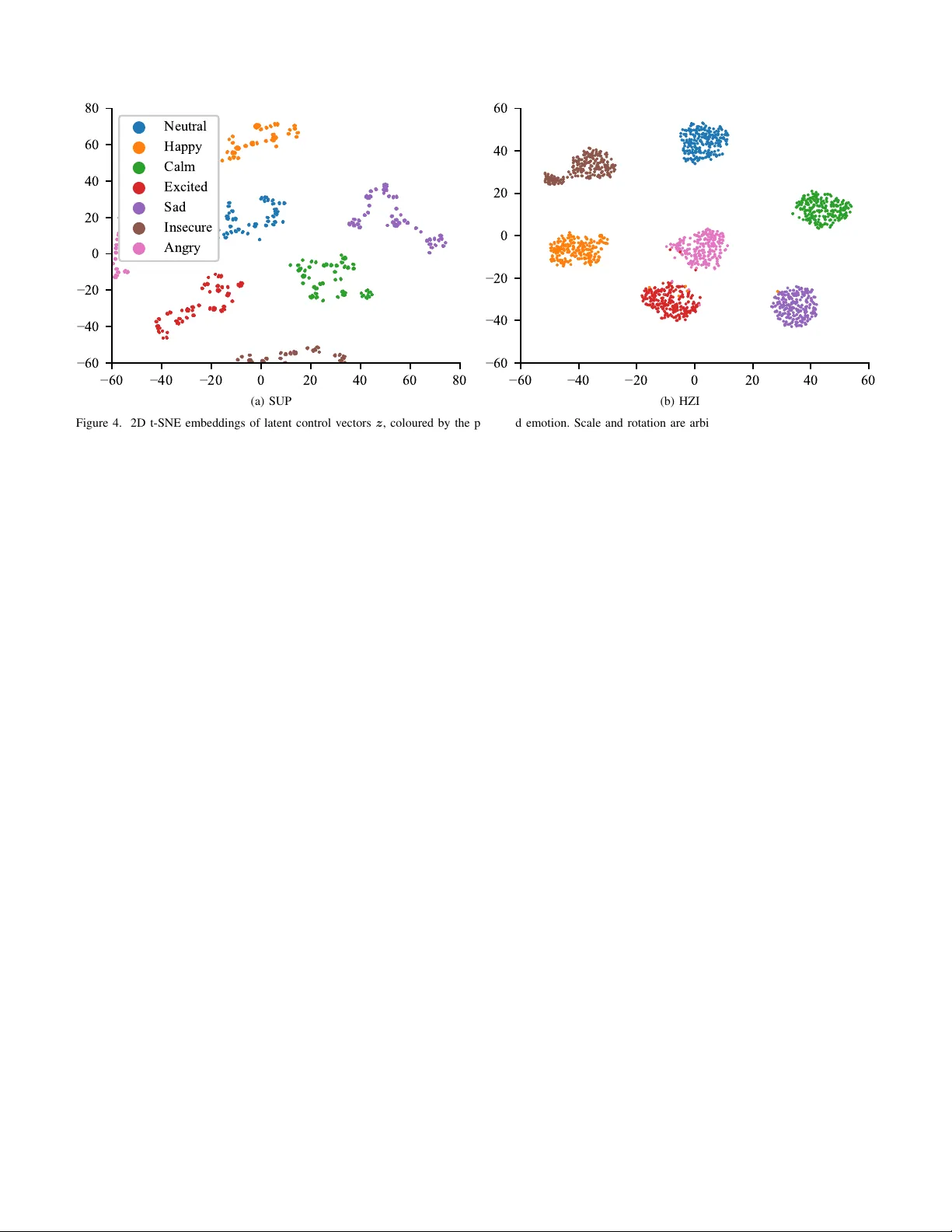
PREPRINT . WORK IN PR OGRESS. 1 Deep Encoder -Decoder Models for Unsupervised Learning of Controllable Speech Synthesis Gustav Eje Henter, Member , IEEE, Jaime Lorenzo-Trueba ‡ , Member , IEEE, Xin W ang, Student Member , IEEE, and Junichi Y amagishi, Senior Member , IEEE Abstract —Generating versatile and appr opriate synthetic speech requir es control over the output expr ession separate from the spoken text. Important non-textual speech variation is seldom annotated, in which case output control must be learned in an unsupervised fashion. In this paper , we perform an in- depth study of methods f or unsupervised learning of control in statistical speech synthesis. For example, we show that popular unsupervised training heuristics can be interpreted as variational inference in certain autoencoder models. W e additionally connect these models to VQ-V AEs, another , recently-pr oposed class of deep v ariational autoencoders, which we show can be derived from a very similar mathematical argument. The implications of these new probabilistic interpretations are discussed. W e illustrate the utility of the various approaches with an application to acoustic modelling f or emotional speech synthesis, where the unsupervised methods for learning expression control (without access to emotional labels) are found to gi ve results that in many aspects match or surpass the previous best supervised approach. Index T erms —Controllable speech synthesis, latent variable models, autoencoders, variational inference, VQ-V AE. I . I N T RO D U C T I O N T EXT to speech (TTS) is the task of turning a gi ven text into an audio wav eform of the te xt message being spoken out loud. While speech wa veforms hav e a very high bitrate (e.g., 705,600 bits per second for CD-quality audio), the spoken text only accounts for a handful of these bits, perhaps 50 or 100 bits per second [ 1 ]. A major challenge of text-to- speech synthesis is thus to ﬁll in the additional bits in the audio signal in an appropriate and con vincing manner . This is not an easy task, as speech features have complex interdependencies [ 2 ]. Furthermore, much of the excess acoustic v ariation in speech is not completely random and incidental, but con veys additional side-information of relev ance to communication. The acoustics may , for instance, reﬂect characteristics such as Manuscript last re vised July 30, 2018. This research was carried out while all authors were with the Digital Content and Media Sciences Research Division at the National Institute of Informatics, 2-1-2 Hitotsubashi, Chiyoda-ku, T okyo 101-8430, Japan. G. E. Henter is with the Department of Speech, Music and Hearing (TMH) at KTH Royal Institute of T echnology , 100 44 Stockholm, Sweden. (e-mail: ghe@kth.se ) J. Lorenzo-Trueba is with Amazon.com in Cambridge, U.K. (e-mail: jaime@nii.ac.jp ) X. W ang is with the Digital Content and Media Sciences Research Division at the National Institute of Informatics, Japan. (e-mail: wangxin@nii.ac.jp ) J. Y amagishi is with the Digital Content and Media Sciences Research Division at the National Institute of Informatics, Japan, as well as with the Centre for Speech T echnology Research at the University of Edinburgh, 10 Crichton Street, Edinb urgh EH8 9AB, U.K. (e-mail: jyamagis@nii.ac.jp ) ‡ W ork performed prior to joining Amazon. speaker identity , speak er condition, speaker mood and emo- tion, pragmatics (via emphasis and intonation), the acoustic en vironment, and properties of the communication channel (microphone characteristics, room acoustics). Neither of these are determined by the spoken text. Ideally , the acoustic cues and v ariability encountered in natural speech should not only be replicated in the acoustics to make the synthesis more con vincing, but also be adjustable to create ﬂexible and expressi ve synthesisers, and ultimately enhance communication between man and machine. Unfortu- nately , this is not the case today . Most statistical parametric speech synthesis approaches are based on supervised learn- ing, and only account for the variation that can be directly explained by the annotation provided. Any deviations from the conditional mean as predicted from annotated labels is assumed to be random and largely uncorrelated, regardless of any structure or information it may possess. At synthesis time, recreating the lost v ariability by drawing random samples from ﬁtted Gaussian models has been found to be a poor strategy from a perceptual point of view , cf. [ 3 ], wherefore the predicted average speech features are used in synthesis instead; in fact, acoustic models must be highly accurate before random sampling outperforms the av erage speech [ 2 ]. Using the model mean for synthesis makes the same utterance sound exactly identical e very time it is synthes- ised (unlike when humans speak), and is still likely to gi ve rise to artefacts, for instance widened formant bandwidths when using spectral or cepstral acoustic feature representations. In theory , salient variation beyond the text could be an- notated in the database, enabling the acoustic ef fects of the additional labels to be learned during training and controlled during synthesis. Howe ver , speech annotation is laborious, difﬁcult, and often subjectiv e. This mak es it costly to obtain sufﬁcient amounts of data where non-text variation has been annotated accurately . Instead, synthesis practise has focussed on reducing the amount of (unhandled) acoustic variability by recording TTS databases of single talkers reading text in a consistent neutral tone. The use of such data for building synthesisers may beneﬁt segmental acoustic quality , but likely contributes to the ﬂat and detached deli very that many text- to-speech systems suffer from. Se veral publications [ 4 ]–[ 7 ] hav e meanwhile highlighted the potential beneﬁts of acoustic variation (at least when annotated), for instance [ 7 ] presenting multi-speaker synthesisers that are more accurate than could be expected from training on any single speaker in the database alone and additionally allow control over properties of the generated speech, such as the speaker’ s v oice. 2 PREPRINT . WORK IN PROGRESS. This paper considers a number of alternati ves to the standard approach outlined abov e. The common theme is to in vestigate and connect methods that attempt to explicitly account for the effects of unannotated variation in the data. These methods are able to learn synthesisers with controllable output acoustics (beyond the ef fects of the input text), albeit without an a- priori labelling of the perceptual ef fects of the learned control; this can be seen as an important, though not suf ﬁcient, step to eventually enable ﬂexible speaking systems that respond appropriately to communicati ve conte xt. Mathematically , our perspectiv e is that of probabilistic modelling, speciﬁcally the theory of latent variables, and a major part of the work is to establish theoretical connections between practical approaches and principles of statistical estimation. Our main scientiﬁc contributions can be summarised as follo ws: 1) W e use v ariational methods to show that several prior methods for learning controllable models from data with unannotated variation – the training heuristic used in [ 7 ]–[ 12 ], as well as so-called VQ-V AEs from [ 13 ] – can be interpreted as approximate maximum-likelihood approaches, and elucidate the approximations in volv ed. 2) W e introduce and detail various theoretical connections between the techniques in [ 7 ], [ 10 ]–[ 12 ] and encoder- decoder models, particularly VQ-V AEs. 3) W e consider ways in which prior information can be integrated into the heuristic approaches (which lack an explicit prior distribution). 4) W e use a large database of emotional speech to perform objectiv e and subjecti ve empirical ev aluations of the heuristic approaches (with and without prior informa- tion) against comparable VQ-V AEs and a competitiv e supervised system on the task of acoustic modelling. The unsupervised methods are found to produce equal or better results than the supervised approach. These contributions all extend preliminary work performed in [ 14 ]. The remainder of this article is laid out as follows: Sec. II outlines rele vant prior work while Sec. III describes math- ematical foundations. Sec. IV then presents novel interpret- ations of and connections between different encoder -decoder approaches. Sec. V recounts empirical ev aluations performed on a database of emotional speech, while Sec. VI concludes. I I . P R I O R W O R K In this section, we introduce controllable speech synthesis (Sec. II-A ) and a wide v ariety of previous work of rele vance to our contributions. W e especially consider unsupervised learning of control (Sec. II-B ) and variational autoencoders (Sec. II-C ) and their use in speech generation (Sec. II-D ). W e also gi ve an introduction to prior work on emotional speech synthesis (Sec. II-E ), as this is the control task considered in our e xperiments. A. Controllable Speech Synthesis All text-to-speech systems are in a sense controllable, since the input text inﬂuences the output audio. (V oice con version, similarly , represents a speech synthesiser driv en by speech rather than text.) By controllable speec h synthesis , ho wever , we refer to speech synthesisers that enable additional output control beyond the words alone, such that the same te xt can be made to be spoken in se veral, perceptually distinct ways. Early , rule-based parametric speech synthesisers typically exposed many control knobs (“speech parameters”) relating to speech articulation and pronunciation; the text-to-speech aspect was simply a set of rules for how these knobs were to be moved in response to phonemes extracted from text [ 15 ], and the resulting parameter trajectories could be manually edited in order to alter pronunciation. Unit selection TTS can achiev e control of any properties annotated in the database by including a term in the tar get cost to preferentially select units with labels similar to the user-selected control input. Howe ver , success depends heavily on the database having adequate co verage of the desired control conﬁguration. W ith the transition to statistical parametric speech synthesis (SPSS), [ 16 ], [ 17 ] it became straightforward to learn to control synthesiser output, i.e., to learn a mapping from control inputs to acoustic outputs. This avoids having to design the signal generator to expose the desired speech properties to be con- trolled or manually tuning weight factors in the tar get cost, and typically achiev es meaningful control from smaller training databases than unit-selection approaches. The decision trees used in early SPSS systems can relati vely easily incorporate additional categorical labels as phone- or frame-level inputs. Continuous-valued inputs can be quantised for decision-tree learning, and the quantisation threshold can be learned as well (e.g., through C4.5 [ 18 ]). So-called multiple regression HMMs (MR-HMMs) [ 19 ] were developed as a more reﬁned method for continuous control of synthesiser output, by endo wing each decision-tree node with a linear regression model that maps control inputs to acoustics. MR-HMMs and their e xtensions hav e been used for smoothly controlling properties such as speaking style [ 20 ], [ 21 ] or articulation [ 22 ]. B. Learning Contr ol W ithout Annotation The approaches covered in Sec. II-A all rely on control either being manually designed, or learned in a supervised manner from annotated data. This paper, in contrast, considers the more dif ﬁcult situation where salient speech variability has not been annotated, b ut we nonetheless wish to learn to account for and replicate such variability by adjusting some synthesiser control inputs separate from the input te xt. Many approaches to this problem exist. Unlik e, e.g., Jauk [ 23 ], where the control space is deﬁned by clustering training utterances based on pre-deﬁned acoustic features, we con- centrate on approaches that treat the unknown values of the hypothesised control parameters as if they were part of the set of unknown model parameters, and estimate all these unknowns through optimisation over the training data. This will learn a synthesiser that allo ws the control ov er the most (mathematically) salient extra-linguistic speech variation, but provides no a-priori indication what perceptual aspects that will be controllable (or how). One example of this approach is so-called cluster-adapti ve training (CA T), introduced for automatic speech recognition (ASR) in [ 24 ]. It can be seen as PREPRINT . WORK IN PROGRESS. 3 an extension of MR-HMMs to learning and optimising both decision-tree node regression models and their inputs. CA T has for instance been applied to learn expressi ve TTS with decision trees [ 25 ]. Howe ver , the method does not include a joint optimisation o ver the regression tree structure, and the possible uncertainty in the determination of the control input values from the acoustics is ignored. W ith modern synthesis techniques based on deep learning there have been multiple independent proposals to improve modelling by using backpropagation to jointly optimise the entire regression model (the unknown weights of one or more neural networks) together with its control inputs. The idea was introduced for speaker adaptation in neural network ASR in [ 8 ], [ 9 ] under the name “discriminant condition codes” (DCC), and was independently adapted for multi-speaker speech synthesis sev eral times: ﬁrst by Luong et al. [ 7 ] and more recently by Arık et al. [ 11 ] (Deep V oice 2) and T aigman et al. [ 12 ] (V oiceLoop). In all cases, the result is that training and test speakers all are embedded in a low-dimensional speaker space. Independent of [ 9 ], W atts et al. [ 10 ] also proposed a mathematically identical setup and applied it to train a TTS acoustic model on a database of expressi ve speech, speciﬁcally children’ s audiobooks from [ 26 ]. (The equi valence between [ 9 ] and [ 10 ] was ﬁrst pointed out in [ 14 ].) W atts et al. learned a ﬁxed input v ector for each utterance in the data, calling the approach “learned sentence-lev el control vectors”. Adjusting the control parameter input when synthesising from the trained system was found to adjust vocal ef fort (pitch and energy) in a nonlinear and non-uniform manner . Sawada et al. [ 27 ] considered similar data but took a somewhat different approach, wherein a unique “phrase code” was assigned to each phrase in the training data through random draws from a high-dimensional Gaussian distribution; this code w as then used as an input to the synthesiser alongside the features extracted from the text. For test sentences, the phrase code of the training-data phrase with the greatest similarity (as computed through by doc2vec [ 28 ]) to the text phrase to be spoken was used as the control parameters. (They also assigned “word codes” to each word in a similar manner .) This overall approach is similar to the approaches with learned input codes – especially [ 10 ] – in that training- data segments were embedded in a ﬁxed-dimensional space used to control the output, but here the embeddings were random rather than learned, and codes were predicted based on text rather than acoustics. T rained on children’ s audiobooks the resulting synthesiser achieved notably successful expression control and was one of the best-rated systems in the 2017 Blizzard Challenge [ 27 ], [ 29 ]. Luong et al. [ 7 ] ev aluated both random and learned input codes with dif ferent dimensionalities for representing speaker variation, and compared them to simple one-hot v ector speaker codes. They found no major dif ferences in subjective per - formance between the methods, though all were better than no adaptation. Howe ver , we note that this and other speaker- adaptation ev aluations typically in volve some degree of super- vision, since it generally is pre-speciﬁed which utterances that came from each speaker . In the last year , there ha ve been ef forts to learn unsupervised control in the (mostly) end-to-end T acotron [ 30 ] TTS frame- work. Parallel to this paper being written, these demonstrated the use of encoders and decoders for prosody transfer across speakers (gi ven similar text prompts) [ 31 ] and more general style control [ 32 ]. This extends and improves on preliminary work presented by the same group in [ 33 ], which learned framewise rather than utterance-lev el control. Among other things, they demonstrate that the style-token approach in [ 32 ] is capable of synthesis with high subjective quality ev en from 95% noisy training data. They also demonstrated the use of a separately-learned speaker veriﬁcation system as an encoder for controlling and adapting speaker identity [ 34 ]. C. V ariational Autoencoders Interestingly , all of the abov e proposals for unsupervised learning of controllable speech synthesis gloss ov er the issue that the actual values of any control inputs cannot be determ- ined to exact certainty , since the y are neither annotated nor observed. T o properly account for the uncertainty regarding the unknown control inputs calls for the use of latent (or hidden ) variables associated with each datum. The fundamental idea is simply to model the unknown quantities and their uncertainty as random variables. W e can then use the theory of probability and estimation to make inferences about these unobserved variables. In practice, the mathematics are very similar to Bayesian probability , b ut the prior and posterior distrib utions pertain to (local) control inputs, not to the (global) model parameters, which may still be treated in a frequentist manner . Latent-variables are ubiquitous in speech modelling, with two examples being the component in a mixture model and the unobservable state variable in hidden Markov models (HMMs) [ 35 ], [ 36 ]. Training algorithms for these latent- variable approaches are usually derived from the expectation- maximisation (EM) frame work [ 37 ]. Ho wev er , the express- iv eness of these classical methods is often quite limited, and new setups generally require careful, manual deriv ation of update equations, which often is prohibitiv ely difﬁcult for more comple x and interesting models. A recent idea is to harness the po wer of deep learning to describe and train more ﬂexible latent-v ariable models. Using techniques similar to [ 37 ], Henter et al. [ 14 ] sho wed that, for the special case of EM-lik e alternate optimisation, the heuristic methods [ 7 ]–[ 12 ] can be seen as “poor man’ s latent variables” that can learn a complex mapping from latent to observable variables but ignore an y uncertainty in the latent space. A more full-ﬂedged example of deep learning of latent variables is so- called variational autoencoders (V AEs) [ 38 ], [ 39 ]. The y use neural networks to parameterise both how observ ations depend on continuous latent variables (control inputs) along with the act of inferring latent-variable distributions from observations. V AEs are considered autoencoders since the inference process can be seen as encoding an observation into a latent variable value (or distribution) while the generation can be seen as decoding the latent v ariable back to the observ ation domain. W e elaborate on this connection in Sec. III-C . Furthermore, the two mappings can be learned tractably and jointly through gradient descent [ 40 ], in contrast to some mathematically similar models such as Helmholtz machines [ 41 ]. 4 PREPRINT . WORK IN PR OGRESS. A practical issue with V AEs is that they sometimes fail to learn to make proper use of the latent variables to explain the observed variation: in that case, the estimated control inputs do not change appreciably over the training data (their inferred distributions are highly overlapping) and ex ert little inﬂuence ov er model outputs, cf. [ 42 ]. Chen et al. [ 43 ], Husz ´ ar [ 44 ], and Grav es et al. [ 45 ] pro vide lucid discussions of this problem. This has been called “posterior collapse” in [ 13 ], although it does not mean that the posterior collapses to a point – just that the posterior collapses to the same distribution (which is also the prior) regardless of the observation made. A recent proposal to combat this issue is to quantise the encoder output through a v ector-quantisation (VQ) step, such that the inferred value of the hidden v ariable for an observation is taken from a ﬁnite codebook. The resulting construction is called VQ-V AE , and was introduced in [ 13 ]. While the regular V AEs objectiv e function penalises the variational posterior diver ging from the prior (which can force “posterior collapse”), this penalty reduces to a constant for the VQ-V AE, and thus does not affect learning. Although the fact that only a single codebook vector is used for each observation means that any uncertainty in the inference step is not represented explicitly , we show in Sec. IV -A that the mathematics still can be deriv ed from the same latent-variable principles that underpin regular V AEs. VQ-V AEs might use discrete latent variables, b ut these latents are nonetheless embedded in a continuous Euclidean space. While Gaussian mixture models and HMMs also consider discrete latent v ariables that are in some sense embedded (through their mean vectors) in a vector space, VQ-V AEs let the latent vectors occupy a space different from that of the observ ations. The VQ-V AE mapping from latent space to observation space is furthermore strongly nonlinear, which differentiates it from constructions like subspace GMMs [ 46 ]. V ariational autoencoders also resemble recently-popular generativ e adversarial networks (GANs) [ 47 ], in that the latter also use a random latent variable to e xplain v ariation in the ob- servations through a highly-nonlinear mapping parameterised by a neural network. Howe ver , V AEs map latent variable values to output distribution parameters, whereas GANs map latent samples directly to observ ations. Parameter estimation in GANs is also more challenging, since one seeks a Nash equilibrium of a game between two agents, rather than an optimum of a ﬁxed objecti ve function as in V AEs. A taxonomy of dif ferent generativ e models such as V AEs and GANs, along with connections between them, is pro vided in [ 48 ]. In Sec. IV this paper , we bring the widely-used heuristic from Sec. II-B (DCC/sentence-level control vectors) into the fold, by describing its connections to V AEs and latent-variable models. D. V ariational Autoencoders in Synthesis V ariational autoencoders have seen a number applications to speech generation. For example, [ 42 ], [ 49 ]–[ 51 ] all consider applying V AEs to each frame in an acoustic analysis of speech, with the intention of learning to encode something similar to phonetic identity in the absence of transcription. In [ 49 ], [ 50 ], this was used to identify matching data frames for non- parallel voice con version. [ 52 ], [ 53 ] used V AEs to separate and manipulate both speaker and phone identities, though without generating or ev aluating speech audio. V ery recently [ 54 ] used V AEs to identify sentence-lev el latent variables in the V oiceLoop [ 12 ] framework. V AEs have also been applied to speech w aveform model- ling, typically based on generalisations of basic V AEs to se- quence models such as [ 55 ]–[ 58 ]. While [ 56 ]–[ 58 ] all contain applications to speech data, only Chung et al. [ 56 ] considered speech signal generation. Unfortunately , the perceptual quality of random wav eforms sampled from their model is poor: there is a lot of static, and no intelligible speech is produced, since the models are not conditioned on an input text. Much better segmental quality has been demonstrated by generating signals using W a veNet [ 5 ]. In a standard W aveNet the next- step distribution only depends on the previous wa veform in the receptiv e ﬁeld and possible conditioning information, with no hidden state. Other successful neural networks for wa veform generation include SampleRNN [ 59 ] and W aveRNN [ 60 ], which contain a deterministic (hidden) RNN state. The VQ- V AE paper [ 13 ] combines these breakthroughs (speciﬁcally W av eNet) with V AEs, using strided con volutions to down- sample and encode raw audio into discrete quantisation indices with a W av eNet-like architecture for decoding. This approach was able to reproduce high-quality versions of encoded wa ve- forms, and the quantisation indices were additionally found to be closely related to phones, providing a compelling demon- stration of unsupervised acoustic unit discovery . W ang [ 61 , Ch. 7] inv estigated VQ-V AEs for F0 modelling on the utterance, mora, and phone levels in Japanese TTS, coupled with a linguistic linker to predict VQ-V AE codebook indices from linguistic features. It was found that a combined VQ-V AE approach on the mora and phone le vels performed objectiv ely and subjectively on par with a larger deep, autore- gressiv e F0 model [ 62 ] without e xplicit latent v ariables. Different from the prior work above, but similar to the heur- istics [ 7 ]–[ 12 ] in Sec. II-B , this paper considers (VQ-)V AE ap- proaches that model and encode utterance-wide, non-phonetic information that complements the kno wn transcription. The work on speech synthesis with global style tokens (GSTs) in [ 32 ] has many similarities to VQ-V AEs and encoder-decoder based synthesis. While the global style tokens are initialised as random v ectors (like in, e.g., [ 27 ]), only a limited, ﬁx ed number of style tokens is used, reminiscent of a vector-quantiser codebook. Unlike VQ-V AEs, ho wev er, the style-token approach uses attention to obtain a set of positiv e interpolation weights between the different tokens. This means that utterances in practice can fall on a continuum in token space, similar to the heuristic approaches in Sec. II-B . Another difference is that the encoders in [ 31 ], [ 32 ], [ 34 ] do not hav e access to the te xt features, in contrast to the heuristic and VQ- V AE approaches studied in this paper , which make use of both acoustic and text-deri ved features in encoding. E. Emotional Speech Synthesis The e xperiments in this paper consider speech synthesis from a large corpus of acted emotional speech, described in [ 63 ]. The importance of emotional expression in speech PREPRINT . WORK IN PROGRESS. 5 synthesis can be seen in, e.g., the 2016 Blizzard Challenge [ 26 ], where suitably accounting for the expressiv e nature of the data was a common element of the most successful entries. There ha ve been successful demonstrations of emotional speech synthesis with speech generation based on unit selec- tion (including hybrid speech synthesis) [ 64 ]–[ 66 ] as well as through SPSS with decision trees [ 67 ]–[ 71 ]. Most of these consider a relatively limited number of discrete emotional classes, from binary (e.g., neutral vs. af fective as in [ 66 ]) to the “big six” (anger , disgust, fear , happiness, sadness and surprise, as considered in [ 64 ], [ 65 ], [ 70 ]); [ 68 ], which in vestigates continuous emotional-intensity control with MR-HMMs, is an exception. Applications of methods based on neural-networks to emotional speech synthesis are less common, though there are a fe w examples [ 14 ], [ 63 ] from the last year . This article builds on these two publications and considers the same data in the experiments. I I I . M A T H E M A T I C A L B A C K G RO U N D This section introduces the mathematical preliminaries of speech synthesis as necessary for the novel insights described in Sec. IV . In particular , Sec. III-A outlines controllable speech synthesis through latent variables, while remaining sections describe the fundamental theory of v ariational inference (Sec. III-B ) and variational autoencoders in general (Sec. III-C ). A. Controlling Speech Synthesis Thr ough Latent V ariables Mathematically , statistical parametric speech synthesis is usually formulated as a regression problem. The central statist- ical modelling task is to map an input sequence l of text-based (“linguistic”) features to a sequence x of acoustic features (“speech parameters”) that control a wav eform generator (vo- coder). 1 Since human speech is stochastic ev en for a giv en text and control input (cf. [ 2 ]), we typically want to map the input l to an entire distribution X ( l ) of acoustic feature sequences x . This mapping is learned from a parallel corpus of text and speech using statistical methods. The linguistic features l in the mapping are extracted deterministically from input text by a (typically language-dependent) so-called front-end. While the front-end traditionally has been designed rather than learned, this is starting to change, with a number of framew orks [ 12 ], [ 30 ], [ 72 ], [ 73 ] learning to predict acoustics directly from sequences of characters or phones. Similarly , the wav eform generator is traditionally a ﬁxed, designed component, for example STRAIGHT [ 74 ] or WORLD [ 75 ], to whose control interface the acoustic feature representation is tied. Ho wever , learned (neural) vocoders ha ve recently achiev ed impressi ve results, e.g., [ 76 ]. Thus, while it is possible to learn both the front-ends and vocoders, only the central linguistic-to-acoustic mapping is consistently learned from speech data. 2 1 In this text, bold symbols signify vectors or matrices; the underline denotes a time sequence l = ( l 1 , . . . , l T ) . Capital letters identify random variables, while corresponding lowercase quantities represent speciﬁc, non- random outcomes of those variables. 2 For all the interest in wa veform-le vel speech synthesis, it is worth noting that [ 76 ] – the current state of the art in text-to-speech signal quality – still solves a statistical parametric speech synthesis problem. The difference in speech quality comes from matched training of a learned vocoder instead of synthesising wa veforms with the Grifﬁn-Lim algorithm as in [ 30 ]. Let D = n l ( n ) , x ( n ) o N n =1 be a dataset of N aligned linguistic (input) and acoustic (output) data sequences, which are assumed to be independent and identically distributed draws from a joint distribution of L and X . Let further f X | L ( x | l ; θ ) be a parametric model describing the prob- ability of output X given L . T o estimate the unknown model parameters θ it is standard to use maximum-likelihood estimation b θ ML ( D ) = argmax θ L ( θ | D ) (1) L ( θ | D ) = N X n =1 ln f X | L  x ( n )    l ( n ) ; θ  . (2) T o achiev e control over how the text message encoded by l is spoken, we add a second input representing control parameters, z . While one could en vision using a sequence z ∈ R D of control inputs that may change throughout an utterance, we only develop the mathematics for the case when this input is constant for each data sequence, and thus can be represented by a single vector z . If this control signal has been annotated as z ( n ) for each training data sequence it is straightforward to train a controllable synthesiser by maximising the conditional likelihood L ( θ | D ) = N X n =1 ln f X | L , Z  x ( n )    l ( n ) , z ( n ) ; θ  . (3) Changing the control signal will then cause the output distribu- tion to be more similar to the examples with similar annotated control-input v alues, assuming learning was successful. The situation becomes more interesting if the control para- meter is a latent (unobserv ed) v ariable. A general and prin- cipled approach is to treat the unknown control input as a random v ariable Z which is jointly distributed with X as in f X , Z | L ( x , z | l ; θ ) = f X | L , Z ( x | l , z ; θ ) f Z | L ( z | l ; θ ) , (4) where f Z | L is a conditional prior for Z . T o perform maximum-likelihood parameter estimation in the presence of this latent v ariation one marginalises out the unknown random variable, and thus maximises L ( θ | D ) = N X n =1 ln ˆ f X , Z | L  x ( n ) , z    l ( n ) ; θ  d z ; (5) this is termed the marginal likelihood or the model evidence , but is merely another way of writing f X | L from Eq. ( 2 ). T o generate speech from a latent-v ariable model like this, there are two conceiv able X -distributions to consider . One could use the same marginalisation principle as in Eq. ( 5 ) and generate speech based on f X | L (i.e., after integrating out Z ). Howe ver , the integral is frequently intractable, as discussed in the next paragraph. Moreover , this does not allow control of the output speech x . F or these reasons we exclusi vely consider output generation from the X -distribution conditioned on Z , f X | L , Z . By adjusting the input z -value, the same text may then be spoken in (statistically) distinct ways. 6 PREPRINT . WORK IN PR OGRESS. B. V ariational Inference Unfortunately , the integral in Eq. ( 5 ) is only tractable to ev aluate for quite basic models, which tend to be too simplistic to allow an acceptable description of reality . T o ﬁt more advanced statistical models, approximations must be made. Some approximation techniques rely on numerical methods for estimating the value of the inte gral, e.g., through Monte- Carlo sampling. In this paper , howe ver , we consider analytical approximations based on variational principles, where a para- metric and tractable approximation q ( z ; ϕ ) is used in place of the intractable true posterior f Z | X , L . Instead of maximising the likelihood L directly , one then maximises a lower bound L on it, sometimes called the evidence lower bound (ELBO). Speciﬁcally , one can show [ 35 , Sec. 10.1] that ln f X | L ( x | l ; θ ) = D KL  q       f Z | X , L  + L ( θ , ϕ | x , l ) , (6) where D KL  q       f Z | X , L  = ˆ q ( z ; ϕ ) ln q ( z ; ϕ ) f Z | X , L ( z | x , l ; θ ) d z (7) is the Kullback-Leibler di vergence (or KLD) and L ( θ , ϕ | x , l ) = ˆ q ( z ; ϕ ) ln f X , Z | L ( x , z | l ; θ ) q ( z ; ϕ ) d z (8) is the e vidence lo wer bound. Since the KLD between two distributions satisﬁes D KL ( p || q ) ≥ 0 , with equality if and only if p = q , the desired bound L ≥ L follows. This bound can be applied to ev ery term in Eq. ( 2 ) with a separate q - distribution q ( z ; ϕ ( n ) ) for each datapoint to lower -bound the entire training-data likelihood. If q is chosen cleverly , the integral in Eq. ( 8 ) can sometimes be ev aluated analytically . One can then identify a parameter estimate b θ VI and a set of per-datum q -distrib ution parameters ϕ ? ( n ) (producing the variational posteriors q ? ( n ) ) that jointly maximise L . This framework provides the basis for optimising and using powerful statistical models through the use of an approximate latent posterior . The dif ference between the optimal lower bound L and the optimal (log-)likelihood L of the model without the variational approximation is gi ven by D KL ( p || q ? ) and is referred to as the appr oximation gap [ 77 ]. C. V ariational Autoencoders The main idea of variational autoencoders [ 38 ], [ 39 ] is to use neural netw orks to parameterise not only the output- distribution dependence on latent-variable v alues, but also the act of latent-variable inference, and then learn these two networks simultaneously . Like in variational inference in general, we approximate the true latent posterior f Z | X , L by a variational posterior q , but instead of optimising the set n ϕ ( n ) o to identify a different posterior distribution q ? ( n ) for each datapoint, these multiple optimisations are replaced by a single function q Z | X , L ( z | x , l ; ϕ ) (here a neural network) that simply maps the v alues of x and l to (parameters of) an Ref er ence output x Input features l Latent distribution q Z | X , L ( z | x , l ; ϕ ) Encoder DNN (weights ϕ ) Decoder DNN (weights θ ) Expected log-likelihood E Z ∼ q Z | X , L  ln f X | Z , L ( x | Z , l ; θ )  Figure 1. Conditional v ariational autoencoder training. approximate posterior q . 3 This function q Z | X , L , parameterised by the network weights ϕ , is sometimes called the infer ence network , the r ecognition network , or the encoder and is distinct from the previously-introduced conditional output distribution f X | L , Z (sometimes called the decoder ) that is parameterised by θ . Giv en the parameterised inference q Z | X , L deﬁned above, one can show [ 38 ], [ 40 ] that ln f X ( x ; θ ) − D KL  q Z | X       f Z | X  = E Z ∼ q Z | X h ln f X | Z ( x | Z ; θ ) i − D KL  q Z | X       f Z  , (9) where we for succinctness have suppressed the dependence on l . (Strictly speaking, our main consideration is conditional V AEs , or C-V AEs, where ev ery distribution additionally is conditioned on an input such as l , but this dif ference is not of importance to the exposition.) The right-hand side in the equation is a lower bound on the likelihood (since the KLD on the left-hand side cannot be negati ve) which, it turns out, can be optimised efﬁciently using stochastic gradient ascent for certain choices of prior f Z | L and approximate posterior q . A common choice [ 38 ] is to take both distributions to be Gaussian; in this article we will additionally assume that the conditional output distribution f X | L , Z is an isotropic Gaussian. The act of replacing individual optimisations by the regres- sion problem of ﬁnding the weights ϕ in V AEs is sometimes called amortised inference , since it amortises the computa- tional cost of the separate optimisations (inferring q ( n ) ) over the entire training. (See [ 77 ], [ 78 ] for in-depth explanations.) Since the posterior parameters predicted by the learned q - function may not be optimal for each datapoint, V AEs will in practise usually not reach the same performance as the theoretically optimal L attained using q ? ( n ) . The difference between the ELBO v alue attained by the V AE and the maximal ELBO possible under the chosen family of approximate pos- teriors q is kno wn as the amortisation gap [ 77 ], and is added to the approximation gap due to the use of the approximate variational posterior deﬁned in Sec. III-B . The “autoencoder” part of “variational autoendcoders” comes from the observation that q Z | X , L ( z | x , l ; ϕ ) essen- tially encodes x into a latent variable z , such that the original x is maximally likely to be reco vered from (samples from) q Z | X , L , as seen in the expectation in Eq. ( 9 ). This is illustrated conceptually in Fig. 1 . Also note that the two terms on the right-hand side of Eq. ( 9 ) pull in dif ferent directions during maximisation: the ﬁrst term is trying to make the approximate 3 Please note that ϕ now denotes a set of neural network weights that deﬁne a mapping from x and l to distribution parameters, rather than distribution parameters themselves as in Sec. III-B . PREPRINT . WORK IN PROGRESS. 7 posterior q Z | X , L resemble the true posterior as much as pos- sible, while the second instead prioritises q not straying too far from the giv en prior distribution. If our model class f X | L , Z is sufﬁciently powerful to describe the observations well without depending on z as an input, the learned latent variables are likely to stay close to the prior and ex ert minimal inﬂuence on the observation distribution [ 44 ]. This is a common failure mode of V AEs, and is especially undesirable when learning output control. T o reduce the risk of not learning a useful latent-variable representation (“posterior collapse”), one can introduce a weight between the two terms in Eq. ( 9 ), yielding so-called β -V AEs [ 79 ], which can also be annealed [ 80 ]. This is straightforward to implement, b ut is not easy to moti vate on probabilistic grounds and can not generally be interpreted as a lo wer bound on the marginal likelihood [ 81 ]. Alternati vely , one might reduce the capacity/ﬂexibility of the decoder model f X | z , l , for instance by modelling speech parameters with a simple Gaussian distribution as in the experiments in Sec. V . VQ-V AEs were concei ved as a third option for easily learning meaningful and informativ e latent representations. I V . T H E O R E T I C A L I N S I G H T S This section presents and discusses the main theoretical dev elopments of this paper . In particular , Sec. IV -A describes a new probabilistic understanding of VQ-V AEs, Sec. IV -B like wise introduces a variational deriv ation of the heuristic methods from [ 7 ]–[ 12 ] and connects these to other autoen- coder models, while Sec. IV -C discusses ho w prior information might be incorporated into the heuristic models. T o the best of our knowledge, all of these contributions are new . A. A V ariational Interpr etation of VQ-V AEs VQ-V AEs were introduced in [ 13 ] as a method of training V AEs when Z is a discrete random variable from a codebook Z = ( z 1 , . . . , z M ) , a ﬁnite set of vectors in R D . This replaces the integrals in di vergences and expectations with sums. Moreov er , the latent prior f Z is taken to be uniform ov er Z while the variational posterior q for Z is taken to be a point estimate z q ∈ Z . The VQ-V AE encoder is realised as a function z e ( x ; ϕ ) taking v alues on all of R D , which subsequently is vector quantised using the nearest codebook vector to obtain z q . After adding squared-error re gularisation terms to the ELBO to promote codebook vectors and encoded values being close together , the full VQ-V AE objectiv e func- tion for a single datapoint becomes 4 L VQ ( θ , ϕ , Z | x ) = ln f X | Z  x   z q ( x ) ; θ  −    sg  z e ( x )  − z q    2 2 − β    z e ( x ) − sg  z q     2 2 . (10) Here sg( · ) is the stop-gradient operator implemented in many deep learning frame works, which essentially means that the argument is to be treated as a constant during dif ferentiation. (For simplicity , we ignore the conditioning on l in our treat- ment of VQ-V AEs.) The straight-through estimator described 4 This formula corrects a sign inconsistency present in Eq. (3) of [ 13 ]. in [ 82 ] is used to backpropagate the gradient through the (non- differentiable) quantisation that turns z e ( x ) into z q ( x ) in the likelihood term. Since this estimator ignores the ef fect of the VQ codebook, the gradient used to update Z only depends on the second term in the objectiv e function in Eq. ( 10 ) [ 13 ]. As originally introduced in [ 13 ], the regularisation terms in Eq. ( 10 ) (e.g., the “commitment loss”) are motiv ated on geometric, not probabilistic grounds. T ogether with the quantisation and the stop-gradient operators, this makes it difﬁcult to assign a probabilistic interpretation to the VQ- V AE objecti ve function. Howe ver , we will now show that it is possible to interpret the objective function as an actual ELBO maximisation. Proposition 1: For β = 1 , optimising the VQ-V AE ob- jectiv e in Eq. ( 10 ) is equiv alent to optimising the combined objectiv e L VQ1 ( θ , ϕ , Z | x ) = ln f X | Z  x   z q ( x ) ; θ  −   z e ( x ; ϕ ) − z q   2 2 , (11) which lacks the stop-gradient operators. This proposition is easily v eriﬁed by computing and com- paring the partial deriv atives of L VQ and L VQ1 with respect to θ , ϕ , and Z . In practice, the results of learning are said [ 13 ] not to depend substantially on the numerical value of the hyperparameter β . Our analysis will henceforth assume β = 1 , although β = 0 . 25 is used for the experiments, follo wing [ 13 ]. Next we will show ho w Eq. ( 11 ) can be derived in a principled manner from a probabilistic model that includes a statistical model of the ef fect of quantisation in the latent space. W e are not aw are of any prior publications that derive VQ-V AEs from probabilistic principles alone. T o be gin with, we model the distrib ution of encoder out- puts in the latent space through a Gaussian mixture model (GMM). More concretely , we separate encoding and quantisa- tion through a two-part latent variable Z = ( Z e , Z q ) , where z e ∈ R D represents the encoder output and z q ∈ Z ⊂ R D is the quantised version thereof. Assume that X is conditionally independent of Z e giv en the codebook vector Z q . (This is the rev erse of more con ventional uses of mixture models in V AEs [ 83 ], [ 84 ], where the observation X is instead assumed to be conditionally independent of the mixture component identity Z q giv en the mixture model sample Z e .) The joint model then factorises as f X , Z e , Z q  x , z e , z q ; θ  = f X | Z q  x   z q ; θ  f Z e | Z q  z e   z q  f Z q  z q  . (12) W e further assume that the latent prior f Z q ov er codebook vectors is uniform and that f Z e | Z q is an isotropic Gaussian centred on Z q with ﬁxed cov ariance matrix σ 2 I . Z e here provides an explicit representation of the noise introduced by the vector quantiser . Analogous to a regular V AE, the remaining parameters ϕ and (here) Z deﬁne the v ariational posterior q Z . In particular , we choose a posterior of the form q Z e , Z q | X  z e , z q   x ; ϕ , e  = q Z e | Z q , X  z e   z q , x ; ϕ  q Z q | X  z q   x ; e  (13) = f  z e − z ( x ; ϕ )  I  z q = e  , (14) 8 PREPRINT . WORK IN PR OGRESS. Here, e ∈ Z (to enforce quantisation), I ( · ) is the indicator distribution (which equals one if the ar gument is true and zero otherwise), while f ( · ) is any ﬁxed, unimodal distrib ution centred on the origin. T o reduce confusion with the latent outcome z e , we hav e abbreviated the encoder output z e ( x ; ϕ ) as z ( x ; ϕ ) . When f ( · ) shrinks to a point mass, meaning that we ignore the uncertainty in the latent posterior, we call this model a GMM-quantised V AE , or GMMQ-V AE. Proposition 2: Under the assumptions made in [ 13 ], ELBO maximisation ov er the extended parameter set ψ = { θ , ϕ , Z , e ∈ Z } for the GMMQ-V AE has the same form as parameter estimation with the VQ-V AE objective in Eq. ( 11 ). Proof sketch: From Eq. ( 8 ), the GMMQ-V AE ELBO is L GMMQ ( ψ | x ) = − h ( q Z ) + X z q ˆ q Z ( z ; ϕ , e ) ln f X , Z ( x , z ; θ ) d z e , (15) where h ( · ) denotes the differential entropy . Since the entropy of q Z is independent of ψ it has no effect on ELBO max- imisation and can be ignored. If we then let f ( · ) approach a Dirac delta function δ ( · ) – thus ignoring any uncertainty in the variational posterior by shrinking it to a point mass – the sum and inte gral both reduce to simple e v aluation, and we obtain b ψ = argmax ψ lim f → δ L GMMQ ( ψ | x ) (16) = argmax ψ ln f X , Z e , Z q  x , z ( x ; ϕ ) , e ; θ  (17) = argmax ψ  ln f X | Z q ( x | e ; θ ) + ln f Z e | Z q  z ( x ; ϕ )   e   , (18) using Eq. ( 12 ) with f Z q uniform. For the optimisation over e ∈ Z in ψ , f Z e | Z q is unimodal isotropic, and thus maximised by the e closest to z ( x ; ϕ ) . Also, for good autoencoders (i.e., near the global optimum of ψ \ e ) we expect f X | Z q ( x | e ; θ ) to be greatest for the e ∈ Z closest to z ( x ; ϕ ) . This is es- sentially a less restricti ve version of the VQ-V AE assumption f X | Z q ( x | z ; θ ) ≈ 0 whenev er z 6 = z q [ 13 ]. The optimisation ov er e can then solved explicitly , with the optimum being e ? = z q ( x ; ϕ , Z ) (19) = argmin e ∈Z   z ( x ; ϕ ) − e   2 2 , (20) the codebook vector closest to the encoder output z ( x ; ϕ ) , as expected for a vector quantiser . Since f Z e | Z q is Gaussian with cov ariance matrix σ 2 I , its log-probability reduces to the squared distance between the quantised and unquantised encoder output, plus a constant. W e then arri ve at n b θ , b ϕ , b Z o = argmax θ , ϕ , Z  ln f X | Z q  x   z q ( x ; ϕ , Z ) ; θ  − 1 2 σ 2   z ( x ; ϕ ) − z q ( x ; ϕ , Z )   2 2  . (21) This e xpression is of the same form as Eq. ( 11 ), as desired. The v ariance σ 2 of the isotropic Gaussian acts as a weight between the two terms in the objectiv e function, very similar to the hyperparameter β in regular VQ-V AEs. Proposition 2 shows that the entire VQ-V AE objecti ve func- tion for β = 1 can be assigned a probabilistic interpretation as a regular V AE with a Gaussian mixture distribution in the latent space, speciﬁcally a GMMQ-V AE. The key twist is that X depends on the discrete GMM component z q instead of the continuous-valued, GMM-distributed encoder output z e like in [ 83 ], [ 84 ]. This introduces quantisation into the encoder , distinguishing VQ-V AEs from the alternativ e of a simple, unquantised V AE with a GMM prior on Z . W e see that different weights on the squared-error term (which is closely related to changing β in Eq. ( 10 )) correspond to dif ferent assumptions about the magnitude of the quantisation error . Our deri vation of Proposition 2 suggests a number of natural generalisations of GMMQ/VQ-V AEs, for example by adjust- ing and potentially learning any combination of the component prior probabilities f Z q and the component covariance matrices Σ q . These e xtensions are howe ver beyond the scope of the current article, and will not be explored further here. Since the GMMQ-V AEs and VQ-V AEs are so closely related, we will henceforth concentrate on VQ-V AEs for simplicity . B. A V ariational Interpretation of Heuristic Contr ol Learning In this section, we show how discriminant condition codes [ 7 ]–[ 9 ], [ 11 ], [ 12 ] and sentence-le vel control vectors [ 10 ], which we collecti vely will refer to as the heuristic appr oaches or poor man’ s latent variables , can be connected to variational inference, autoencoders, and VQ-V AEs. W e begin by noting that the heuristic approaches are merely different names for the same model-ﬁtting frame work, where the likelihood max- imisation in Eq. ( 2 ) is replaced by a joint log-probability optimisation over both model parameters θ and the per- sequence latent variables n z ( n ) o . The resulting estimation problem o ver the entire training data D can be written n b θ DCC ( D ) , b z ( n ) DCC ( D ) o = argmax { θ , z ( n ) } N X n =1 ln f X | Z , L  x ( n )    z ( n ) , l ( n ) ; θ  . (22) Proposition 3: The heuristic methods based on joint op- timisation of latent inputs and model parameters equiv alently be formulated encoder-decoder models, where the encoder for any θ can be written b z ( n ) DCC ( D , θ ) = argmax z ln f X | Z , L  x ( n )    z , l ( n ) ; θ  . (23) Proof sketch: Consider b θ DCC ( D ) = argmax θ max { z ( n ) } N X n =1 ln f X | Z , L  x ( n )    z ( n ) , l ( n ) ; θ  (24) = argmax θ N X n =1 max z ( n ) ln f X | Z , L  x ( n )    z ( n ) , l ( n ) ; θ  (25) = argmax θ N X n =1 ln f X | Z , L  x ( n )    b z ( n ) DCC ( D , θ ) , l ( n ) ; θ  (26) PREPRINT . WORK IN PROGRESS. 9 where the last line follo ws from the observation that max z g ( x , z ) = g ( x , argmax z g ( x , z )) , (27) for an y function g ( · , · ) . From Proposition 3 we observe that the common heuristics for learning controllable speech synthesis from unannotated data can be seen as encoder -decoder models, where the en- coder uses the same network as the decoder . This observ ation motiv ates our interest in comparing these heuristics to other encoder-decoder approaches. (The situation is ho wever dif- ferent from traditional autoencoders with tied weights, where the weight matrices in the decoder are transposes of those in the decoder .) Unlike V AEs, where encoding is performed via forward propagation through a second network, encoding here in volves solving an optimisation problem through back- propagation. This is likely to be slow , but may giv e better performance (especially on test data) since each encoded v ari- able solv es an independent posterior-probability optimisation problem; there’ s no amortisation gap, unlike for V AEs [ 78 ]. In both V AEs and in the heuristic frame work the encoder requires x as well as l as input, and thus cannot easily be applied in situations where natural speech acoustics are unav ailable. Different from the style-token encoder in [ 31 ], [ 32 ] and the speaker encoder in [ 34 ], the encoder here has access to the text-deri ved features of the spoken utterance. This is likely to promote encoder output that is more complementary to the text (reduced redundancy), but may or may not be more trans- ferable between dif ferent text prompts. Interestingly , while recent T acotron and V oiceLoop publications [ 31 ], [ 32 ], [ 85 ] hav e added explicit and distinct encoding networks similar to (VQ-)V AEs, previous work [ 12 ], [ 33 ] by these groups used backpropagation through the decoder as an implicit encoder , in the same way as the heuristic methods considered here. Proposition 4: Increasing the heuristic objecti ve function in Eq. ( 22 ) increases the evidence lower bound in Eq. ( 8 ). The encoder output can be seen as an approximate maximum a-posteriori estimate of the latent v ariable Z giv en X = x and L = l . Proof sketch: Note that the ELBO in Eq. ( 8 ) can be written L ( θ , ϕ | x , l ) = ˆ q ( z ; ϕ ) ln f X , Z | L ( x , z | l ; θ ) q ( z ; ϕ ) d z = ˆ q ( z ; ϕ ) ln f X , Z | L ( x , z | l ; θ ) d z − h ( q ) , (28) where h ( q ) is the differential entrop y of q ( z ; ϕ ) . Consider choosing the q -distribution from a family which is paramet- erised by location µ only , meaning that ϕ = µ and q ( z ; µ ) → q ( z − µ ) . (29) This makes h ( q ( z ; µ )) independent of µ , and we get b µ ( x , l , θ ) = argmax µ L ( θ , µ | x , l ) (30) = argmax µ ˆ q ( z ; µ ) ln f X , Z | L ( x , z | l ; θ ) d z . (31) If the shape of the q -distribution(s) is made increasingly narrow (by making the variance tend to zero) so that it approaches a Dirac delta function δ ( · ) we obtain lim q → δ b µ ( x , l , θ ) = argmax µ ˆ δ ( z − µ ) ln f X , Z | L ( x , z | l ; θ ) d z (32) = argmax µ ln f X , Z | L ( x , µ | l ; θ ) (33) = argmax µ ln  f X | Z , L ( x | µ , l ; θ ) · f Z | L ( µ | l ; θ )  (34) = argmax µ ln f X | Z , L ( x | µ , l ; θ ) , (35) where the last line assumes that f Z | L is constant. By applying these approximations to each training datapoint independently one obtains Eq. ( 22 ). In summary , we have sho wn that the heuristic objecti ve in Eq. ( 22 ) can be deriv ed from variational principles assuming: 1) That the prior distrib ution f Z | L is ﬂat (constant) across the range of z - and l -values considered. 2) W e use a Dirac delta function (a spike) to represent all latent posterior distributions. Both assumptions are directly analogous to assumptions made in the probabilistic deri vation of VQ-V AEs in Proposition 2: VQ-V AEs use a uniform prior ov er codebook vectors and do not represent an y uncertainty in the (encoded) latents. This is another motiv ation for us to compare the heuristic approach to the largely similar functionality of fered by VQ-V AEs. The second assumption explains the nickname “poor man’ s latent variables”, since we see that the heuristic objecti ve does not afford any representation of uncertainty in the latent space. If the listed assumptions are violated, the v ariational approx- imation need not produce a maximum of the true likelihood, though the agreement between the two methods is likely to be greater the more accurate the two assumptions are. Unlike the EM-based deriv ation in [ 14 ], the deriv ation presented here establishes that any simultaneous modiﬁcation of that increases Eq. ( 22 ) also increases the likelihood lower bound; it is not necessary to perform interleav ed optimisation as in the EM-algorithm [ 37 ]. While L diver ges to minus inﬁnity as q → δ , and thus does not provide a reasonable numeric lo wer bound on the likelihood, it is still true that relativ e differences is L -are meaningful and can be mapped to similar changes in the lower bound (consider subtracting one ELBO from another). A similar observ ation applies to the numerical value of the VQ-V AE objectiv e deriv ed in Proposition 2. The domain of the optimisation over z ( n ) in Eq. ( 22 ) can also be giv en a statistical interpretation. Deﬁne a binary prior f Z | L , which is constant and nonzero on feasible z - values, b ut equals zero (so that ln f Z | L = −∞ ) outside the domain of optimisation. Unconstrained ELBO maximisation with this prior will then only ﬁnd possible optimal parameters in the feasible set deﬁned by the constraints. Constrained optimisation in the latent space is thus interpretable as normal variational parameter estimation under a particular prior on Z . T o summarise, the key similarities between VQ-V AEs and the heuristic approach are: 10 PREPRINT . WORK IN PROGRESS. • Both VQ-V AEs and the heuristic approach can be viewed as autoencoders. • Both methods are closely related to variational ap- proaches with a ﬂat prior over the permissible z -v alues. • Neither approach represents uncertainty in the latent- variable inference (the encoder output v alue). The main differences, meanwhile, are: • The heuristic approach does not quantise latent vectors. • The heuristic approach uses a single network for both encoding and decoding, with an optimisation operation instead of forward propagation through a separate en- coder . In other words, it does not amortise inference. C. Using Prior Information in Contr ol Learning It is worth noting that the variational interpretation of the heuristic method requires that a ﬂat, noninformativ e prior is used. In Bayesian statistics, priors like f Z | L can be adjusted by practitioners based on side information about what z -value to expect for any giv en datapoint. W ith a ﬁxed prior , this opportunity goes away . There are, howe ver , other methods for potentially biasing learning based on side information. In particular , since speech synthesisers are trained by local reﬁnements of a pre vious parameter estimate and the parameter set includes explicit estimates of the latent encodings, the system can be initialised based on an informed guess about appropriate latent-variable values. W e compare this strategy against random initalisation in the experiments in Sec. V -D . A ﬁnding that these two schemes do not dif fer in behaviour would indicate that learning is robust to initialisation. The opposite ﬁnding would suggest a more brittle learning process, but also one with room to straightforwardly inject prior information into the learning. V . E X P E R I M E N T S Follo wing the theoretical de velopments in the previous sec- tion, we no w inv estigate the practical performance of dif ferent methods for unsupervised learning of control in an e xample application to acoustic modelling of emotional speech, using a corpus described in Sec. V -A . The systems and baselines considered are introduced in Sec. V -B , and their training presented in Sec. V -C . The results of training and the associ- ated learned latent representations are ev aluated objecti vely in Sec. V -D . Sec. V -E then details the subjecti ve listening test performed, along with its analysis and resulting ﬁndings. Wherev er possible, the experiments have been designed to be as similar as possible to the experiments with supervised speech-synthesis control in [ 63 ], which used the same data. A. Data and Pr epr ocessing For the experiments in this paper , we decided to use the large database of studio-recorded, high-quality acted emotional speech from [ 63 ]. (An earlier subset of this database was used for the research in [ 14 ].) The database contains recordings of isolated utterances in Japanese, read aloud by a female voice talent who is a nativ e speaker of Japanese. Each prompt text was chosen to not harbour any inherent emotion, b ut was spoken in one or more of sev en different emotional styles: emotionally-neutral speech as well as the three pairs happy vs. sad, calm vs. insecure, and excited vs. angry . This means that the database contains speech variation of communicativ e importance that cannot be predicted from the text alone. 1200 utterances (133–158 min) were recorded for each emotion, for a total of 8400 utterances and nearly 17 hours of audio (beginning and ending silences included), all recorded at 48 kHz. The talker was instructed to keep their expression of each emotion constant throughout the recordings. Each audio recording in the data is annotated with the text prompt (in kanji and kana) as well as the prompted emotion. Lorenzo-T rueba et al. [ 63 ] considered a number of different methods for encoding this emotional information for speech synthesiser control, while also le veraging information on listener perception of the different emotions. The y found the best-performing encoding of emotional categories to be based on listener responses to emotional speech (confusion- matrix columns) rather than one-hot categorical vectors. Re- labelling the data based on listener perception of indi vidual utterances did not improv e performance. In contrast to this previous work, we will treat the emotional content as a latent source of v ariation, to be discovered and described by the different unsupervised methods we are in vestigating. T o simplify comparison, we used the same partitioning, pre- processing, and forced alignment of the database as Lorentzo- T rueba et al. [ 63 ]. In particular 10% of the data were used for validation and 10% for testing, with these held-out sets only incorporating sentences where annotators’ percei ved emotional categories agreed with the prompted emotion. W e also used the exact same linguistic and acoustic features as those e x- tracted in [ 63 ]. In particular, Open JT alk [ 86 ] was used to extract 389 linguistic features while WORLD [ 75 ], [ 87 ] was used for acoustic analysis and signal synthesis. The analysis produced a total of 259 acoustic features at 5 ms interv als. The features comprised linearly interpolated log pitch estimated using SWIPE [ 88 ], 60 mel-cepstrum features (MCEPs, with frequency w arping 0.77 to approximate the Bark scale), and 25 band-aperiodicity coefﬁcients (BAPs) based on critical bands. Each of these had static, delta, and delta-delta coefﬁcients. These continuous-valued features were all normalised to zero mean and unit v ariance, and subsequently complemented with a binary voiced/un voiced ﬂag. Linguistic and acoustic features were forced-aligned with ﬁv e-state left-to-right no-skip HMMs trained with HTS [ 89 ], giv en access to the prompted emotion as an additional decision-tree feature. These HMMs were also used for duration prediction during synthesis, which was identical for all models; only dif ferent approaches to acoustic modelling (trained with or without emotional labels) were compared in the experi- ments. At synthesis time, predicted static and dynamic features were reconciled through most likely parameter generation (MLPG) [ 90 ] and enhanced using the postﬁlter described in [ 91 ] with coefﬁcient 0.2. B. Systems T o in vestigate ho w supervised and unsupervised approaches for learning acoustic-model control behav e on data with im- PREPRINT . WORK IN PROGRESS. 11 portant non-te xtual variation (speciﬁcally emotion), we con- sidered eight different sources of speech stimuli, or systems , of three different kinds: stimuli based on natural speech (functioning as toplines), systems with only supervised learn- ing (functioning as baselines for comparisons), and systems capable of learning output control from unannotated variation. In brief, the eight systems were deﬁned as follows: • NA T : Natural speech from the held-out test-set. • VOC: Natural speech from the held-out test-set, subjec- ted to analysis synthesis as described in Sec. V -A . • SUP: A supervised approach to controllable speech syn- thesis, trained and ev aluated with labels derived from the ground-truth prompted emotion as input. Speciﬁcally , this system is equi valent to the best setup with emotional strength from [ 63 ], since the approaches based on unan- notated data presumably can learn to moderate emotional strength as well. The only dif ference from [ 63 ] is that the system w as optimised using Adam [ 92 ] rather than stochastic gradient descent. • BOT : A bottom-line system, same as SUP but with no control input, only linguistic features l . This system can- not accommodate the differences between the different emotions in the database and provides a bottom line in terms of prediction performance. • VQS: A VQ-V AE with the same (‘S’) number of hidden nodes and layer order in the encoder as in the decoder . • VQR: A VQ-V AE with the same number of hidden nodes and but reverse (‘R’) layer order in the encoder compared to the decoder . • HZI: Poor man’ s latent variables with latent-space con- trol v ectors initialised with all zeros (‘ZI’). • HSI: Poor man’ s latent variables with supervised initial- isation (‘SI’) of latent-space control v ectors. This gi ves an idea of the impact of using prior information in initialisation, as discussed in Sec. IV -C . All synthesisers used the same duration model and duration predictions as the experiments in [ 63 ]; only the acoustic models differed. They also used exact same decoder structure, identical to the one used in [ 14 ], [ 63 ], [ 93 ] (among others). Based on the proposal in [ 94 ], it contains two 256-unit feed- forward layers with logistic sigmoid nonlinearities, follo wed by two 128-unit BLSTM layers and a linear output layer . The neural networks were implemented in CURRENNT [ 95 ]. Based on our observ ation in Prop. 3 in Sec. IV -B – that the heuristic methods can be interpreted as encoder-decoder models that use the same network for both encoding and decoding – we made the VQ-V AE encoders in the experiments hav e the same internal structure (hidden layers and unit counts) as the decoder . There is, ho wever , some ambiguity as for how to order the hidden layers in the encoder: the encoder is a function z q ( x , l ) while the decoder is a function x  z q , l  . An argument based on z q or x suggests that the order of the feedforward and recurrent layers be swapped in the encoder compared to the decoder , placing the recurrent layers closer to the input side of the encoder (as in system VQR), while a reference to l suggests that the layer order should not be altered between encoder and decoder (as in system VQS). Latent vector z e ( x ) Natural acoustics x Linguistic features l Quantised latent z q ( x ) Predicted acoustics b x Mean p ooling VQ (a) VQS (“same”) Latent vector z e ( x ) Natural acoustics x Linguistic features l Quantised latent z q ( x ) Predicted acoustics b x Mean p ooling VQ (b) VQR (“re versed”) Figure 2. VQ-V AE schematics sho wing the two different encoder structures. The situation is illustrated in Fig. 2 . For completeness, both topologies were considered in the experiments. In either case, the ﬁnal per -sentence encoding vector z e was extracted from a mean-pooling layer across all timesteps, similar to how the backpropagated gradients for the latent control vectors sum across frames in the heuristic approach. Prior to training, all netw orks were initialised with small random weights based on Glorot & Bengio [ 96 ]. The autoencoder-based approaches in this study also require that the latent representations (the per-sentence control vectors or the codebook) be initialised as well. W e set the control-vector dimensionality D to 8 throughout the experiments, the same value as in [ 63 ] (based on 7 emotions plus a scalar emotional strength). The latent control vector elements for HZI and HSI were then initialised deterministically (either all zeros, or with the same values as for as SUP , also on the validation and test sets). F or the VQ-V AEs the codebook size was set to 1344 and the codebook vectors were initialised with small random values as part of neural network initialisation. The size of the codebook was chosen to be the same as the maximum number of distinct emotional-category encodings used by SUP on the training set [ 63 ], computed as 192 35-utterance mini-batches with 7 emotions in each. It is good practice to use a larger VQ codebook than might be necessary , since some codebook vectors are likely to end up in re gions that the encoder does not visit, yielding “dead” vectors that are neither trained or used; with too fe w vectors, the presence of local optima means that not all control modes or nuances may be learned. In purely objecti ve terms, we may expect the unsupervised approaches to achiev e a better ﬁt to the training data than the supervised method, since the former can tailor their output to each individual utterance in the corpus. The heuristic meth- ods are furthermore likely to gi ve better objective prediction accuracy than VQ-V AEs, due to the amortisation gap and the VQ-V AE restriction to a discrete set of latent-space v alues. 12 PREPRINT . WORK IN PROGRESS. 0 20 40 60 T ra i ni ng e p oc h 90 95 100 105 110 M S E p e r fra m e BO T S U P V Q S V Q R H Z I H S I (a) T raining set 0 20 40 60 T ra i ni ng e poc h 85 90 95 100 M S E pe r fra m e (b) T est set Figure 3. T raining curves for dif ferent systems. Note the dif ferent scales on the y-axes. Plus signs indicate the best epoch on the validation set. T able I O B JE C T I VE R E S ULT S O F S Y S T EM T R A IN I N G . MSE per frame System #NN weights Best epoch T rain V al. T est BO T 1.58M 52 93.3 105.1 91.1 SUP 1.58M 38 90.5 101.3 88.3 VQS 3.24M 38 89.7 100.2 86.0 VQR 3.18M 38 90.2 100.7 86.6 HZI 1.58M 58 88.3 98.9 84.6 HSI 1.58M 48 88.8 98.9 84.5 Subjectiv ely , ho wev er, SUP will be hard to beat, since it is trained using supervised kno wledge to explicitly control the perceptually most relev ant variation in the data. C. T raining All mathematical approaches considered in this work are probabilistic methods that operate on the principle of likeli- hood maximisation. For this experiment, we assume that the conditional output distribution X ( l , z ) (or X ( l ) for BO T) is an isotropic Gaussian with ﬁxed v ariance. Log-likelihood maximisation is then mathematically equiv alent to (mean) squared-error (MSE) minimisation. The MSE is a common loss function in synthesiser training, used for instance in T acotron 1 and 2 [ 30 ], [ 76 ]. In our case each extracted acoustic feature is normalised to unit variance prior to neural network training (see [ 63 ]), so our setup altogether corresponds to an assumption that the speech-feature outputs are Gaussian, un- correlated, and that each feature-vector element has a standard deviation proportional to the global standard deviation of that feature on the training set; the network outputs, in turn, can also be interpreted probabilistically as estimated conditional Gaussian means. It was seen in [ 97 ] that the use of such a globally-constant covariance matrix did not signiﬁcantly affect synthesis quality compared to the alternati ve of letting the variance depend on linguistic context. Encoder and decoder parameters (including the VQ code- book) were trained to minimise per-frame MSE using Adam [ 92 ] with default hyperparameter values. Howe ver , since each per-utterance control-vector input for the heuristic systems HZI and HSI only is updated once per epoch, these z -vectors may not be a good ﬁt for the per-parameter moment estimates that Adam maintains. The control vectors were therefore instead updated using stochastic gradient descent (SGD) with a ﬁxed learning rate 2 · 10 − 4 , the same rate as used for the latent vectors in [ 14 ]. 5 The HZI and HSI control-vector inputs for validation and test utterances were updated similarly using the corresponding synthesis network from each epoch, but without modifying the network weights on these utterances (cf. [ 10 ]). In an encoder-decoder view , this maximisation performed by SGD on training, validation, and test data is an instantiation of the encoder in Eq. ( 23 ). T raining was run until the v alidation-set MSE failed to improv e for ten consecutiv e epochs (or eight in the case of BO T), whereafter the network with the lo west validation-set error was returned. In the present experiment, this scheme required at most 68 epochs for termination. D. Objective Evaluation 1) Evaluation of T raining: Fig. 3 presents learning curves from the synthetic systems in Sec. V -B , chronicling the ev ol- ution of per-frame mean-squared error on training and test-set data for each epoch of optimisation. The number of iterations until termination and ﬁnal performance numbers on all three data partitions are listed in T able I , along with the number of neural network weights used by CURRENT for each system. Looking at T able I , a handful of general trends become evident. T o begin with, validation set numbers are consistently inferior to both training and test set numbers; this appears to be a consequence of the data partitioning in [ 63 ], and recurs in other systems trained on this data split. The most notable difference between the methods is that all schemes with con- trol achiev ed better MSE performance than the emotionally- 5 Paper [ 14 ] contains a typo where 0 . 2 · 10 − 3 is incorrectly listed as 2 · 10 − 3 . PREPRINT . WORK IN PROGRESS. 13 −60 −40 −20 0 20 40 60 80 −60 −40 −20 0 20 40 60 80 N e ut ra l H a ppy Ca l m E xc i t e d S a d Ins e c ure A ngry (a) SUP −60 −40 −20 0 20 40 60 −60 −40 −20 0 20 40 60 (b) HZI Figure 4. 2D t-SNE embeddings of latent control vectors z , coloured by the prompted emotion. Scale and rotation are arbitrary . unaware bottom line BOT by at least 3.0 on all data partitions. This is entirely e xpected, since only BO T is unable to adjust its output based on the emotional content of the speech. The fact that methods with learned control inputs slightly outdo SUP is not surprising either , since they had access to the natural ground-truth acoustics for each test-set utterance as a decoder input. These numbers do not imply that the resulting systems achiev e subjecti vely better quality or emotional control. The heuristic systems required more epochs than most other systems to terminate training, b ut also achieved lower per- frame MSE than VQS and VQR by at least 1.4 on the test set. This difference is likely due to the amortisation gap [ 77 ], since the VQ-V AEs use learned inference while the heuristic systems use direct per-utterance optimisation. The use of SGD rather than Adam for updating the latent-variable v alues of each utterance might e xplain the slower conv ergence rate and longer training seen in Fig. 3 for the heuristic systems. As a side note, an earlier v ersion of our VQ-V AE encoder extracted the ﬁnal state on the LSTM (in each direction) and mapped these to the latent space through a linear output layer; such a design is perhaps more traditional in encoder- decoder models, and resembles the one used in [ 32 ]. Howe ver , VQ-V AEs with this encoder design did not perform much differently from BO T . It seems that rele vant information from mid-utterance acoustics did not propagate well to the end states, resulting in encoder output of little predictiv e value. W ithout emotional information (from label or acoustics), the resulting network is then essentially a version of BOT . Once the choice to extract the end state of the LSTM was replaced by a mean pooling operation, performance improv ed to the lev els seen in T able I . 6 6 As an alternative, the work in [ 31 ] chose used the ﬁnal state of a unidirec- tional RNN as the encoder output, but since their encoder contained several strided conv olutions, the training sequences were ef fectively downsampled such that the RNN had to run over less than ten timesteps. Similar to our mean pooling, this allowed the encoder to better incorporate information from the entire utterance, but their setup is more likely to retain some order information of rele vance to the intonation patterns they studied. 2) Evaluation of Learned Latent V ectors: While the lo w MSE achiev ed by the encoder-decoder models in T able I are encouraging, it does not follow that the trained systems must hav e learned to represent and control emotion speciﬁcally . T o in vestigate this, we performed objective analyses on the learned latent representations. For the heuristic systems, we used t -distributed stochastic neighbour embedding (t-SNE) [ 98 ] to reduce dimensionality and visualise the latent-space vectors in two dimensions. The results for HZI can be seen in Fig. 4b , and can be compared against a similar embedding of the SUP control vectors in Fig. 4a . It is clear that the different emotions are grouped into well-deﬁned clusters with minimal ov erlap. The de gree of separation can be quantiﬁed by looking at how frequently the nearest neighbour of an utterance vector in the latent space is from a different prompted emotion. Across the 1680 latent vectors in the test set, this happened 18 times for HZI and 7 times for HSI. If we measure how many times at least one of the ﬁv e nearest neighbours is from a different emotion, the numbers rise to 41 for HZI and 21 for HSI. (For SUP , the corresponding number is 0.) All in all, this indicates that the heuristic approach has been highly successful at identifying the dif ferent base emotions in the database and then separating them in the latent space. While exhibiting faster con vergence, supervised initialisa- tion (HSI) did not seem to confer any lasting beneﬁt over the purely unsupervised approach HZI initialised with all zeros. This suggests that latent vectors learned through standard heuristics are robust against differences in initialisation. For the systems based on VQ-V AE we performed a clus- tering analysis on the 1680 quantised latent vectors z q from the test set. The results are provided in T able II . W e see that most v ectors in the codebooks were not used at all (at most 61 vectors out of 1344 were used), so a parsimonious discrete representation was learned despite starting from a very large codebook. Of the vectors that did see use on the test set, each emotion only used a subset of these (ﬁrst group of numbers in the table). Standard measures of clustering quality like 14 PREPRINT . WORK IN PROGRESS. T able II A NA L Y S I S O F Q UA N T I SE D L A T E N T V E CT O R S I N V Q - V A E S Y S TE M S . VQ indices used Emotion entropy T otal Purity NMI System min / mean / max min / mean / max indices (frac) (bits) VQS 2 / 11.7 / 33 0.19 / 2.03 / 3.98 61 0.96 0.17 VQR 1 / 5.7 / 13 0 / 1.24 / 2.71 29 0.98 0.10 T able III M E AN O P I NI O N S C O R ES F O R Q UA L I TY A N D E M OT I ON A L S T RE N G T H . Quality Emotional strength System Per utt. Per emo. Per utt. Per emo. N A T 4.01 - 3.38 - V OC 2.94 - 3.18 - SUP 3.41 - 2.94 - VQS 3.42 3.51 2.92 2.99 VQR 3.41 3.50 2.89 2.97 HZI 3.43 3.53 2.89 2.99 HSI 3.44 3.54 2.86 2.98 purity and normalised mutual information (NMI) [ 99 , Ch. 16] indicate that the prompted emotions were very well separated by the VQ-V AE. Beyond the emotion, there is relativ ely little information in the encoded latent vectors, as sho wn by the low per-emotion entropies (second set of numbers in the table). This suggests that the talker’ s emotional expression might be quite consistent across the database, precisely as intended during recording, and does not leav e much room for the encoded vectors z q to pick up additional nuances in emotional expression. While VQR seems to yield smaller and more well- deﬁned clusters than VQS, the dif ferences are marginal and unlikely to hav e substantial impact on the synthesis. In summary , we ﬁnd that the unsupervised methods very successfully identiﬁed the emotional classes in held-out speech data on our task, despite not having access to explicit emo- tional annotation. This conﬁrms that these methods are capable of identifying and representing salient, unannotated variation in the data, just like the unsupervised style tokens in [ 32 ]. E. Subjective Evaluation Reduced objecti ve error does not necessarily imply a per- ceptually better system. In fact, the true minimiser of the MSE objectiv e we use is the conditional mean of X . This mean was estimated directly from repeated speech in [ 2 ] and found to be perceptually inferior to random sampling in highly accurate models. In order not to be led astray by the objectiv e performance, we complemented our observations abov e with a crowdsourced subjecti ve listening test similar to those in [ 63 ]. 1) Listening T est Design: For the listening test, the BOT system was excluded, as it is incapable of control. Each of the four unsupervised systems, howe ver , was represented twice: once synthesising from control vectors derived from encoding the ground-truth held-out test sentences (the normal autoencoder approach), and once with the latent input to the encoder always set equal to the mean latent vector z for the relev ant emotion across the entire training set. While the former control scheme varies the control input z from utterance to utterance, the latter holds z constant for each emotion, wherefore we refer to these schemes as per -utterance and per -emotion control, respecti vely . Our per-utterance control may in principle be able to reproduce nuances in the emotional expression of each test utterance, but requires access to the held-out test-set acoustics to do so. Per-emotion control is deri ved from emotional labels on the training data (instead of using test-set acoustics), b ut any systematic v ariation in percei ved emotional strength across utterances must then be attributed to the text input alone. T ogether , the two control schemes can be used to assess the systems’ abilities to replicate nuances in emotional expression on the test set. Many other control schemes are also possible, but studying them is left as future work. A system paired with a control scheme will be termed a condition , of which we in vestigated a total of 11: NA T , V OC, SUP , and two each (for the two control schemes) for the unsupervised systems VQS, VQR, HZI, and HSI. Each of the 1680 utterances in the test set (240 per emotion) can then be realised in any condition, producing a stimulus wav eform. Our subjecti ve e valuation recruited nativ e Japanese listeners through CrowdW orks L TD to ev aluate sets of 22 randomly- selected stimuli through a web-based interface. The sets were constrained such that all stimuli were unique and each con- dition appeared exactly twice in each set. No listener was permitted to ev aluate more than 10 sets. Evaluators processed the stimuli in the set in sequence. For each stimulus, they were ask ed to supply three pieces of information: i) percei ved speech quality (traditional MOS scale of inte gers “1 – bad” through “5 – excellent”); ii) percei ved emotional cate gory (response options being the se ven emotions in the database plus “other”); and iii) perceiv ed emotional strength (integer scale “1 – almost no emotion” through “5 – v ery emotional”, or 6 for “no emotion”). Evaluators could listen to each stimulus as many times as desired before responding. In total, 700 response triplets were gathered for each emotion, from a total of 50 dif ferent listeners. 2) Evaluation of Synthesis Quality: The ﬁrst set of columns in T able III sho ws the mean opinion scores (MOS) for speech quality for the different systems and control strategies in vest- igated. T o check if the differences were signiﬁcant we applied two-sided Mann-Whitney U tests comparing all condition pairs, with Holm-Bonferroni correction [ 100 ] used to keep the familywise error rate below 5%. These tests found N A T and V OC to be signiﬁcantly different from all other systems, as well as from each other . No other differences in quality were found to be statistically signiﬁcant. t -tests (also with Holm-Bonferroni correction) ga ve the same conclusions. W e thus observe that SPSS, while not achieving the same per- formance as natural speech, can achie ve good output quality both through supervised as well as unsupervised control in this application. The difference between the best and the worst (SUP) synthesiser MOS is a mere 0.13 points on the ﬁv e-point MOS scale. While there was evidence of a minor amortisation gap between VQ-V AEs and heuristic systems in terms of objectiv e performance (i.e., MSE), this gap does not appear to hav e affected speech quality . Given that VQ- V AEs have advantages of being easier to train and allow straightforward latent-variable inference through amortisation, this makes them an appealing practical choice. PREPRINT . WORK IN PROGRESS. 15 T able IV F RO B EN I U S D I S T A N C ES B E T WE E N E M OT I O NA L C O N FU S I O N M A T R I CE S . T H E B E ST U N S UP E RV IS E D P E R FO R M A NC E I N E AC H C O LU M N I S B O L DE D . Per-utterance control Per-emotion control System vs. ID vs. ref vs. NA T vs. ID vs. ref vs. NA T N A T 0.50 1.04 0.00 - - - V OC 0.68 1.26 0.37 - - - SUP 0.71 1.51 0.69 - - - VQS 0.63 1.39 0.46 0.48 1.27 0.53 VQR 0.58 1.35 0.51 0.65 1.44 0.70 HZI 0.60 1.39 0.53 0.59 1.37 0.55 HSI 0.64 1.42 0.52 0.62 1.42 0.63 3) Evaluation of Output Contr ol: Our primary interest in this work is not synthesis quality but controllability . W e therefore assessed the synthesisers’ ability to reproduce the emotions in the database by studying the emotional classiﬁca- tions assigned by the listeners in the listening test. These clas- siﬁcations can be summarised through a confusion matrix, tab- ulating the distribution of listener classiﬁcations conditioned on the different prompted emotions. In the ideal case when all emotions are perceiv ed as intended, this matrix should be the identity matrix. For completely natural speech there are nonetheless some confusions between emotions (as discussed in [ 63 ]), leading to some off-diagonal matrix structure. Follo wing the same methodology as in [ 63 , Sec. 8.1.1], we computed emotional classiﬁcation confusion matrices for each and e very condition in the listening test (700 classiﬁcations per condition). These matrices were then compared against three different reference matrices: the ideal (identity matrix, ‘ID’) as well as two confusion matrices from natural speech, namely the one tabulated in [ 63 , T able 5] (‘ref ’) as well as the one computed from listener classiﬁcations of natural speech in the present listening test (‘N A T’). Speciﬁcally , we computed the Frobenius norm of the difference between e very confusion matrix and e very reference matrix. T able IV presents the results of this comparison. A system that well separates and reproduces the different emotions should hav e lo w distance to the three references in the table. While identifying statistically signiﬁcant dif ferences between confusion matrices is not a solved problem (see, e.g., [ 101 ]), we note that (with one single exception) N A T is better than all other conditions in all metrics; this agrees with our expectation that the recorded natural speech should perform at least as well as SPSS control schemes learned from the same data. On the other end of the spectrum, SUP is found to ha ve greater distance to the reference matrices than all other conditions (again with a single exception). All other conditions exhibit broadly comparable numbers for each reference. T aken together , these patterns suggest that unsupervised approaches are at least as good (or better) than supervised learning of control in the present application, but that there is little dif ference between VQ-V AEs and the heuristic methods (and between different control schemes) in how reliably the y reproduce the base emotions in the corpus. As the controllable speech synthesisers considered in this work are capable of control inputs that differentiate more than just the seven base emotions, there is the possibility that the y may learn to control other aspects of speech v ariability such as emotional nuance (cf. [ 14 ]), assuming such variation is present in the training data. This might be reﬂected in the emotional strength ratings, whose means are tabulated in the last two columns of T able III . (For this analysis, a response of “no emotion” was mapped to an emotional strength of zero.) Holm-Bonferroni corrected Mann-Whitney U tests between conditions (the same methodology used to analyse synthesis quality earlier) sho w that N A T and V OC perform similarly , and better than other conditions, which otherwise e xhibit no signiﬁcant dif ferences. Thus the unsupervised approaches are again competitive with the supervised system. No dif ferences are evident between per-utterance and per- emotion control in this ev aluation. This might not be too surprising, given the lack of div ersity (only one or two bits of entropy) observed in T able II among control inputs in the same emotion class. Such a ﬁnding is consistent with e xpectations that the range of nuances within each emotion is quite limited in our speech corpus. It is possible that exaggerating the differences between utterance control inputs, as done in [ 14 ], would gi ve more noticeable differences in expression within each emotion class. T o summarise, we have found that the unsupervised ap- proaches under consideration are comparable to the supervised system also in terms of perceiv ed speech quality , emotion recognition, and percei ved emotional strength. Moreover , the different unsupervised systems and control schemes appear essentially perceptually equiv alent in our ev aluation. V I . C O N C L U S I O N This paper has studied the theory and practice of un- supervised learning of output control in statistical text to speech. On the theory side, we hav e established novel connec- tions between traditional unsupervised heuristics from speech- technology , like DCC and sentence-le vel control vectors, and variational latent-v ariable inference in autoencoder models. W e have like wise connected the heuristics to VQ-V AEs, which we ha ve sho wn hav e a similar interpretation as v ariational inference neglecting uncertainty in a Gaussian mixture model. In terms of empirical insights, we ha ve compared supervised and unsupervised methods for learning controllable acoustic models on a lar ge corpus of emotional speech. The objectiv e and subjectiv e results show that the unsupervised methods successfully learn and reproduce the emotional classes in the speech data and often outperform a competitiv e supervised baseline. This bodes well for unsupervised learning for en- abling output control in speech synthesis at large. Methods incorporating amortised inference stand out as particularly appealing for future applications, since they achie ve similar performance as the established heuristics b ut enable easier training and latent-variable inference. R E F E R E N C E S [1] S. V an Kuyk, W . B. Kleijn, and R. C. Hendriks, “On the information rate of speech communication, ” in Pr oc. ICASSP , 2017, pp. 5625–5629. [2] G. E. Henter , T . Merritt, M. Shannon, C. Mayo, and S. King, “Measuring the perceptual effects of modelling assumptions in speech synthesis using stimuli constructed from repeated natural speech, ” in Pr oc. Interspeech , 2014, pp. 1504–1508. 16 PREPRINT . WORK IN PROGRESS. [3] B. Uria, I. Murray , S. Renals, C. V alentini-Botinhao, and J. Bridle, “Modelling acoustic feature dependencies with artiﬁcial neural net- works: T rajectory-RNADE, ” in Pr oc. ICASSP , 2015, pp. 4465–4469. [4] Y . Fan, Y . Qian, F . K. Soong, and L. He, “Multi-speaker modeling and speaker adaptation for DNN-based TTS synthesis, ” in Pr oc. ICASSP , 2015, pp. 4475–4479. [5] A. van den Oord, S. Dieleman, H. Zen, K. Simonyan, O. V inyals, A. Grav es, N. Kalchbrenner, A. Senior , and K. Kavukcuoglu, “W ave- Net: A generative model for raw audio, ” arXiv preprint 1609.03499 , 2016. [6] B. Li and H. Zen, “Multi-language multi-speaker acoustic modeling for LSTM-RNN based statistical parametric speech synthesis, ” in Proc. Interspeech , 2016, pp. 2468–2472. [7] H.-T . Luong, S. T akaki, G. E. Henter, and J. Y amagishi, “ Adapting and controlling DNN-based speech synthesis using input codes, ” in Pr oc. ICASSP , 2017, pp. 4905–4909. [8] O. Abdel-Hamid and H. Jiang, “Fast speaker adaptation of hybrid NN/HMM model for speech recognition based on discriminative learn- ing of speak er code, ” in Pr oc. ICASSP , 2013, pp. 7942–7946. [9] S. Xue, O. Abdel-Hamid, H. Jiang, L.-R. Dai, and Q. Liu, “Fast adaptation of deep neural network based on discriminant codes for speech recognition, ” IEEE/A CM T . Audio Speech , v ol. 22, no. 12, pp. 1713–1725, 2014. [10] O. W atts, Z. Wu, and S. King, “Sentence-level control vectors for deep neural network speech synthesis, ” in Pr oc. Inter speech , 2015, pp. 2217– 2221. [11] S. ¨ O. Arık, G. Diamos, A. Gibiansky , J. Miller, K. Peng, W . Ping, J. Raiman, and Y . Zhou, “Deep Voice 2: Multi-speaker neural text-to- speech, ” in Proc. NIPS , 2017, pp. 2962–2970. [12] Y . T aigman, L. W olf, A. Polyak, and E. Nachmani, “VoiceLoop: V oice ﬁtting and synthesis via a phonological loop, ” in Pr oc. ICLR , 2018. [13] A. van den Oord, O. V inyals, and K. Kavukcuoglu, “Neural discrete representation learning, ” in Pr oc. NIPS , 2017, pp. 6309–6318. [14] G. E. Henter, J. Lorenzo-T rueba, X. W ang, and J. Y amagishi, “Prin- ciples for learning controllable TTS from annotated and latent v ari- ation, ” in Proc. Interspeech , 2017, pp. 3956–3960. [15] D. H. Klatt, “Revie w of text-to-speech con version for English, ” The Journal of the Acoustical Society of America , vol. 82, no. 3, pp. 737– 793, 1987. [16] H. Zen, K. T okuda, and A. W . Black, “Statistical parametric speech synthesis, ” Speec h Commun. , v ol. 51, no. 11, pp. 1039–1064, 2009. [17] S. King, “ An introduction to statistical parametric speech synthesis, ” Sadhana , vol. 36, no. 5, pp. 837–852, 2011. [18] J. R. Quinlan, “Improved use of continuous attributes in C4.5, ” J. Artif. Intel. Res. , v ol. 4, pp. 77–90, 1996. [19] K. Fujinaga, M. Nakai, H. Shimodaira, and S. Sagayama, “Multiple- regression hidden Markov model, ” in Pr oc. ICASSP , 2001, pp. 513– 516. [20] T . Masuko, T . Kobayashi, and K. Miyanaga, “ A style control technique for HMM-based speech synthesis, ” in Proc. Interspeech , 2004, pp. 1437–1439. [21] T . Nose, Y . Kato, and T . K obayashi, “Style estimation of speech based on multiple re gression hidden semi-Mark ov model, ” in Proc. Interspeech , 2007, pp. 2285–2288. [22] Z.-H. Ling, K. Richmond, and J. Y amagishi, “ Articulatory control of HMM-based parametric speech synthesis using feature-space-switched multiple regression, ” IEEE T . Audio Speech , vol. 21, no. 1, pp. 207– 219, 2013. [23] I. Jauk, “Unsupervised learning for expressive speech synthesis, ” Ph.D. dissertation, Polytechnic University of Catalonia, Barcelona, Spain, Jun 2017. [24] M. J. F . Gales, “Cluster adaptiv e training of hidden Markov models, ” IEEE T . Speech A udi. P . , vol. 8, no. 4, pp. 417–428, 2000. [25] L. Chen, M. J. F . Gales, V . W an, J. Latorre, and M. Akamine, “Exploring rich expressiv e information from audiobook data using cluster adapti ve training, ” in Proc. Interspeech , 2012, pp. 959–962. [26] S. King and V . Karaiskos, “The Blizzard Challenge 2016, ” in Pr oc. Blizzar d Challenge W orkshop , 2016. [27] K. Sawada, K. Hashimoto, K. Oura, and K. T okuda, “The NITech text- to-speech system for the Blizzard Challenge 2017, ” in Proc. Blizzar d Challenge W orkshop , 2017. [28] Q. V . Le and T . Mikolov , “Distributed representations of sentences and documents, ” in Proc. ICML , 2014, pp. 1188–1196. [29] S. King, L. Wihlbor g, and W . Guo, “The Blizzard Challenge 2017, ” in Pr oc. Blizzard Challenge W orkshop , 2017. [30] Y . W ang, R. Skerry-Ryan, D. Stanton, Y . W u, R. J. W eiss, N. Jaitly , Z. Y ang, Y . Xiao, Z. Chen, S. Bengio, Q. Le, Y . Agiomyrgiannakis, R. Clark, and R. A. Saurous, “Tacotron: A fully end-to-end text-to- speech synthesis model, ” in Pr oc. Interspeech , 2017, pp. 4006–4010. [31] R. Skerry-Ryan, E. Battenberg, Y . Xiao, Y . W ang, D. Stanton, J. Shor, R. J. W eiss, R. Clark, and R. A. Saurous, “T owards end-to-end prosody transfer for expressi ve speech synthesis with Tacotron, ” arXiv preprint arXiv:1803.09047 , 2018. [32] Y . W ang, D. Stanton, Y . Zhang, R. Skerry-Ryan, E. Battenberg, J. Shor, Y . Xiao, F . Ren, Y . Jia, and R. A. Saurous, “Style tokens: Unsupervised style modeling, control and transfer in end-to-end speech synthesis, ” arXiv pr eprint arXiv:1803.09017 , 2018. [33] Y . W ang, R. Skerry-Ryan, Y . Xiao, D. Stanton, J. Shor, E. Battenberg, R. Clark, and R. A. Saurous, “Uncovering latent style factors for expressi ve speech synthesis, ” in NIPS ML4Audio W orkshop , 2017. [34] Y . Jia, Y . Zhang, R. J. W eiss, Q. W ang, J. Shen, F . Ren, Z. Chen, P . Nguyen, R. Pang, I. L. Moreno, and W . Y onghui, “Transfer learning from speaker veriﬁcation to multispeaker text-to-speech synthesis, ” arXiv pr eprint arXiv:1806.04558 , 2018. [35] C. M. Bishop, P attern Recognition and Machine Learning , 1st ed. New Y ork, NY : Springer , 2006. [36] L. R. Rabiner , “ A tutorial on hidden Mark ov models and selected applications in speech recognition, ” Proc. IEEE , vol. 77, no. 2, pp. 257–286, 1989. [37] A. P . Dempster , N. M. Laird, and D. B. Rubin, “Maximum likelihood from incomplete data via the EM algorithm, ” J . Roy . Stat. Soc. B , vol. 39, no. 1, pp. 1–38, 1977. [38] D. P . Kingma and M. W elling, “ Auto-encoding variational Bayes, ” in Pr oc. ICLR , 2014. [39] D. J. Rezende, S. Mohamed, and D. Wierstra, “Stochastic backpropaga- tion and approximate inference in deep generati ve models, ” in Pr oc. ICML , vol. 32, no. 2, 2014, pp. 1278–1286. [40] C. Doersch, “T utorial on variational autoencoders, ” arXiv preprint arXiv:1606.05908 , 2016. [41] P . Dayan, G. E. Hinton, R. M. Neal, and R. S. Zemel, “The Helmholtz machine, ” Neur al Comput. , v ol. 7, no. 5, pp. 889–904, 1995. [42] M. Blaauw and J. Bonada, “Modeling and transforming speech using variational autoencoders, ” in Pr oc. Interspeech , 2016, pp. 1770–1774. [43] X. Chen, D. P . Kingma, T . Salimans, Y . Duan, P . Dhariwal, J. Schul- man, I. Sutske ver , and P . Abbeel, “V ariational lossy autoencoder , ” arXiv pr eprint arXiv:1611.02731 , 2016. [44] F . Husz ´ ar . (2017) Is maximum lik elihood useful for representation learning? [Online]. A vailable: http://www .inference. vc/maximum- likelihood- for- representation- learning- 2/ [45] A. Graves, J. Menick, and A. van den Oord, “ Associativ e compression networks for representation learning, ” arXiv pr eprint arXiv:1804.02476 , 2018. [46] D. Povey , L. Burget, M. Agarwal, P . Akyazi, K. Feng, A. Ghoshal, O. Glembek, N. K. Goel, M. Karaﬁ ´ at, A. Rastrow , R. C. Rose, P . Schwarz, and S. Thomas, “Subspace Gaussian mixture models for speech recognition, ” in Pr oc. ICASSP , 2010, pp. 4330–4333. [47] I. Goodfellow , J. Pouget-Abadie, M. Mirza, B. Xu, D. W arde-Farley , S. Ozair , A. Courville, and Y . Bengio, “Generativ e adversarial nets, ” in Pr oc. NIPS , 2014, pp. 2672–2680. [48] I. Goodfellow , “NIPS 2016 tutorial: Generative adversarial networks, ” arXiv pr eprint arXiv:1701.00160 , 2016. [49] C.-C. Hsu, H.-T . Hwang, Y .-C. W u, Y . Tsao, and H.-M. W ang, “V oice con version from non-parallel corpora using variational auto-encoder, ” in Pr oc. APSIP A , 2016, pp. 1–6. [50] ——, “V oice conv ersion from unaligned corpora using variational autoencoding W asserstein generati ve adversarial networks, ” in Pr oc. Interspeech , 2017, pp. 3364–3368. [51] H. Kameoka, T . Kaneko, K. T anaka, and N. Hojo, “ACV AE-VC: Non-parallel many-to-many voice con version with auxiliary classiﬁer variational autoencoder, ” arXiv pr eprint arXiv:1808.05092 , 2018. [52] W .-N. Hsu, Y . Zhang, and J. Glass, “Learning latent representations for speech generation and transformation, ” in Pr oc. Interspeec h , 2017, p. 12731277. [53] ——, “Unsupervised learning of disentangled and interpretable repres- entations from sequential data, ” in Pr oc. NIPS , 2017, pp. 1878–1889. [54] K. Akuzawa, Y . Iwasawa, and Y . Matsuo, “Expressive speech synthesis via modeling expressions with variational autoencoder, ” in Proc. Inter- speech , 2018, to appear . [55] O. Fabius and J. R. van Amersfoort, “V ariational recurrent auto- encoders, ” Pr oc. ICLR W orkshop T rac k , 2014. PREPRINT . WORK IN PROGRESS. 17 [56] J. Chung, K. Kastner , L. Dinh, K. Goel, A. Courville, and Y . Bengio, “ A recurrent latent v ariable model for sequential data, ” in Pr oc. NIPS , 2015, pp. 2980–2988. [57] M. Fraccaro, S. K. Sønderby , U. Paquet, and O. Winther , “Sequential neural models with stochastic layers, ” in Proc. NIPS , 2016, pp. 2199– 2207. [58] J. Marino, M. Cvitkovic, and Y . Y ue, “ A general framework for amortizing v ariational ﬁltering, ” in ICML 2018 W orkshop Theor . F ound. Appl. Deep Gener . Model. , 2018. [59] S. Mehri, K. Kumar, I. Gulrajani, R. Kumar, S. Jain, J. Sotelo, A. Courville, and Y . Bengio, “SampleRNN: An unconditional end- to-end neural audio generation model, ” in Pr oc. ICLR , 2017. [60] N. Kalchbrenner, E. Elsen, K. Simonyan, S. Noury , N. Casagrande, E. Lockhart, F . Stimberg, A. van den Oord, S. Dieleman, and K. Kavuk- cuoglu, “Efﬁcient neural audio synthesis, ” in Proc. ICML , 2018, pp. 2410–2419. [61] X. W ang, “Fundamental frequency modeling for neural-network-based statistical parametric speech synthesis, ” Ph.D. dissertation, SOKEND AI (The Graduate Univ ersity for Advanced Studies), T okyo, Japan, Sep 2018. [62] X. W ang, S. T akaki, and J. Y amagishi, “ Autoregressi ve neural F0 model for statistical parametric speech synthesis, ” IEEE/ACM T . Audio Speech , vol. 26, no. 8, pp. 1406–1419, 2018. [63] J. Lorenzo-Trueba, G. E. Henter , S. T akaki, J. Y amagishi, Y . Morino, and Y . Ochiai, “Inv estigating different representations for modeling and controlling multiple emotions in dnn-based speech, ” Speech Commun. , 2018. [64] R. Barra-Chicote, J. Y amagishi, S. King, J. M. Montero, and J. Macias- Guarasa, “ Analysis of statistical parametric and unit selection speech synthesis systems applied to emotional speech, ” Speech Commun. , vol. 52, no. 5, pp. 394–404, 2010. [65] D. Erro, E. Na vas, I. Herndez, and I. Saratxaga, “Emotion con version based on prosodic unit selection, ” IEEE T . A udio Speech , v ol. 18, no. 5, pp. 974–983, 2010. [66] P . Tsiakoulis, S. Raptis, S. Karabetsos, and A. Chalamandaris, “ Affect- iv e word ratings for concatenati ve text-to-speech synthesis, ” in Pr oc. PCI , 2016. [67] J. Y amagishi, K. Onishi, T . Masuko, and T . K obayashi, “ Acoustic modeling of speaking styles and emotional expressions in HMM-based speech synthesis, ” IEICE T . Inf. Syst. , vol. 88, no. 3, pp. 502–509, 2005. [68] T . Nose and T . K obayashi, “ An intuitiv e style control technique in HMM-based expressiv e speech synthesis using subjecti ve style intens- ity and multiple-regression global v ariance model, ” Speech Commun. , vol. 55, no. 2, pp. 347–357, 2013. [69] J. Lorenzo-Trueba, R. Barra-Chicote, R. San-Se gundo, J. Ferreiros, J. Y amagishi, and J. M. Montero, “Emotion transplantation through adaptation in HMM-based speech synthesis, ” Comput. Speech Lang. , 2015. [70] J. P . Cabral, C. Saam, E. V anmassenhov e, S. Bradley , and F . Haider, “The AD APT entry to the Blizzard Challenge 2016, ” in Proc. Blizzard Challenge W orkshop , 2016. [71] Q. T . Do, T . T oda, G. Neubig, S. Sakti, and S. Nakamura, “ A hybrid system for continuous word-level emphasis modeling based on HMM state clustering and adaptiv e training, ” in Proc. Interspeech , 2016, pp. 3196–3200. [72] J. Sotelo, S. Mehri, K. Kumar, J. a. F . Santos, K. Kastner, A. Courville, and Y . Bengio, “Char2Wav: End-to-end speech synthesis, ” in Proc. ICLR W orkshop T rack , 2017. [73] W . Ping, K. Peng, A. Gibiansky , S. ¨ O. Arık, A. Kannan, S. Narang, J. Raiman, and J. Miller, “Deep Voice 3: Scaling text-to-speech with con volutional sequence learning, ” in Pr oc. ICLR , 2018. [74] H. Kawahara, “STRAIGHT, e xploitation of the other aspect of V O- CODER: Perceptually isomorphic decomposition of speech sounds, ” Acoust. Sci. T echnol. , vol. 27, no. 6, pp. 349–353, 2006. [75] M. Morise, F . Y okomori, and K. Ozaw a, “WORLD: a vocoder-based high-quality speech synthesis system for real-time applications, ” IEICE T . Inf . Syst. , vol. 99, no. 7, pp. 1877–1884, 2016. [76] J. Shen, R. Pang, R. J. W eiss, M. Schuster, N. Jaitly , Z. Y ang, Z. Chen, Y . Zhang, Y . W ang, R. Skerry-Ryan, R. A. Saurous, Y . Agiomyrgian- nakis, and Y . W u, “Natural TTS synthesis by conditioning W a veNet on mel spectrogram predictions, ” in Proc. ICASSP , 2018, pp. 4799–4783. [77] C. Cremer , X. Li, and D. Duvenaud, “Inference suboptimality in variational autoencoders, ” in Pr oc. ICLR W orkshop T rack , 2018. [78] R. Shu, H. H. Bui, S. Zhao, M. J. K ochenderfer, and S. Ermon, “ Amortized inference regularization, ” arXiv preprint , 2018. [79] I. Higgins, L. Matthey , A. Pal, C. Burgess, X. Glorot, M. Botvinick, S. Mohamed, and A. Lerchner , “beta-V AE: Learning basic visual concepts with a constrained v ariational frame work, ” in Pr oc. ICLR , 2016. [80] S. R. Bowman, L. V ilnis, O. V inyals, A. M. Dai, R. Jozefowicz, and S. Bengio, “Generating sentences from a continuous space, ” in Proc. CoNLL , 2016, pp. 10–21. [81] M. D. Hoffman, C. Riquelme, and M. J. Johnson, “The β -vaes implicit prior , ” in Pr oc. NIPS 2017 W orkshop Bayesian Deep Learn. , vol. 2, 2017. [82] Y . Bengio, N. L ´ eonard, and A. Courville, “Estimating or propagating gradients through stochastic neurons for conditional computation, ” arXiv pr eprint arXiv:1308.3432 , 2013. [83] E. T . Nalisnick, L. Hertel, and P . Smyth, “ Approximate inference for deep latent Gaussian mixtures, ” in Pr oc. NIPS 2016 W orkshop Bayesian Deep Learn. , v ol. 1, 2016. [84] J. M. T omczak and M. W elling, “V AE with a VampPrior, ” arXiv pr eprint arXiv:1705.07120 , 2017. [85] E. Nachmani, A. Polyak, Y . T aigman, and L. W olf, “Fitting new speakers based on a short untranscribed sample, ” in Proc. ICML , 2018, pp. 3683–3691. [86] K. Oura, S. Sako, and K. T okuda, “Japanese text-to-speech synthesis system: Open JTalk, ” in Pr oc. ASJ Spring , 2010, pp. 343–344. [87] M. Morise, “Cheaptrick, a spectral envelope estimator for high-quality speech synthesis, ” Speech Commun. , v ol. 67, pp. 1–7, 2015. [88] A. Camacho and J. G. Harris, “ A sawtooth wav eform inspired pitch estimator for speech and music, ” The Journal of the Acoustical Society of America , v ol. 124, no. 3, pp. 1638–1652, 2008. [89] H. Zen, T . Nose, J. Y amagishi, S. Sako, T . Masuko, A. W . Black, and K. T okuda, “The HMM-based speech synthesis system (HTS) version 2.0, ” in Proc. SSW , 2007, pp. 294–299. [90] K. T okuda, T . Y oshimura, T . Masuko, T . K obayashi, and T . Kitamura, “Speech parameter generation algorithms for HMM-based speech syn- thesis, ” in Proc. ICASSP , 2000, pp. 1315–1318. [91] T . Y oshimura, K. T okuda, T . Masuko, T . K obayashi, and T . Kitamura, “Incorporating a mixed excitation model and postﬁlter into HMM- based text-to-speech synthesis, ” Syst. Comput. Jpn. , vol. 36, no. 12, pp. 43–50, 2005. [92] D. P . Kingma and J. Ba, “ Adam: A method for stochastic optimization, ” in Pr oc. ICLR , 2015. [93] X. W ang, S. T akaki, and J. Y amagishi, “ An autoregressiv e recurrent mixture density network for parametric speech synthesis, ” in Proc. ICASSP , 2017, pp. 4895–4899. [94] Y . Fan, Y . Qian, F .-L. Xie, and F . K. Soong, “TTS synthesis with bidirectional LSTM based recurrent neural networks, ” in Pr oc. Inter- speech , 2014, pp. 1964–1968. [95] F . W eninger, J. Ber gmann, and B. W . Schuller, “Introducing CUR- RENNT : The Munich open-source CUD A recurrent neural network toolkit, ” J . Mach. Learn. Res. , vol. 16, no. 3, pp. 547–551, 2015. [96] X. Glorot and Y . Bengio, “Understanding the difﬁculty of training deep feedforward neural networks, ” in Pr oc. AIST ATS , 2010, pp. 249–256. [97] O. W atts, G. E. Henter , T . Merritt, Z. Wu, and S. King, “From HMMs to DNNs: where do the improvements come from?” in Pr oc. ICASSP , 2016, pp. 5505–5509. [98] L. v an der Maaten and G. Hinton, “V isualizing data using t-SNE, ” J. Mach. Learn. Res. , vol. 9, no. Nov , pp. 2579–2605, 2008. [99] C. D. Manning, P . Raghav an, and H. Sch ¨ utze, Intr oduction to Inform- ation Retrieval . Cambridge Uni versity Press, 2008. [100] S. Holm, “ A simple sequentially rejecti ve multiple test procedure, ” Scand. J . Stat. , vol. 6, no. 2, pp. 65–70, 1979. [101] A. Leijon, G. E. Henter, and M. Dahlquist, “Bayesian analysis of phoneme confusion matrices, ” IEEE/A CM T . Audio Speech , vol. 24, no. 3, pp. 469–482, March 2016.

Deep Encoder-Decoder Models for Unsupervised Learning of Controllable Speech Synthesis

Original Paper

Comments & Academic Discussion

Leave a Comment

Original Paper

Related Papers

Comments & Academic Discussion

Leave a Comment