Acoustic-to-Word Recognition with Sequence-to-Sequence Models

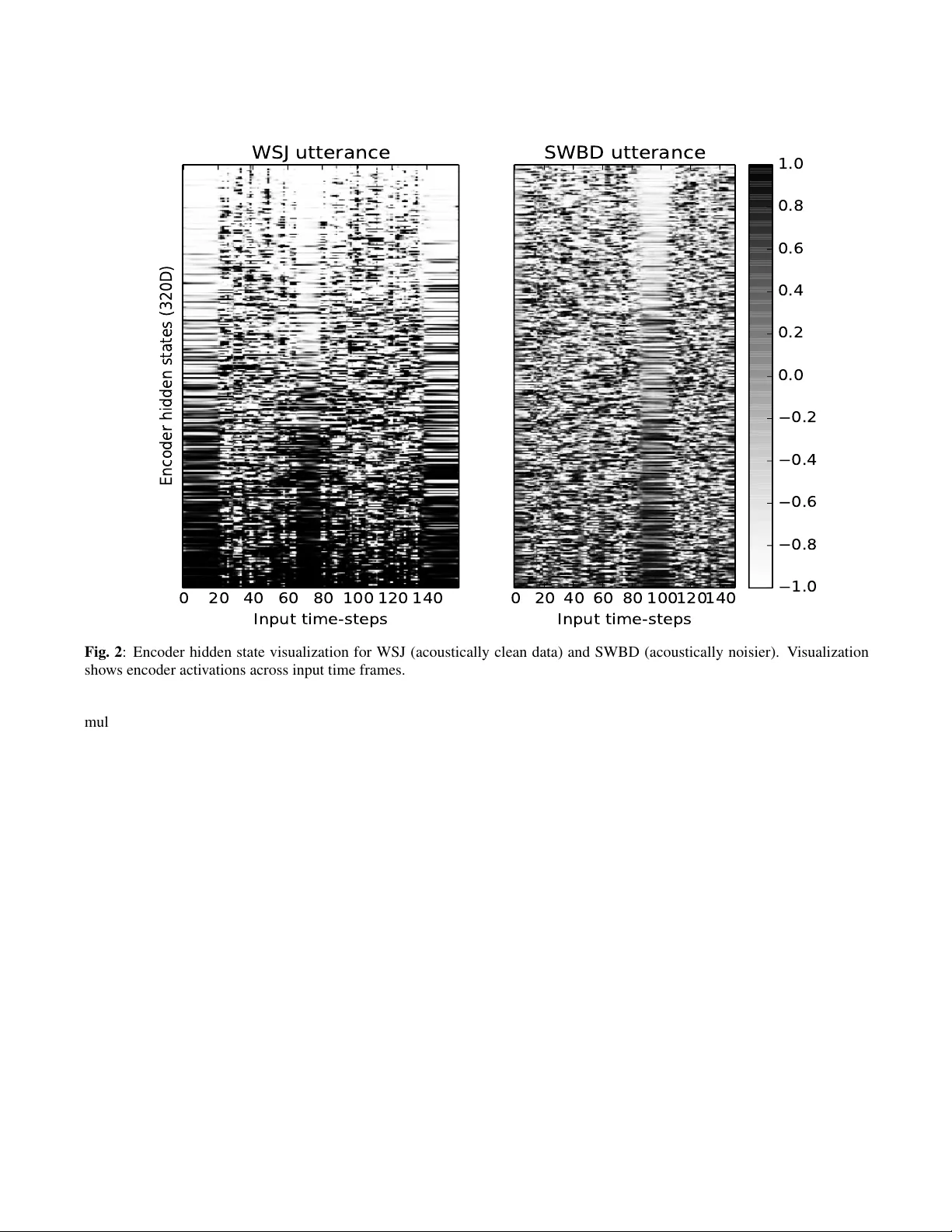
A COUSTIC-TO-W ORD RECOGNITION WITH SEQUENCE-T O-SEQUENCE MODELS Shruti P alaskar and Florian Metze Carnegie Mellon Uni versity Language T echnologies Institute Pittsbur gh, P A, USA { spalaska | fmetze } @cs.cmu.edu ABSTRA CT Acoustic-to-W ord recognition provides a straightforward solution to end-to-end speech recognition without needing ex- ternal decoding, language model re-scoring or lexicon. While character-based models of fer a natural solution to the out-of- vocab ulary problem, word models can be simpler to decode and may also be able to directly recognize semantically mean- ingful units. W e present effecti ve methods to train Sequence- to-Sequence models for direct word-le vel recognition (and character-le vel recognition) and show an absolute improv e- ment of 4.4-5.0% in W ord Error Rate on the Switchboard corpus compared to prior work. In addition to these promis- ing results, word-based models are more interpretable than character models, which hav e to be composed into words us- ing a separate decoding step. W e analyze the encoder hid- den states and the attention behavior , and sho w that location- aware attention naturally represents words as a single speech- word-vector , despite spanning multiple frames in the input. W e finally sho w that the Acoustic-to-W ord model also learns to segment speech into words with a mean standard de via- tion of 3 frames as compared with human annotated forced- alignments for the Switchboard corpus. Index T erms — end-to-end speech recognition, encoder - decoder , acoustic-to-word, speech embeddings 1. INTR ODUCTION Direct Acoustic-to-W ord (A2W) mapping is rele vant for Au- tomatic Speech Recognition (ASR) because it no longer re- quires a le xicon or separately-trained language model, that is currently necessary to decode in a grapheme, phoneme, char- acter or sub-word models. It would lead to truly end-to-end speech recognition models giving P(W ords | Acoustics). An- other strong motiv ation for b uilding direct word models is to obtain semantically meaningful representations that would be useful in co-learning tasks with other modalities like text where the unit of representation is generally words. Recently , A2W models hav e been explored in order to hav e a simpler and efficient solution for end-to-end recogni- tion. The challenges of these models are how to handle the large word vocab ularies without requiring thousands of hours of data. As a way to manage that problem, [1] restricts the vocab ulary to 10,000 frequently occurring words or resorts to using sub-word units to av oid out-of-vocab ulary (OO V) words. But both of these approaches have certain drawbacks. First, restricted vocab ulary leads to OO V words. And in ad- dition to that, sub-w ord units are not semantically or syntac- tically as rich as whole-w ord units. In this paper, we present a large vocabulary full word model that does not have these constraints. For end-to-end speech recognition, Recurrent Neural Net- work (RNN) acoustic models paired with Connectionist T em- poral Classification (CTC) [2, 3] or attention-based Sequence- to-Sequence (S2S) models [4, 5, 6, 7] pro vide a more po wer - ful and simple framew ork that scales well with large training corpora. These sequence-based models no longer need pre- defined alignments between acoustic features and transcrip- tions, and this flexibility makes working to wards A2W mod- els a possibility now . Recently , notable progress has been made to wards b uild- ing direct A2W models using CTC [8, 9, 10, 11] but it either requires large training data [9, 10, 12] or smaller v ocabulary [1, 8, 11]. In this paper , we present one such approach using no more than 300 hours of training data but with a S2S model instead of a CTC model. Our moti v ation for using a S2S model is that while CTC follows a monotonic alignment between acoustic frames and word predictions, an A2W model would benefit more from a flexible alignment scheme between acoustics and words. As spoken words are more variable in a number of frames per word as compared to the number of frames for characters or phonemes, enforcing a monotonicity for such alignment would be an overhead. Especially in spontaneous speech, or noisy , or multi-speaker scenarios, the labels may not be 100% accurate and model will benefit with flexibility . W ith this method, we can use direct acoustic-to-word modeling in other sequence-based tasks like part-of-speech tagging or syntactic parsing with speech input. An A2W model may sho w better interpretability as it di- rectly maps two correlated streams of data, end-to-end i.e. speech to words. In this paper , we explore the interpretabil- ity , in particular, we analyze the encoder hidden states and the attention mechanism of a S2S model. In the process, we find that this model learns to segment input speech into words, si- lence, and non-silence parts without any added supervision for this segmentation. W e also find that the word-alignments produced by our model are as accurate as human annotated segmentations. Using this learned segmentation, we are able to directly obtain speech-word-vectors from these models. 2. RELA TED WORK A2W modeling has been largely pursued using CTC models. Soltau et al. [10] introduced the first A2W model but needed a very large training corpus (125,000 hours) due to the lar ge vo- cabulary of A2W models, 100000 words in their case. These word v ocabularies are noticeably much lar ger than character or sub-word vocab ularies. Audhkhasi et al. [8] found that fil- tering out rare words and replacing them with an OOV symbol alleviates the need for large data. But producing OO V would lead to higher word error rates. A common technique to solve this OO V problem has been to use word-lev el prediction for frequent words and revert to the character or sub-word predic- tion for rare w ords [9, 1]. This is a tw o-step procedure, stray- ing from the regular sequence-to-sequence mapping of acous- tics to units. Recently , Li et al. [9] proposed a hybrid-CTC model where an A2W model consulted an Acoustic-to-Letter model upon generation of the OO V symbol. They also pro- posed a mixed-unit CTC model using frequent words, letters and sub-words although again with large amounts of data (ap- proximately 3,400 hours). In [1], the authors propose a Spell and Recognize model where they first predict the “spelling” of the w ord before composing it into a word unit (if a frequent word), or preserving the “spelling” as character units. This approach is single-step method as they use a common soft- max for the mixed v ocabularies. All these methods described abov e use the CTC loss function. S2S models have also been used for recognizing sub-word [13] or word-piece units in ASR [14, 12, 7] that no longer hav e OO V w ords but these results were presented with 12,500 hours of in-house speech data. Lu et al. [15] present one of the first S2S models for lar ge vocab ulary A2W recognition with the 300 hour Switchboard corpus with a vocab ulary of 30,000 words. In this paper , we build upon their methods and present an effecti ve w ay of training end-to-end A2W models with improv ed performance. Another area of research that our paper is relev ant to is speech-vector representation learning. [16, 17, 18, 19] all ex- plore ways to extract speech embeddings. Their methods are commonly unsupervised learning based on clustering where they do not use the transcripts or do not perform speech recog- nition. In this work, we obtain similar speech-vectors as a by-product of our speech recognition. 3. SEQUENCE-T O-SEQUENCE MODEL Our S2S model is similar in structure to the Listen, At- tend and Spell model [20] which consists of 3 components: the encoder network, a decoder network and an attention model. The encoder maps the input acoustic features vec- tors x = ( x 1 , x 2 , ..., x T ) where x i ∈ R d into a sequence of higher-le vel features h = ( h 1 , h 2 , ..., h T 0 ) . The encoder is a multi-layer bi-directional Long Short T erm Memory (BLSTM) RNN that is structured as a pyramid by skipping ev ery other frame between certain encoder layers for ef ficient training. This reduces the length of the input from T to T 0 . This encoder network is analogous to the traditional acoustic model of an ASR. The decoder network is also an LSTM network that learns to model the output distrib ution ov er the next target conditioned on sequence of previous predictions i.e. P ( y l | y ∗ l − 1 , y ∗ l − 2 , ..., y ∗ 0 , x ) where y ∗ = ( y ∗ 0 , y ∗ 1 , ..., y ∗ L +1 ) is the ground-truth label sequence. In this work, y ∗ i ∈ U can be a token from a character , sub-word or word vocabulary . This decoder network is similar to the language model in traditional ASR as it generates targets y from h using an at- tention mechanism. The attention model learns an alignment weight vector between the encoding h and the current output of decoder y l . At each time step, the attention module com- putes a context vector that is fed into the decoder together with the previous ground-truth label y ∗ l − 1 . W e use a location-aw are attention mechanism [21] that enforces monotonicity in the alignments, which may be ben- eficial for speech recognition. T o do so, the location-aware attention applies a con volution across time to the attention of previous time step using trainable filters. This con volved attention feature is used for calculating the attention for the current time step. W e apply a one-dimensional conv olution K along the input feature axis t to get a set of T features { f } T t =1 described as follows: { f } T t =1 = K ∗ a l − 1 e lt = g T tanh (Lin ( y l − 1 ) + Lin ( h ) + LinB ( f t )) a lt = Softmax ( { e lt } T t =1 ) where a l − 1 = [ a l − 1 , 1 , ..., a l − 1 ,T ] T , g is a learnable vector pa- rameter , { e lt } T t =1 is a T -dimensional vector , Lin() is a linear layer with learnable matrix parameters without bias vectors, LinB() is a linear layer with learnable matrix and bias param- eters. The S2S model is trained by optimizing the cross entrop y loss function which maximizes the log-likelihood of the train- ing data. W e use beam search to perform inference. W e also apply unigram label smoothing that distributes the probability of most-probable token to prev ent the over -confidence of the model [22, 23]. 4. EXPERIMENT AL SETUP W e use the standard 300-hour Switchboard corpus (SW , LDC97S62) [24] which consists of 2,430 two-sided tele- phonic con versations between 500 different speakers and contains 3 million words of text. W e ev aluate on the HUB5 ev al2000 (LDC2002S09, LDC2002T43) containing Switch- board subset similar to training data and CallHome (CH) subset that is a tougher set. There are 196,656 total utterances out of which we use the first 4,000 utterances as a valida- tion set. Our input features are 80-dimensional log-mel filter banks normalized with per-speak er mean and v ariance. W e also use 3-dimensional pitch features. W e present three dif ferent types of target units for speech recognition in this paper: characters, BPE units and words. The character vocab ulary is made of 46 units containing 26 letters, 10 digits, and other frequently occurring special sym- bols. W e try dif ferent BPE vocab ularies like 300, 500, 1k, 5k, 10k and 16k. W e finally present a large-v ocabulary model made of all 29,874 unique words in the Switchboard set. The vocab ularies also contain non-language special symbols that denote noise, v ocalized-noise and laughter . W e train charac- ter and word le vel RNN language models on the Switchboard + Fisher (LDC2004T19) [25] transcripts as is the common practice for this data. Our encoder consists of 6 layers each with 320 bi- directional LSTM cells. The second and third layer skip ev ery other frame to get a reduction of T / 4 in input frames. W e use the AdaDelta [26] optimizer . The location-aware attention con volution uses 10 filters with width 100. W e use a projection layer of 320 dimensions after each layer of the encoder . Our decoder is a single layer LSTM contain- ing 300 cells. W e initialize all parameters uniformly within [ − 0 . 1 , 0 . 1] unless otherwise specified. W e use unigram la- bel smoothing with weight 0.05. The beam size used for all experiments is 10. W e use the ESPnet toolkit[27, 28] as a starting point for our experiments. 5. RESUL TS In T able 1, we present our character-le vel S2S model and compare with pre viously published CTC and S2S models, us- ing the 300h SW corpus and character v ocabularies for better understanding. According to these results, our models obtain the best W ord Error Rate (WER) in both SW and CH test sets among the S2S models with and without a language model. W e also perform better than all CTC models in the SW test set and the difference in the CH set is minor . Furthermore, we observe a 13% relativ e improvement in the SW subset by using an RNNLM with shallow fusion [29] which is trained at the character and word le vel. In T able 2, we present the A2W models with BPE and word units. Our first model consists of words occurring at least 5 times (W ord > = 5) in the training set that led to 11069 T able 1 : W ord Error Rate (WER) for the SW and CH test sets using character target units , and comparison with other end-to-end character-le vel models. W e compare with the re- scored character-LM results from prior w ork when av ailable. WER (%) Model V ocab SW CH Prior W ork CTC Hannun et al. +LM [30] 29 20.0 31.8 Zweig et al. +LM [31] 79 19.8 32.1 Audhkhasi et al. [1] 79 18.9 30.9 Prior W ork S2S Lu et al. +LM [15] 35 32.6 51.9 Zenkel et al. [32] 46 28.1 40.6 T oshniwal et al. [33] N/A 23.1 40.8 Our models S2S Char 46 18.0 32.5 S2S Char +LM 46 17.1 31.1 S2S Char +W ord LM 46 15.6 31.0 T able 2 : W ord Error Rate (WER) for the SW and CH test sets using BPE and word level target units , and comparison with other end-to-end w ord-lev el models. * denotes character initialization WER (%) Model V ocab SW CH Prior W ork CTC Audhkhasi et al. [1] 10000 14.5 23.9 Chen et al. [34] 29874 24.9 36.5 Prior W ork S2S Chen et al. [34] 29874 31.2 40.5 Lu et al. [15] 29874 26.8 48.2 Lu et al. +LM [15] 29874 26.2 47.4 Our models S2S BPE 12k 11690 21.3 35.7 S2S W ord > = 5 11069 23.0 37.2 S2S W ord > = 5* 11069 22.4 36.1 S2S Large V ocab 29874 22.4 36.2 S2S Large V ocab + LM 29874 22.1 36.3 words but with an OO V rate of 2.3% in the e v al2000 test set. T o address this high OO V rate, we tried to match the w ord vo- cabulary by an equi valent BPE vocab ulary of 12k merge op- erations. This model performed better than the word model as expected. W e also e xperiment with initializing the word > = 5 model with a pretrained character model (similar to [1]) for better con ver gence and observe impro vements. Our second model is a large vocab ulary model made of all the words in the training set. This model performs better than the previous word model which may be due to absence of the frequently occurring OO V token. W e get an absolute im- prov ement of 4.4% and 12% in SW and CH subsets o ver our baseline [15] without a language model. Ideally , S2S A2W model does not need a separate language model as it directly predicts a sequence of w ords using the decoder LSTM. But as the LM is trained on a larger corpus, we integrate it to check its ef fect and do not observe improvements as large as the character model. Comparison with CTC. The v ocabularies of CTC mod- els (both character and word) is different than ours hence models are not comparable. Prior work in CTC [1] has almost 20,000 less words than our model and they used strong hyper parameter tuning techniques to arriv e at a successful A2W model. On a similar setup, their character-based model is worse by 5% WER. In the paper , the y do not pro vide a reason for this behavior . In our S2S model, we observe the reverse trend i.e. the word-model performs worse than character- model. This is an interesting trend for CTC and S2S mod- els and needs further exploration. W e note that CTC and S2S models are not comparable with each other due to critical dif- ferences in loss computation. 6. A TTENTION ANAL YSIS In the follo wing two sections we analyze the beha vior of S2S models, specifically for the A2W recognition task. W e ana- lyze attention in the decoder and the hidden representations of the encoder . Human Annotated W ord Boundaries in SWBD. NXT Switchboard Annotations (LDC2009T26) are a subset of the Switchboard corpus (LDC97S62) containing 1 million w ords that were annotated for syntactic structure and disfluencies as part of the Penn Treebank project. This subset of the Switchboard corpus contains human annotated word-le vel forced alignments that mark the beginning and end of each word in the utterance in time 1 . In the follo wing sections, we analyze attention behavior of the A2W model and the speech-word-vectors obtained from it. T o do this analysis, we need groundtruth word-lev el segmentations and this corpus is a good match. From NXT Switchboard, we choose those utterances that are also present in the T reebank-3 (LDC99T42) corpus. The speech in this corpus is re-segmented to match the sentences in T reebank-3. W e filter out utterances with less than 3 words resulting in 67,654 utterances in total. This is di vided into 56,100 train, 5,829 validation and 5,725 test sets. W e train a separate A2W model with this data in the same setup as de- scribed in Section 4, without using any explicit information about word-se gments. W e only train on this dataset to avoid introducing a more v ariability in our analysis, i.e. are the seg- mentations due to our model or due to training with a larger corpus (SW 300h)? In our setup, we split compound words into two words (e g. they‘re − → they and ‘re). 1 http://groups.inf.ed.ac.uk/switchboard/ structure.html 0 20 40 60 80 100 120 140 160 Input time-steps 0.0 0.1 0.2 0.3 0.4 0.5 0.6 0.7 0.8 Attention Probabilities maybe they 're just too involved for the person to go and sit through them you know Fig. 1 : Attention visualization for a sample utterance from the v alidation set shows highly localized attention for a word- lev el S2S model 6.1. Attention Beha vior In Figure 1 we plot the attention of a sample utterance from our v alidation set of the corpus. W e notice that the attention is very peaky and focuses only on certain frames in the input although generally a word spans multiple input frames. T o understand this beha vior of the model, let us re visit the location-aware attention explained in Section 3. The location- aware attention is useful in speech to enforce a monotonic alignment between source and target. It does so by con volv- ing the pre vious attention vector along input time-steps and feeding it as another input parameter while calculating atten- tion of the current time step. This way , the model is informed where to pay attention “next” and would mostly look in the “future” to make a prediction. As this model is trained to wards word-units and the atten- tion is focused only on certain frames, we speculate that the hidden states corresponding to those frames are the speech- word-vectors for those words. Here, we are able to extract speech-word-vectors from an end-to-end model trained for direct word recognition without the need of any predefined forced-alignments. The size of these embeddings is equal to the number of RNN cells in the last layer of the encoder . 6.2. A utomatic Segmentation of Speech into W ords Giv en that the attention is highly localized, we attempt to quantify whether the attention weights corresponded to ac- tual word boundaries. From the Switchboard NXT dataset, we chose all utterances (train, validation and test) for which we hav e 0% WER during testing. 39% of the total utterances hav e 0 WER. W e perform decoding with beam size 1 here. W e conv erted the human-annotated forced-alignments to their corresponding frame numbers using the 10ms frame rate of our model. The predicted frame number is calculated from the attention distribution shown in Figure 1 as follows. The input frame with the max attention probability is chosen as the predicted frame for the word. The frame error is calculated at each word lev el by taking an absolute difference between the predicted and grouthtruth frame number . A positi ve dif- ference means the predicted frame was after the groundtruth alignment, and a negati ve difference means that it was be- fore. W e av erage this frame error for all words in all utter- ances (171073 words). An example of this computation is Predicted = [988 , 1008 , 1012 , 1044 , 1092] Groundtruth = [988 , 1005 , 1013 , 1042 , 1100] and Frame Error = [0 , +3 , − 1 , +2 , − 8] . The attention weights for the last word predicted in the sequence is often most erroneous. As an example, in Fig- ure 1 we see that “know”, the last word, has a distributed attention weight, and has the least probability value (approx- imately 0.2) compared to other words. For better understand- ing, we also compute frame errors without considering the last word of e very utterance. W e compute the mean and standard deviation of frame errors for all words. During training, we use a pyramidal encoder that reduces the input frame lengths by a factor of 4. Hence, while computing mean and standard deviation of frame errors, we scale them by 4 as well for fair comparison. The standard deviation of frame error without including last word is 3.6 frames after the groundtruth. For a word-based model, this is an encouraging result as usually a character unit spans 7 (or 1.75 frames after a pyramidal encoder) and a word would span many more. T able 3 : A verage frame error mean and standard deviation (std de v .) between groundtruth forced-alignments and S2S word segment prediction A vg. Frame Error T rain V al T est W/o Last W ord - Mean 0 -0.08 -0.01 W/o Last W ord - Std Dev 3.7 3.3 2.0 All W ords - Mean 0.4 0.3 0.3 All W ords - Std Dev 10.1 9.8 10.5 Why does attention f ocus on the end of word? The op- timization task in A2W recognition is to map a sequence of input frames (usually larger number of input frames than in character or BPE prediction models) to a sequence of target words. During training, the model learns where word bound- aries occur by recognizing the attention distrib ution that leads to highest probability of generating the correct output. The bi-directional LSTM in the encoder has access to the past as well as future input. Therefore, the encoder learns to look into the future to recognize where a different word is beginning, and the BLSTM would hold richest embeddings in the unit corresponding to each of frame of the current word. W e in- vestigate the encoder embeddings in the next section in more detail. It is also important to note that the location-aware at- tention constrains the model to only look into the future, and not the past, which would push the boundaries towards word ends rather than beginnings. Hence, the attention mechanism learns to focus mostly on the word boundaries. W e obtain a context vector from the attention mechanism that is a weighted sum of the encoder hidden states. Follo wing this peaky nature of the attention mechanism, we expect to see certain patterns reflected in the encoder embeddings. This is explored in the follo wing section. 7. SPEECH EMBEDDINGS W e train a similar A2W model on the W all Street Journal cor - pus (WSJ, LDC93S6B and LDC94S13B) which comprises about 90 hours of read speech in clean acoustic en viron- ments with a close-talk microphone. This dataset has about 300 different speakers in the train, validation (de v93) and test (ev al92) sets. WSJ is sampled at 16kHz while SWBD is sampled at 8kHz and we upsample SWBD to 16kHz for implementation reasons. W e bring the readers attention to these major differences in acoustic and speaker variability and domain of the data in WSJ and SWBD. In Figure 2 we visualize the encoder hidden states for sample utterances from the validation sets of WSJ (4k8c030h) and SWBD (same as in Figure 1). W e train a WSJ model to compare hidden state activ ations of the noisier SWBD dataset with a clean WSJ dataset as we e xpect the acti vation patterns to be clearer and more interpretable in the cleaner dataset. The hidden state dimension here is same as the number of BLSTM cells in the last encoder layer (320D). For this visualization, we sort the hidden states of the encoder in an ascending order of total activ ation over time. W e use a tanh non-linearity hence all values range from -1 to +1. W e note that there are three types of patterns to observe in these acti v ations: 1) stable horizon- tal lines, 2) disruptions, and 3) vertical dashed-line pattern across encoder hidden states (Y -axis) within the disruptions. Pattern 3 is easier to notice in the WSJ acti v ations. Upon listening to these utterances, we found that sta- ble horizontal lines (pattern 1) corresponds to silence in the utterance, while disruptions (pattern 2) corresponds to the speech. W e observe similar patterns identifying speech and non-speech in both WSJ and SWBD. From this, we under- stand that the model has learned to detect and segment pauses in speech. As WSJ is the acoustically cleaner corpus with less variability , “silence” acoustics are stable and repetitiv e throughout, which is what we observ e in the be ginning, mid- dle and end of the WSJ utterance–while the SWBD “silence” activ ations look different. In WSJ, we can further identify 0 20 40 60 80 100 120 140 Input time-steps Encoder hidden states (320D) WSJ utterance 0 20 40 60 80 100 120 140 Input time-steps SWBD utterance 1.0 0.8 0.6 0.4 0.2 0.0 0.2 0.4 0.6 0.8 1.0 Fig. 2 : Encoder hidden state visualization for WSJ (acoustically clean data) and SWBD (acoustically noisier). V isualization shows encoder acti vations across input time frames. multiple vertical dashed-line patterns across all encoder hid- den states (i.e. Y -axis; pattern 3). This pattern is formed by encoder units turning on and of f (+1, -1) when a word bound- ary is reached. This particular WSJ utterance has 15 words and we observe 15 vertical dashed-line patterns in the acti- vations. This further reinstates that we are able to represent multiple frames of speech using single 320D speech-word- vectors. Pattern 3 is tougher to spot in SWBD comparativ ely but still noticeable; it might need more training data or better regularization with this data to obtain similar properties as the WSJ model. 8. CONCLUSION In this paper , we presented promising results on character- based and word-based S2S models on the 300 hour Switch- board corpus with improved training strategies. W e then show a quantitative analysis of model beha vior by analyzing the en- coder hidden states and attention mechanism. W e find that the model learns to segment speech into word, silence, and non-silence parts without any supervision other than word- lev el transcripts (with utterance lev el alignments). W e also show that it is possible to extract speech-word-vectors from this type of model. As a follo w up study , we would like to explore this behavior on corpora other than Switchboard or W all Street Journal. 9. A CKNO WLEDGEMENTS W e thank Desmond Elliot, Amanda Duarte, Ozan Caglayan and Jindrich Libovick y for their valuable feedback on this writeup. W e also thank the CMU speech group for many use- ful discussions. W e gratefully acknowledge the support of NVIDIA Corporation with the donation of the T itan X Pascal GPUs used for this research. This work is partially supported by the D ARP A AID A grant. A ppendix In this section, we in vestigate the Speech Embeddings fur- ther using TSNE visualization and finding nearest neighbors of each acoustic-word-embedding. In Figure 3 and T able 4 we see “same” words cluster together . 15 10 5 0 5 10 15 10 5 0 5 10 15 20 now i 'm uh uh oh i well that that that would be true so it 's been a real interesting thing for them and uh i think that was a big for them to all their ways of changing things too my i have my year old mother living with us do you like it i do n't know it 's not up oh i see that 's really neat and so we did you know we did try when they were very young i did not work so it was a it was a you know but there were always things that just out and they went off oh and you 're kidding i really do n't it must be we got a pretty fair amount of snow well like i said good luck to you and and it 's not it 's not just that i think so too and it 's sad i think it 's real important to play sports i think Fig. 3 : TSNE visualization of 300 randomly selected speech embeddings. W e observe that same words occur close together which shows that the embeddings are good representations of the w ords. 10. REFERENCES [1] Kartik Audhkhasi, Brian Kingsbury , Bhuvana Ramab- hadran, George Saon, and Michael Picheny , “Build- ing competitiv e direct acoustics-to-w ord models for en- glish con versational speech recognition, ” arXiv pr eprint arXiv:1712.03133 , 2017. [2] Alex Gra ves, Santiago Fern ´ andez, F austino Gomez, and J ¨ urgen Schmidhuber , “Connectionist temporal classifi- cation: labelling unsegmented sequence data with recur- rent neural networks, ” in Pr oc. ICML , 2006, pp. 369– 376. [3] Alex Grav es and Navdeep Jaitly , “T owards end-to-end speech recognition with recurrent neural networks, ” in Pr oc. ICML , 2014. T able 4 : Nearest Neighbor search ov er acoustic-word-embeddings. T able shows 10 nearest neighbor for a particular word. W ords shown belo w are randomly chosen. word nearest neighbors oh oh, oh, oh, oh, oh, oh, oh, oh, #eos#, oh i i, i, i, i, i, i, i, i, i, i see see, see, see, see, see, see, see, see, see, see #eos# #eos#, #eos#, #eos#, #eos#, #eos#, #eos#, #eos#, #eos#, #eos#, #eos# that that, that, that, that, that, that, neat, obviously , that, it ’ s ’ s, ’ s, #eos#, ’ s, ’ s, ’ s, you, ’ s, ’ s, ’ s really really , know , a, so, really , really , really , really , well, really neat neat, me, neat, #eos#, neat, neat, neat, neat, #eos#, funny #eos# #eos#, #eos#, #eos#, #eos#, #eos#, well, #eos#, she, #eos#, #eos# and and, and, i, and, and, #eos#, and, and, and, and so so, so, so, so, so, couple, know , so, well, so we we, they , we, we, #eos#, we, we, go, we, they did did, just, just, tell, just, just, in, just, because, goes you you, you, east, of, you, you, you, you, thing, you know know , know , know , know , know , know , know , know , would, know [4] Ilya Sutskev er , Oriol V inyals, and Quoc V Le, “Se- quence to sequence learning with neural networks, ” in Pr oc. NIPS , 2014. [5] Jan Choro wski, Dzmitry Bahdanau, Kyunghyun Cho, and Y oshua Bengio, “End-to-end continuous speech recognition using attention-based recurrent NN: First re- sults, ” arXiv preprint , 2014. [6] Ashish V aswani, Noam Shazeer , Niki Parmar , Jakob Uszkoreit, Llion Jones, Aidan N Gomez, Lukasz Kaiser , and Illia Polosukhin, “ Attention is all you need, ” in Ad- vances in Neural Information Pr ocessing Systems , 2017, pp. 6000–6010. [7] Kanishka Rao, Has ¸ im Sak, and Rohit Prabhav alkar , “Exploring architectures, data and units for stream- ing end-to-end speech recognition with rnn-tra nsducer , ” in Automatic Speech Recognition and Understanding W orkshop (ASRU), 2017 IEEE . IEEE, 2017, pp. 193– 199. [8] Kartik Audhkhasi, Bhuv ana Ramabhadran, George Saon, Michael Picheny , and David Nahamoo, “Direct acoustics-to-word models for english conv ersational speech recognition, ” arXiv pr eprint arXiv:1703.07754 , 2017. [9] Jinyu Li, Guoli Y e, Amit Das, Rui Zhao, and Y ifan Gong, “ Advancing acoustic-to-word ctc model, ” arXiv pr eprint arXiv:1803.05566 , 2018. [10] Hagen Soltau, Hank Liao, and Hasim Sak, “Neural speech recognizer: Acoustic-to-w ord lstm model for large v ocabulary speech recognition, ” arXiv preprint arXiv:1610.09975 , 2016. [11] Thomas Zenkel, Ramon Sanabria, Florian Metze, and Alex W aibel, “Subword and crossword units for ctc acoustic models, ” arXiv preprint , 2017. [12] Chung-Cheng Chiu, T ara N Sainath, Y onghui W u, Rohit Prabhav alkar , Patrick Nguyen, Zhifeng Chen, Anjuli Kannan, Ron J W eiss, Kanishka Rao, Katya Gonina, et al., “State-of-the-art speech recognition with sequence-to-sequence models, ” arXiv pr eprint arXiv:1712.01769 , 2017. [13] Rico Sennrich, Barry Haddow , and Alexandra Birch, “Neural machine translation of rare words with subword units, ” arXiv preprint , 2015. [14] W illiam Chan, Y u Zhang, Quoc Le, and Na vdeep Jaitly , “Latent sequence decompositions, ” arXiv pr eprint arXiv:1610.03035 , 2016. [15] Liang Lu, Xingxing Zhang, and Steve Renals, “On training the recurrent neural network encoder -decoder for large vocab ulary end-to-end speech recognition, ” in Acoustics, Speech and Signal Pr ocessing (ICASSP), 2016 IEEE International Confer ence on . IEEE, 2016, pp. 5060–5064. [16] Y u-An Chung and James Glass, “Speech2v ec: A sequence-to-sequence framework for learning word embeddings from speech, ” arXiv preprint arXiv:1803.08976 , 2018. [17] Herman Kamper , W eiran W ang, and Karen Livescu, “Deep con volutional acoustic word embeddings using word-pair side information, ” in Acoustics, Speech and Signal Processing (ICASSP), 2016 IEEE International Confer ence on . IEEE, 2016, pp. 4950–4954. [18] David Harwath and James Glass, “Deep multimodal semantic embeddings for speech and images, ” arXiv pr eprint arXiv:1511.03690 , 2015. [19] Samy Bengio and Georg Heigold, “W ord embeddings for speech recognition, ” in F ifteenth Annual Confer- ence of the International Speec h Communication Asso- ciation , 2014. [20] W illiam Chan, Navdeep Jaitly , Quoc Le, and Oriol V inyals, “Listen, attend and spell: A neural network for large vocabulary conv ersational speech recognition, ” in Acoustics, Speech and Signal Pr ocessing (ICASSP), 2016 IEEE International Confer ence on . IEEE, 2016, pp. 4960–4964. [21] Jan K Chorowski, Dzmitry Bahdanau, Dmitriy Serdyuk, Kyungh yun Cho, and Y oshua Bengio, “ Attention-based models for speech recognition, ” in Advances in neural information pr ocessing systems , 2015, pp. 577–585. [22] Gabriel Pereyra, George T ucker , Jan Chorowski, Lukasz Kaiser , and Geof frey Hinton, “Regularizing neural networks by penalizing confident output distributions, ” arXiv pr eprint arXiv:1701.06548 , 2017. [23] Jan Chorowski and Navdeep Jaitly , “T owards better de- coding and language model integration in sequence to sequence models, ” arXiv pr eprint arXiv:1612.02695 , 2016. [24] John J Godfrey , Edward C Holliman, and Jane Mc- Daniel, “Switchboard: T elephone speech corpus for research and dev elopment, ” in Acoustics, Speech, and Signal Pr ocessing, 1992. ICASSP-92., 1992 IEEE Inter- national Confer ence on . IEEE, 1992, vol. 1, pp. 517– 520. [25] Christopher Cieri, David Miller, and Ke vin W alker , “The fisher corpus: a resource for the next generations of speech-to-text., ” in LREC , 2004, vol. 4, pp. 69–71. [26] Matthew D Zeiler , “ Adadelta: an adapti ve learning rate method, ” arXiv preprint , 2012. [27] Suyoun Kim, T akaaki Hori, and Shinji W atanabe, “Joint ctc-attention based end-to-end speech recognition using multi-task learning, ” in Acoustics, Speech and Signal Pr ocessing (ICASSP), 2017 IEEE International Confer- ence on . IEEE, 2017, pp. 4835–4839. [28] Shinji W atanabe, T akaaki Hori, Suyoun Kim, John R Hershey , and T omoki Hayashi, “Hybrid ctc/attention architecture for end-to-end speech recognition, ” IEEE Journal of Selected T opics in Signal Pr ocessing , vol. 11, no. 8, pp. 1240–1253, 2017. [29] Caglar Gulcehre, Orhan Firat, Kelvin Xu, K yunghyun Cho, Loic Barrault, Huei-Chi Lin, Fethi Bougares, Hol- ger Schwenk, and Y oshua Bengio, “On using mono- lingual corpora in neural machine translation, ” arXiv pr eprint arXiv:1503.03535 , 2015. [30] A wni Hannun, Carl Case, Jared Casper, Bryan Catan- zaro, Greg Diamos, Erich Elsen, Ryan Prenger , San- jeev Satheesh, Shubho Sengupta, Adam Coates, et al., “Deep speech: Scaling up end-to-end speech recogni- tion, ” arXiv preprint , 2014. [31] Geoffre y Zweig, Chengzhu Y u, Jasha Droppo, and An- dreas Stolcke, “ Adv ances in all-neural speech recog- nition, ” in Acoustics, Speech and Signal Pr ocess- ing (ICASSP), 2017 IEEE International Conference on . IEEE, 2017, pp. 4805–4809. [32] Thomas Zenkel, Ramon Sanabria, Florian Metze, Jan Niehues, Matthias Sperber, Sebastian St ¨ uker , and Alex W aibel, “Comparison of decoding strategies for ctc acoustic models, ” arXiv preprint , 2017. [33] Shubham T oshniwal, Hao T ang, Liang Lu, and Karen Liv escu, “Multitask learning with lo w-le vel auxiliary tasks for encoder-decoder based speech recognition, ” arXiv pr eprint arXiv:1704.01631 , 2017. [34] Zhehuai Chen, Qi Liu, Hao Li, and Kai Y u, “On modu- lar training of neural acoustics-to-word model for lvcsr , ” arXiv pr eprint arXiv:1803.01090 , 2018.