Subspace-Orbit Randomized Decomposition for Low-rank Matrix Approximation

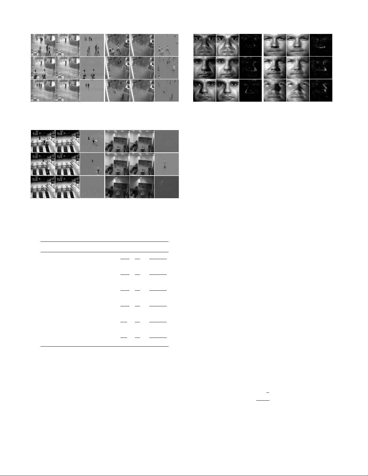
1 Subspace-Orbit Randomized Decomposition for Lo w-rank Matrix Approximation Maboud F . Kaloorazi † , and Rodrigo C. de Lamare † , ‡ † Centre for T elecommunications Studies (CETUC) Pontifical Catholic Uni versity of Rio de Janeiro, Brazil ‡ Department of Electronics, Uni versity of Y ork, United Kingdom E-mail: { kaloorazi,delamare } @cetuc.puc-rio.br Abstract —An efficient, accurate and reliable approximation of a matrix by one of lower rank is a fundamental task in numerical linear algebra and signal processing applications. In this paper , we introduce a new matrix decomposition appr oach termed Subspace-Orbit Randomized singular value decomposition (SOR- SVD), which makes use of random sampling techniques to give an appr oximation to a low-rank matrix. Given a large and dense data matrix of size m × n with numerical rank k , where k  min { m, n } , the algorithm requir es a few passes through data, and can be computed in O ( mnk ) floating-point opera- tions. Moreov er , the SOR-SVD algorithm can utilize advanced computer ar chitectures, and, as a result, it can be optimized for maximum efficiency . The SOR-SVD algorithm is simple, accurate, and pro vably correct, and outperforms pre viously reported techniques in terms of accuracy and efficiency . Our numerical experiments support these claims. Index T erms —Matrix computations, dimension reduction, low- rank approximation, randomized algorithms. I . I N T R O D U C T I O N C OMPUTING a low-rank approximation of a given data matrix, i.e., approximating the matrix by one of lower rank, is a fundamental task in signal processing and its applications. Such a compact representation of a matrix can provide a significant reduction in memory requirements, and more importantly , computational costs when the computational cost scales according to a high-degree polynomial with the dimensionality . Matrices with low-rank structures arise fre- quently in numerous applications such as latent variable graph- ical modeling, [1], ranking and collaborativ e filtering, [2], background subtraction [3]–[6], system identification [7], IP network anomaly detection [8], [9], subspace clustering [10]– [13], biometrics [14], [15], sensor and multichannel signal pro- cessing [16], statistical process control and multidimensional fault identification [17], [18], DN A microarray data [19], and quantum state tomography [20]. T raditional algorithms for computing a low-rank approxima- tion of a matrix, such as singular value decomposition (SVD) [21] and the rank-re vealing QR decomposition [22], [23] are computationally prohibiti ve for large data sets. Moreov er , standard techniques for their computation are challenging to parallelize in order to take advantage of modern com- puter architectures [24], [25]. Recently de veloped low-rank 1 A primary version of this paper has been submitted to the 26th European Signal Processing Conference (EUSIPCO 2018). approximation algorithms based random sampling techniques, howe ver , hav e been sho wn to be surprisingly efficient, accurate and robust, and are known to outperform the traditional algorithms in many practical situations [26]–[31]. The power of randomized methods lies in the fact they can be optimized for maximum efficienc y on modern architectures. Our Contributions Motiv ated by recent de velopments, this paper proposes a new randomized decompositional approach called subspace- orbit randomized singular value decomposition (SOR-SVD) to compute the lo w-rank approximation of a matrix. Giv en a lar ge and dense rank- k matrix of size m × n , the SOR-SVD requires a fe w passes over the data, and can be computed in O ( mnk ) floating-point operations (flops). The main operations of the algorithm inv olve matrix-matrix multiplication and the QR de- composition. This, due to recently developed Communication- A voiding QR (CA QR) algorithms [32], which are optimal in terms of communication costs, i.e., data movement either between different levels of a memory hierarchy or between processors, allows the algorithm to be optimized for peak machine performance on modern computational platforms. W e provide theoretical error bounds, i.e., lo wer bounds on singular values and upper bounds on the low-rank approxima- tion, for the SOR-SVD algorithm, and experimentally show that the low-rank error bounds provided are empirically sharp for one class of matrices considered. W e also apply the SOR-SVD to solve the RPCA problem [3], [33], [34], i.e., to decompose a data matrix into a low-rank plus a sparse matrix, and study in computer vision applications of background/foreground separation in surveillance video, and shadow and specularity remov al from face images. Notation Bold-face upper-case letters are used to denote matrices. Giv en a matrix A , k A k 1 , k A k 2 , k A k F , k A k ∗ denote the ` 1 -norm, the spectral norm, the Frobenius norm, the nuclear norm, respecti vely . σ j ( A ) denotes the j -th largest singular value of A , and the numerical range of A is denoted by R ( A ) . The symbol E denotes expected value with respect to random variables. Given a random variable Ω , E Ω denotes expectation with respect to the randomness in Ω , and the dagger † denotes the Moore-Penrose pseudo-in verse. W e structure the remainder of this paper as follows. In Section II, we introduce the mathematical model of the data 2 and discuss prior works on randomized algorithms. In Section III, we describe our proposed approach, which also includes a variant that uses the po wer iteration scheme, in detail. Section IV presents our theoretical analysis. In Section V, we present and discuss our numerical experimental results, and our conclusion remarks are giv en in Section VI. I I . M AT H E M A T I C A L M O D E L A N D P R I O R W O R K S Giv en an input matrix A ∈ R m × n , where m ≥ n , with numerical rank k , its singular value decomposition (SVD) [21] is defined as follows: A = U m × n Σ n × n V T n × n =  U k U 0   Σ k 0 0 Σ 0   V k V 0  T , (1) where U k ∈ R m × k , U 0 ∈ R m × n − k hav e orthonormal columns, spanning the range of A and the null space of A T , respectiv ely , Σ k ∈ R k × k and Σ 0 ∈ R n − k × n − k are diagonal containing the singular values, i.e., Σ k = diag ( σ 1 , ..., σ k ) and Σ 0 = diag ( σ k +1 , ..., σ n ) , and V k ∈ R n × k and V 0 ∈ R n × n − k hav e orthonormal columns, spanning the range of A T and the null space of A , respectiv ely . A can be written as A = A k + A 0 , where A k = U k Σ k V T k , and A 0 = U 0 Σ 0 V T 0 . The SVD constructs the optimal rank- k approximation A k to A , as stated in the following theorem. Theor em 1: (Eckart and Y oung [35], and Mirsky [36]) minimize rank ( B ) ≤ k k A − B k 2 = k A − A k k 2 = σ k +1 . (2) minimize rank ( B ) ≤ k k A − B k F = k A − A k k F = v u u t n X j = k +1 σ 2 j . (3) Throughout this paper we focus on the matrix A defined, and m ≥ n > max { k , 2 } . Our results hold for m < n , though. Although, the SVD is numerically stable, accurate and provides detailed information on singular subspaces and sin- gular values, it is expensiv e to compute for large data sets. Furthermore, standard techniques for its computation are chal- lenging to parallelize in order to utilize modern computational platforms [24], [25]. On the other hand, partial SVD based on Krylov subspace methods, such as the Lanczos and Arnoldi algorithms, can construct an approximate SVD of an input matrix, for instance A , best, at a cost O ( mnk ) . Howe ver , the partial SVD suffers from two drawbacks. First, inherently , it is numerically unstable [21], [24], [37]. Second, its methods are challenging to parallelize [30], [31], which makes it unsuitable to apply on modern architectures. Recently dev eloped algorithms based on randomization for low-rank approximations [26]–[31], [38] have attracted considerable attention because i) they are computationally efficient, and ii) they readily lend themselves to a parallel implementation to exploit modern computational architectures. Beginning with [26], many algorithms have been proposed for low-rank matrix approximation. The algorithms in [27], [39], [40], b ulit on Frieze et al. ’ s idea [26], first sample columns of an input matrix with a probability proportional to either their magnitudes or leverage scores, representing the matrix in a compressed form. The submatrix is then used for further computation (post-processing step) using deterministic algorithms such as the SVD and piv oted QR decomposition [21] to obtain the final low-rank approximation. Sarl ´ os [28] proposes a different method based on results of the well- known Johnson-Lindenstrauss (JL) lemma [41]. He showed that random linear combinations of ro ws, i.e., projecting the data matrix onto a structured random subspace, can render a good approximation to a low-rank matrix. The works in [42], [43] hav e further advanced Sarl ´ os’ s idea and construct a low-rank approximation based on subspace embedding. Rokhlin et al. [29] proposes to apply a random Gaussian embedding matrix in order to reduce the dimension of the data matrix. The low-rank approximation is then giv en through computations using the classical techniques on the reduced-sized matrix. In a seminal paper, Halko et al. [30] propose two algorithms based on randomization. (The paper also dev elops modified versions of each for gaining either performance or pass-efficienc y). The first algorithm, randomized SVD , for which the authors provide theoretical analysis and extensi ve numerical experiments, for the matrix A , and integers k ≤ ` < n and q , is described in Alg. 1. Algorithm 1 Randomized SVD (R-SVD) Input: Matrix A ∈ R m × n , integers ` and q , Output: A rank- ` approximation. 1: Draw a random matrix Ω ∈ R n × ` ; 2: Compute Y = ( AA T ) q AΩ ; 3: Compute a QR decomposition Y = QR ; 4: Compute B = Q T A ; 5: Compute an SVD B = e UΣV T ; 6: A ≈ Q e UΣV T . The R-SVD approximates A as follows: i) a compressed matrix Y , through random linear combinations of columns of A is formed, ii) a QR decomposition is performed on Y , where the Q factor constructs an approximate basis for R ( A ) , iii) A is projected onto a subspace spanned by columns of Q , forming B , iv) a full SVD of B is computed. In Alg. 1, q is the number of steps of a power method [29], [30]. Gu [31] applies a slightly modified version of the R-SVD algorithm to improve subspace iteration methods, and presents a new error analysis. The second method proposed in [30, Section 5.5] is a single-pass algorithm, i.e., it requires only one pass through data, to compute a lo w-rank approximation. For the matrix A , the decomposition, which we call two-sided ran- domized SVD (TSR-SVD), is computed as described in Alg. 2. Here B approx is an approximation to B = Q T 1 A Q 2 . The TSR-SVD, howe ver , substantially degrades the quality of the approximation, compared to the R-SVD, e ven for matrices with rapidly decaying singular values. The reason behind is, mainly , poor approximate basis drawn from the row space of A , i.e., Q 2 . Furthermore, for a general input matrix, the authors do not provide theoretical bounds, neither upper bounds on the low-rank approximation nor lo wer bounds on the singular values, for the TSR-SVD algorithm. This work addresses these issues. The work in [5] proposes a rank-rev ealing decomposition method based on randomized sampling techniques; the matrix 3 Algorithm 2 T wo-Sided Randomized SVD (TSR-SVD) Input: Matrix A ∈ R m × n , an integer ` , Output: A rank- ` approximation. 1: Draw random matrices Ψ 1 ∈ R n × ` and Ψ 2 ∈ R m × ` ; 2: Compute Y 1 = AΨ 1 and Y 2 = A T Ψ 2 in a single pass through A ; 3: Compute QR decompositions Y 1 = Q 1 R 1 , Y 2 = Q 2 R 2 ; 4: Compute B approx = Q T 1 Y 1 ( Q T 2 Ψ 1 ) † ; 5: Compute an SVD B approx = e U e Σ e V ; 6: A ≈ ( Q 1 e U ) e Σ ( Q 2 e V ) T . A is compressed, multiplied by orthonormal bases for R ( A ) and R ( A T ) from both sides, columns of the reduced matrix, and accordingly , the bases are permuted, the low-rank approx- imation is giv en by projecting it back to the original space. Independent of the TSR-SVD algorithm [30], this work was dev eloped by drawing inspiration from the randomized rank- rev ealing decomposition algorithm proposed in [5]. Unlike the R-SVD, Alg. 1, [30], [31], which is based on one-sided projection, the SOR-SVD algorithm, similar to the TSR-SVD algorithm, is based on two-sided projection; the data matrix is projected onto a lower -dimensional space using orthonormal bases from both sides, a truncated SVD of the compressed matrix is computed, the approximate SVD is obtained by projecting the data back to the original space. W e also present a variant of the SOR-SVD algorithm, which employs the power method scheme [29], [30] to improve the accuracy of the approximations. Our analysis was inspired by the excellent work of Gu [31]. Ho wev er, unlike the one-sided randomized SVD algo- rithm presented in [31], we perform an analysis of a two- sided randomized algorithm, i.e., the SOR-SVD, and provide theoretical lower bounds on singular values and upper bounds on the low-rank approximation. I I I . S U B S PAC E - O R B I T R A N D O M I Z E D S I N G U L A R V A L U E D E C O M P O S I T I O N In this section, we present a randomized algorithm termed subspace-orbit randomized SVD (SOR-SVD), which com- putes the fixed-rank approximation of a data matrix. W e also present a version of the SOR-SVD with po wer iteration, which improves the performance of the algorithm at an extra computational cost. Giv en the matrix A , and an integer k ≤ ` < n , the basic form of SOR-SVD is computed as follows: using a random number generator , we form a real matrix Ω ∈ R n × ` with entries being independent, identically distributed (i.i.d.) Gaussian random variables of zero mean and unit variance. W e then compute the matrix product: T 1 = AΩ , (4) where T 1 ∈ R m × ` is formed by linear combinations of columns of A by the random Gaussian matrix. T 1 is nothing but a projection onto the subspace spanned by columns of A . Having T 1 , we form the matrix T 2 ∈ R n × ` : T 2 = A T T 1 , (5) where T 2 is constructed by linear combinations of rows of A by T 1 . T 2 is nothing but a projection onto the subspace spanned by ro ws of A . Using the QR decomposition algo- rithm, we factor T 1 and T 2 such that: T 1 = Q 1 R 1 and T 2 = Q 2 R 2 , (6) where Q 1 and Q 2 are approximate bases for R ( A ) , and R ( A T ) , respectively . W e now form a matrix M ∈ R ` × ` by compression of A through left and right multiplications by orthonormal bases: M = Q T 1 A Q 2 , (7) W e then compute the rank- k truncated SVD of M : M k = e U k e Σ k e V k , (8) Finally , we form the SOR-SVD-based low-rank approximation of A : ˆ A SOR = ( Q 1 e U k ) e Σ k ( Q 2 e V k ) T , (9) where Q 1 e U k ∈ R m × k and Q 2 e V k ∈ R n × k are approximations to the k leading left and right singular vectors of A , respectiv ely , and e Σ k contains an approximation to the k leading singular values. The algorithm is presented in Alg. 3. Algorithm 3 Subspace-Orbit Randomized SVD (SOR-SVD) Input: Matrix A ∈ R m × n , integer ` , Output: A rank- k approximation. 1: Draw a standard Gaussian matrix Ω ∈ R n × ` ; 2: Compute T 1 = AΩ ; 3: Compute T 2 = A T T 1 ; 4: Compute QR decompositions T 1 = Q 1 R 1 , T 2 = Q 2 R 2 ; 5: Compute M = Q T 1 A Q 2 ; 6: Compute the rank- k truncated SVD M k = e U k e Σ k e V k ; 7: Form the SOR-SVD-based low-rank approximation of A : ˆ A SOR = ( Q 1 e U k ) e Σ k ( Q 2 e V k ) T . The SOR-SVD requires three passes through data, for matrices stored-out-of-core, but it can be modified to revisit the data only once. T o this end, in a similar manner as in Alg. 2, the compressed matrix M in equation (7) can be computed by making use of currently av ailable matrices as follows: both sides of the currently unknown M are postmultiplied by Q T 2 Ω : MQ T 2 Ω = Q T 1 A Q 2 Q T 2 Ω . (10) Having defined A ≈ AQ 2 Q T 2 and T 1 = AΩ , an approxi- mation to M can be obtained by M approx = Q T 1 T 1 ( Q T 2 Ω ) † . (11) Remark 1: In the SOR-SVD algorithm, projecting A onto a subspace spanned by its rows using a matrix containing random linear combinations of its columns, i.e., equation (5), significantly improv es the quality of the approximate basis Q 2 , compared to that of the TSR-SVD. This results in i) a good approximation M approx to M , and ii) tighter bounds for the singular values. The two ke y dif ferences between our proposed SOR-SVD algorithm and the TSR-SVD algorithm are i) to use a sketch 4 of the input matrix in order to project it onto its ro w space, rather than using a random matrix, and ii) to apply truncated SVD on the reduced-size matrix. The SOR-SVD algorithm may be sufficiently accurate for matrices whose singular values display some decay , but, howe ver , in applications where the data matrix has a slo wly decaying singular values, it may produce poor singular vectors and singular values. Thus, we incorporate q steps of a po wer iteration [29], [30], to improve the accuracy of the algorithm in these circumstances. Giv en the matrix A , and integers k ≤ ` < n and q , the resulting algorithm is described in Alg. 4. Algorithm 4 The SOR-SVD algorithm with Power Method Input: Matrix A ∈ R m × n , integers ` and q , Output: A rank- k approximation. 1: Draw a standard Gaussian matrix T 2 ∈ R n × ` ; 2: for i = 1: q + 1 do 3: Compute T 1 = A T 2 ; 4: Compute T 2 = A T T 1 ; 5: end for 6: Compute QR decompositions T 1 = Q 1 R 1 , T 2 = Q 2 R 2 ; 7: Compute M = Q T 1 A Q 2 or M approx = Q T 1 T 1 ( Q T 2 T 2 ) † ; 8: Compute the rank- k truncated SVD M k = e U k e Σ k e V k or M approx-k = e U k e Σ k e V k ; 9: Form the SOR-SVD-based low-rank approximation of A : ˆ A SOR = ( Q 1 e U k ) e Σ k ( Q 2 e V k ) T . Note that to compute the SOR-SVD when the po wer method is employed, a non-updated T 2 must be used to form M approx . I V . A NA LY S I S O F S O R - S V D In this section, we provide a detailed analysis of the performance of the SOR-SVD algorithms, the basic version Alg. 3 as well as the one in Alg. 4. In particular , we dev elop lower bounds for singular values, and upper bounds for rank- k approximations in terms of both the spectral norm and the Frobenius norm. While the TSR-SVD algorithm, described in Alg. 2, results in the approximation A ≈ Q 1 MQ T 2 , where M is defined in (7), the SOR-SVD procedure results in A ≈ Q 1 M k Q T 2 , where M k is the rank- k truncated SVD of M . The following theorem is a generalization of Theorem 1 for the SOR-SVD. Theor em 2: Let Q 1 ∈ R m × ` and Q 2 ∈ R n × ` be matrices with orthonormal columns, and 1 ≤ k ≤ ` . Let furthermore M k be the rank- k truncated SVD of Q T 1 A Q 2 . Then M k is an optimal solution to the following con ve x program: minimize M ∈ R l × l , rank ( M ) ≤ k k A − Q 1 MQ T 2 k F = k A − Q 1 M k Q T 2 k F , (12) and k A − Q 1 M k Q T 2 k F ≤k A 0 k F + k A k − Q 1 Q T 1 A k k F + k A k − A k Q 2 Q T 2 k F , (13) and we also hav e k A − Q 1 M k Q T 2 k 2 ≤k A 0 k 2 + k A k − Q 1 Q T 1 A k k F + k A k − A k Q 2 Q T 2 k F . (14) Pr oof. W e first rewrite the term in the left-hand side of (12): k A − Q 1 MQ T 2 k 2 F = k A − Q 1 Q T 1 A Q 2 Q T 2 + Q 1 Q T 1 A Q 2 Q T 2 − Q 1 MQ T 2 k 2 F = k A − Q 1 Q T 1 A Q 2 Q T 2 k 2 F + k Q T 1 A Q 2 − M k 2 F . (15) By Theorem 1, the result in (12) immediately follows. According to Theorem 1, A k is the best low-rank approxi- mation to A , whereas according to Theorem 2, Q 1 M k Q T 2 is the best restricted (within a subspace) low-rank approximation to A , with respect to the Frobenius norm. This leads to the following result k A − A k k F ≤k A − Q 1 M k Q T 2 k F ≤k A − Q 1 Q T 1 A k Q 2 Q T 2 k F . (16) The second relation holds because Q 1 Q T 1 A k Q 2 Q T 2 is an undistinguished restricted Frobenius norm approximation to A . T o prove (13), we calculate k A − Q 1 Q T 1 A k Q 2 Q T 2 k 2 F = trace  ( A − Q 1 Q T 1 A k Q 2 Q T 2 ) T ( A − Q 1 Q T 1 A k Q 2 Q T 2 )  = trace  ( A − A k Q 2 Q T 2 + A k Q 2 Q T 2 − Q 1 Q T 1 A k Q 2 Q T 2 ) T × ( A − A k Q 2 Q T 2 + A k Q 2 Q T 2 − Q 1 Q T 1 A k Q 2 Q T 2 )  = k A − A k Q 2 Q T 2 k 2 F + k A k Q 2 Q T 2 − Q 1 Q T 1 A k Q 2 Q T 2 k 2 F + 2 trace  ( A − A k Q 2 Q T 2 ) T ( A k Q 2 Q T 2 − Q 1 Q T 1 A k Q 2 Q T 2 )  = k A − A k Q 2 Q T 2 k 2 F + k A k − Q 1 Q T 1 A k k 2 F + 2 trace  ( I − Q 2 Q T 2 ) A k Q 2 Q T 2 ( A − A k Q 2 Q T 2 ) T | {z } 0  . (17) Combining the last relation in (17) with equation (16), gives k A − Q 1 M k Q T 2 k F ≤k A − A k Q 2 Q T 2 k F + k A k − Q 1 Q T 1 A k k F . (18) Writing A = A k + A 0 , and applying the triangle inequality giv es equation (13). T o prove (14), we observe that k A − Q 1 MQ T 2 k 2 ≤k A − Q 1 M k Q T 2 k 2 ≤k A − Q 1 Q T 1 A k Q 2 Q T 2 k 2 = k A 0 + A k − Q 1 Q T 1 A k Q 2 Q T 2 k 2 ≤k A 0 k 2 + k A k − Q 1 Q T 1 A k Q 2 Q T 2 k 2 . (19) W e can write the second term of the last equation as k A k − Q 1 Q T 1 A k Q 2 Q T 2 k 2 = k A k − Q 1 Q T 1 A k + Q 1 Q T 1 A k − Q 1 Q T 1 A k Q 2 Q T 2 k 2 ≤ k A k − Q 1 Q T 1 A k k 2 + k Q 1 Q T 1 ( A k − A k Q 2 Q T 2 ) k 2 ≤ k A k − Q 1 Q T 1 A k k F + k A k − A k Q 2 Q T 2 | F . (20) Plugging this into equation (19) yields (14). The last relation in (20) holds due to the unitary in variance property of the ` 2 -norm, and furthermore, to the relation that for any matrix Π , k Π k 2 ≤ k Π k F .  5 A. Deterministic Err or Bounds In this section, we make use of techniques from linear algebra to give generic error bounds which depend on the interaction between the standard Gaussian matrix Ω and the right singular vectors of the data matrix A . T o deri ve lower bounds on approximated singular values, we begin by stating two key results that are used in the analysis later on. Theor em 3: (Thompson [44]) Suppose that the matrix A has singular values as defined in (1). Let M ∈ R ` × ` be a submatrix of A . Then for j = 1 , ..., `, we hav e σ j ≥ σ j ( M ) . (21) The relation in (21) can be easily proven by allowing M to be M = Q T 1 A Q 2 , where Q 1 ∈ R m × ` and Q 2 ∈ R n × ` are orthonormal matrices. Remark 2: Since the matrices M and M k hav e the same singular values σ j , for j = 1 , ..., k , and moreover , singular values of Q T 1 A Q 2 and Q 1 Q T 1 A Q 2 Q T 2 coincide [44], we ha ve σ j ≥ σ j ( Q 1 M k Q T 2 ) = σ j ( Q 1 Q T 1 A Q 2 Q T 2 ) . (22) Lemma 1: (Gu [31]). Giv en any matrix B ∈ R m × n , and a full column rank matrix Ω ∈ R n × ` , assume that X ∈ R ` × ` is a non-singular matrix. Let BΩ = Q b R b and BΩX = Q x R x be QR decompositions of the matrix products. Then Q b Q T b = Q x Q T x . (23) For the matrix T 2 , equation (5), and by the SVD of A , giv en in (1), we have T 2 = A T T 1 = A T AΩ = VΣ 2 V T Ω . (24) By partitioning Σ 2 , we hav e T 2 = V   Σ 2 1 0 0 0 Σ 2 2 0 0 0 Σ 2 3     V T 1 Ω V T 2 Ω   = Q 2 R 2 , (25) where Σ 1 ∈ R k × k , Σ 2 ∈ R ` − p − k × ` − p − k , Σ 3 ∈ R n − ` + p × n − ` + p . W e define Ω 1 ∈ R ` − p × ` , and Ω 2 ∈ R n − ` + p × ` as follows: Ω 1 , V T 1 Ω , and Ω 2 , V T 2 Ω . (26) W e assume that Ω 1 is full row rank and its pseudo-in verse satisfies Ω 1 Ω † 1 = I . (27) T o understand the behavior of singular values and the low- rank approximation, we choose a matrix X ∈ R ` × ` , which orients the first k columns of T 2 X in the directions of the k leading singular vectors in V . Thus we choose X =  Ω † 1  Σ 2 1 0 0 Σ 2 2  − 1 , ˜ X  , (28) where the ˜ X ∈ R ` × p is chosen such that X ∈ R ` × ` is non- singular and Ω 1 ˜ X = 0 . Now we can write T 2 X = A T AΩX = V    Σ 2 1 0 0 Σ 2 2  Ω 1 Σ 2 3 Ω 2   X = V   I 0 0 0 I 0 W 1 W 2 W 3   , (29) where W 1 = Σ 2 3 Ω 2 Ω † 1 Σ − 2 1 ∈ R n − ` + p × k , W 2 = Σ 2 3 Ω 2 Ω † 1 Σ − 2 2 ∈ R n − ` + p × ` − p − k , and W 3 = Σ 2 3 Ω 2 ˜ X ∈ R n − ` + p × p . Now by a QR decomposition of equation (29), with parti- tioned matrices, we hav e V   I 0 0 0 I 0 W 1 W 2 W 3   = ˜ Q ˜ R = [ ˜ Q 1 ˜ Q 2 ˜ Q 3 ]   ˜ R 11 ˜ R 12 ˜ R 13 0 ˜ R 22 ˜ R 23 0 0 ˜ R 33   =   ( ˜ Q 1 ˜ R 11 ) T ( ˜ Q 1 ˜ R 12 + ˜ Q 2 ˜ R 22 ) T ( ˜ Q 1 ˜ R 13 + ˜ Q 2 ˜ R 23 + ˜ Q 3 ˜ R 33 ) T   T . (30) W e use this representation to develop lo wer bounds on singular v alues and upper bounds for the rank- k approximation of the SOR-SVD algorithm. Lemma 2: Let W 1 be defined as in (29), and assume that Ω 1 is full row rank. Then for ˆ A SOR we hav e σ k ( ˆ A SOR ) ≥ σ k p 1 + k W 1 k 2 2 . (31) Pr oof. According to Lemma 1, we hav e Q 2 Q T 2 = ˜ Q ˜ Q T . (32) Thus Q 1 Q T 1 A Q 2 Q T 2 = Q 1 Q T 1 A ˜ Q ˜ Q T . (33) W e now write A ˜ Q ˜ Q T = A ( ˜ Q 1 ˜ Q 2 ˜ Q 3 ) ˜ Q T = U   Σ 1 0 0 0 Σ 2 0 0 0 Σ 3   V T [ ˜ Q 1 ˜ Q 2 ˜ Q 3 ] | {z } S ˜ Q . (34) W e now write S as:        ( Σ 1 0 0 ) V T ˜ Q 1 ( Σ 1 0 0 ) V T ( ˜ Q 2 ˜ Q 3 )     0 0 Σ 1 0 0 Σ 2     T V T ˜ Q 1     0 0 Σ 1 0 0 Σ 2     T V T ( ˜ Q 2 ˜ Q 3 )        . W e observe that the matrix ( Σ 1 0 0 ) V T ˜ Q 1 is a sub- matrix of Q 1 Q T 1 A Q 2 Q T 2 . By relations in equation (30), we hav e V   I 0 W 1   = ˜ Q 1 ˜ R 11 . (35) 6 and accordingly k ˜ R 11 k 2 = q 1 + k W 1 k 2 2 . (36) By substituting ˜ Q 1 , from (35), into ( Σ 1 0 0 ) V T ˜ Q 1 , ( Σ 1 0 0 ) V T ˜ Q 1 = ( Σ 1 0 0 ) V T V   I 0 W 1   ˜ R − 1 11 = Σ 1 ˜ R − 1 11 , (37) and by Remark 2 it follows that σ j ( ˆ A SOR ) = σ j ( Q 1 Q T 1 A Q 2 Q T 2 ) ≥ σ j ( Σ 1 ˜ R − 1 11 ) . (38) On the other hand, we also hav e σ j = σ j ( Σ 1 ˜ R − 1 11 ˜ R 11 ) ≤ σ j ( Σ 1 ˜ R − 1 11 ) k ˜ R 11 k 2 . (39) Plugging the last relation into (38) and using (36), we obtain (31).  W e are now prepared to present the result. Theor em 4: Suppose that the matrix A has an SVD defined in (1), 2 ≤ p + k ≤ ` , and ˆ A SOR is computed through the basic form of SOR-SVD, Alg. 3. Assume furthermore that Ω 1 is full row rank, then for j = 1 , ..., k , we hav e σ j ≥ σ j ( ˆ A SOR ) ≥ σ j r 1 + k Ω 2 k 2 2 k Ω 1 † k 2 2  σ ` − p +1 σ j  4 . (40) and when the power method is used, i.e., Alg. 4, we have σ j ≥ σ j ( ˆ A SOR ) ≥ σ j r 1 + k Ω 2 k 2 2 k Ω 1 † k 2 2  σ ` − p +1 σ j  4 q +4 . (41) Pr oof. T o prove (40), according to the definition of W 1 in equation (29), we obtain k W 1 k 2 ≤  σ ` − p +1 σ k  2 k Ω 2 k 2 k Ω † 1 k 2 . (42) T aking this together with equation (31), yields the result in (40) for j = k . T o prov e (41), we observe that when the power method is used, the SOR-SVD computation starts off by setting T 2 = Ω , and T 2 is updated such that T 2 = ( A T A ) q A T T 1 = ( A T A ) q A T AΩ . (43) By writing the SVD of A (1), T 2 = VΣ 2 q +2 V T Ω = V   Σ 2 q +2 1 0 0 0 Σ 2 q +2 2 0 0 0 Σ 2 q +2 3     V T 1 Ω V T 2 Ω   = Q 2 R 2 . (44) Consequently , the matrix X , defined in (28), is no w defined as follows: X =  Ω † 1  Σ 2 q +2 1 0 0 Σ 2 q +2 2  − 1 , ˜ X  . (45) Forming T 2 X yields: W 1 = Σ 2 q +2 3 Ω 2 Ω † 1 Σ − (2 q +2) 1 . (46) Thus k W 1 k 2 ≤  σ ` − p +1 σ k  2 q +2 k Ω 2 k 2 k Ω † 1 k 2 . (47) T aking this together with equation (31), yields the result for j = k . T o prov e Theorem 4 for any 1 ≤ j < k , since by Remark 2, σ j ( ˆ A SOR ) = σ j ( Q 1 Q T 1 A Q 2 Q T 2 ) , it is only required to repeat all previous arguments for a rank j truncated SVD.  T o deriv e lower bounds on the low-rank approximation, with respect to both the spectral norm and the Frobenius norm, provided equations (13), (14), it suffices to bound the right-hand sides of the equations, i.e., k A k − Q 1 Q T 1 A k k F and k A k − A k Q 2 Q T 2 k F . T o this end, we begin by stating a proposition from [30]. Pr oposition 1: (Halko et al. [30]) Suppose that for giv en matrices N 1 and N 2 , R ( N 1 ) ⊂ R ( N 2 ) . Then for any matrix A , it holds that k P N 1 A k 2 ≤ k P N 2 A k 2 , k ( I − P N 2 ) A k 2 ≤ k ( I − P N 1 ) A k 2 , (48) where P N 1 and P N 2 are orthogonal projections onto N 1 and N 2 , respectiv ely . By combining Lemma 1 and Proposition 1, it follows that k A k ( I − Q 2 Q T 2 ) k F = k A k ( I − ˜ Q ˜ Q T ) k F ≤ k A k ( I − ˜ Q 1 ˜ Q T 1 ) k F . (49) By the definition of ˜ Q 1 , equation (35), it follows I − ˜ Q 1 ˜ Q T 1 = V   I − ˜ W − 1 0 − ˜ W − 1 W T 1 0 − I 0 − W 1 ˜ W − 1 0 I − W 1 ˜ W − 1 W T 1   V T , (50) where W 1 is defined in (29), and ˜ W − 1 is defined as follows: ˜ R − 1 11 ˜ R − T 11 = ( ˜ R T 11 ˜ R 11 ) − 1 = (1 + W T 1 W 1 ) − 1 = ˜ W − 1 . W e then hav e A k ( I − ˜ Q 1 ˜ Q T 1 ) = U [ Σ 1 0 0 ] V T ( I − ˜ Q 1 ˜ Q T 1 ) = U [ Σ 1 ( I − ˜ W − 1 ) 0 − Σ 1 ˜ W − 1 W T 1 ] V T | {z } N . (51) By the definition of the Frobenius norm, it follows that k A k ( I − ˜ Q 1 ˜ Q T 1 ) k F = q trace ( NN T ) = q trace ( Σ 1 W T 1 ( I + W 1 W T 1 ) − 1 W 1 Σ T 1 ) ≤ q trace ([ k W 1 Σ 1 k 2 2 I + Σ − 2 1 ] − 1 ) = k W 1 Σ 1 k 2 × q trace ( Σ 1 [ k W 1 Σ 1 k 2 2 I + Σ − 2 1 ] − 1 ) Σ T 1 ) ≤ √ k k W 1 Σ 1 k 2 σ 1 p σ 1 2 + k W 1 Σ 1 k 2 2 . (52) 7 Plugging this into (49), we hav e k A k ( I − Q 2 Q T 2 ) k F ≤ √ k k W 1 Σ 1 k 2 σ 1 p σ 1 2 + k W 1 Σ 1 k 2 2 . (53) T o bound k A k − Q 1 Q T 1 A k k F , we need to perform the same procedure described for T 2 , for the matrix product T 1 in equation (4). Thus, for T 1 , and by the SVD of A in (1), we hav e T 1 = AΩ = UΣV T Ω . (54) By partitioning Σ , we obtain T 1 = U   Σ 1 0 0 0 Σ 2 0 0 0 Σ 3     V T 1 Ω V T 2 Ω   = Q 1 R 1 , (55) Having (26), we now choose a matrix X ∈ R ` × ` , which orients the first k columns of T 1 X in the directions of the k leading singular vectors in U . Thus, we ha ve X =  Ω † 1  Σ 1 0 0 Σ 2  − 1 , ¯ X  , (56) where the ¯ X ∈ R ` × p is chosen such that X ∈ R ` × ` is non- singular and Ω 1 ¯ X = 0 . W e no w write T 1 X = AΩX = U    Σ 1 0 0 Σ 2  Ω 1 Σ 3 Ω 2   X = U   I 0 0 0 I 0 D 1 D 2 D 3   , (57) where D 1 = Σ 3 Ω 2 Ω † 1 Σ − 1 1 ∈ R n − ` + p × k , D 2 = Σ 3 Ω 2 Ω † 1 Σ − 1 2 ∈ R n − ` + p × ` − p − k , and D 3 = Σ 3 Ω 2 ¯ X ∈ R n − ` + p × p . W e then write U   I 0 0 0 I 0 D 1 D 2 D 3   = ¯ Q ¯ R = [ ¯ Q 1 ¯ Q 2 ¯ Q 3 ]   ¯ R 11 ¯ R 12 ¯ R 13 0 ¯ R 22 ¯ R 23 0 0 ¯ R 33   . (58) and as a result, we hav e U   I 0 D 1   = ¯ Q 1 ¯ R 11 . (59) By Lemma 1, we hav e Q 1 Q T 1 = ¯ Q ¯ Q T . (60) where Q 1 and ¯ Q are the Q-factors of the QR decompositions of T 1 (55), and T 1 X (58), respectively . By combining Lemma 1 and Proposition 1, it follows that k ( I − Q 1 Q T 1 ) A k k F = k ( I − ¯ Q ¯ Q T ) A k k F ≤ k ( I − ¯ Q 1 ¯ Q T 1 ) A k k F . (61) By the definition of ¯ Q 1 , equation (59), it follows I − ¯ Q 1 ¯ Q T 1 = U   I − ¯ D − 1 0 − ¯ D − 1 D T 1 0 − I 0 − D 1 ¯ D − 1 0 I − D 1 ¯ D − 1 D T 1   U T , (62) where D 1 is defined in (57), and ¯ D − 1 is defined as follows: ¯ R − 1 11 ¯ R − T 11 = ( ¯ R T 11 ¯ R 11 ) − 1 = (1 + D T 1 D 1 ) − 1 = ¯ D − 1 . W e then write ( I − ¯ Q 1 ¯ Q T 1 ) A k = ( I − ¯ Q 1 ¯ Q T 1 ) U   Σ 1 0 0   V T = U   ( I − ¯ D − 1 ) Σ 1 0 − D 1 ¯ D − 1 Σ 1   V T | {z } H . (63) By the definition of the Frobenius norm, it follows that k ( I − ¯ Q 1 ¯ Q T 1 ) A k k F = q trace ( H T H ) = q trace ( Σ 1 D T 1 ( I + D 1 D T 1 ) − 1 D 1 Σ T 1 ) ≤ q trace ([ k D 1 Σ 1 k 2 2 I + Σ − 2 1 ] − 1 ) = k D 1 Σ 1 k 2 × q trace ( Σ 1 [ k D 1 Σ 1 k 2 2 I + Σ − 2 1 ] − 1 ) Σ T 1 ) ≤ √ k k D 1 Σ 1 k 2 σ 1 p σ 1 2 + k D 1 Σ 1 k 2 2 . (64) By plugging this into (61), we obtain k ( I − Q 1 Q T 1 ) A k k F ≤ √ k k D 1 Σ 1 k 2 σ 1 p σ 1 2 + k D 1 Σ 1 k 2 2 . (65) W e are now prepared to present the result. Theor em 5: W ith the notation of Theorem 4, and % = 2 , F , the approximation error for Alg. 3 must satisfy k A − ˆ A SOR k % ≤k A 0 k % + s α 2 k Ω 2 k 2 2 k Ω 1 † k 2 2 1 + β 2 k Ω 2 k 2 2 k Ω 1 † k 2 2 + s η 2 k Ω 2 k 2 2 k Ω 1 † k 2 2 1 + τ 2 k Ω 2 k 2 2 k Ω 1 † k 2 2 , (66) where α = √ k σ 2 ` − p +1 σ k , β = σ 2 ` − p +1 σ 1 σ k , η = √ k σ ` − p +1 and τ = σ ` − p +1 σ 1 . When the power method is used, Alg. 4, α = √ k σ 2 ` − p +1 σ k  σ ` − p +1 σ k  2 q , β = σ 2 ` − p +1 σ 1 σ k  σ ` − p +1 σ k  2 q , η = σ k σ ` − p +1 α and τ = 1 σ ` − p +1 β . Pr oof. First, by plugging (53) and (65) into (13) and (14), for % = 2 , F , we obtain k A − ˆ A SOR k % ≤k A 0 k % + √ k k W 1 Σ 1 k 2 σ 1 p σ 1 2 + k W 1 Σ 1 k 2 2 + √ k k D 1 Σ 1 k 2 σ 1 p σ 1 2 + k D 1 Σ 1 k 2 2 . (67) 8 When the basic form of SOR-SVD algorithm is imple- mented, we can write W 1 Σ 1 as W 1 Σ 1 = Σ 2 3 Ω 2 Ω † 1 Σ − 1 1 . (68) where W 1 is defined in (29). Thus k W 1 Σ 1 k 2 ≤  σ 2 ` − p +1 σ k  k Ω 2 k 2 k Ω † 1 k 2 . (69) For D 1 Σ 1 , we can write D 1 Σ 1 = Σ 3 Ω 2 Ω † 1 . (70) where D 1 is defined in (57). Thus k D 1 Σ 1 k 2 ≤ σ ` − p +1 k Ω 2 k 2 k Ω † 1 k 2 . (71) Plugging (69) and (71) into (67), and dividing both the numerator and denominator by σ 1 , giv es the result in (66). For the case when the power method is incorporated into the algorithm, by using (46) we can write W 1 Σ 1 as W 1 Σ 1 = Σ 2 q +2 3 Ω 2 Ω † 1 Σ − (2 q +1) 1 . (72) Consequently , we have k W 1 Σ 1 k 2 ≤ σ 2 ` − p +1 σ k  σ ` − p +1 σ k  2 q k Ω 2 k 2 k Ω † 1 k 2 . (73) T o get D 1 Σ 1 , we first need to obtain D 1 , equation (57), for the case when the po wer method is employed. T o this end, the procedure starts with substituting T 1 in equation (54) with T 1 = ( AA T ) q AΩ . (74) By writing the SVD of A (1), we hav e T 1 = UΣ 2 q +1 V T Ω = U   Σ 2 q +1 1 0 0 0 Σ 2 q +1 2 0 0 0 Σ 2 q +1 3     V T 1 Ω V T 2 Ω   = Q 1 R 1 . (75) and consequently X is defined as: X =  Ω † 1  Σ 2 q +1 1 0 0 Σ 2 q +1 2  − 1 , ˜ X  . (76) Forming T 1 X yields: D 1 = Σ 2 q +2 3 Ω 2 Ω † 1 Σ − (2 q +1) 1 . (77) and we hav e D 1 Σ 1 = Σ 2 q +1 3 Ω 2 Ω † 1 Σ − 2 q 1 . (78) Accordingly , we have k D 1 Σ 1 k 2 ≤ σ ` − p +1  σ ` − p +1 σ k  2 q k Ω 2 k 2 k Ω † 1 k 2 . (79) Substituting (73) and (79) into (67), and di viding both the numerator and denominator by σ 1 , giv es the result.  Theorem 4 shows that the accuracy of singular v alues depends strongly on the ratio σ l − p +1 σ j for j = 1 , ..., k , whereas by Theorem 5, the accuracy of the low-rank approximation depends on σ l − p +1 σ k . The power method decreases the extra factors in the error bounds by dri ving down the aforesaid ratios exponentially fast. Thus, by increasing the number of iterations q , we can make the extra factors as close to zero as we wish. Howe ver , this increases the cost of the algorithm. B. A verag e-Case Err or Bounds In this section, we provide an a verage-case error analysis for the SOR-SVD algorithm, which, in contrast to the argument in Section IV -A, depends on distributional assumptions on the random matrix Ω . T o be precise, Ω has a standard Gaussian distribution which is in variant under all orthogonal transformations. This means if, for instance, V has orthonor- mal columns, then the product V T Ω has the same standard Gaussian distribution. This allows us to take advantage of the vast literature on properties of Gaussian matrices. W e begin by stating a few propositions that are used later on. Pr oposition 2: (Gu [31]) Let G ∈ R m × n be a Gaussian matrix. For any α > 0 we have E 1 p 1 + α 2 k G k 2 2 ! ≥ 1 √ 1 + α 2 ν 2 , (80) where ν = √ m + √ n + 7 . Pr oposition 3: With the notation of Proposition 2, and furthermore, for any β > 0 , we have E s α 2 k G k 2 2 1 + β 2 k G k 2 2 ! ≤ s α 2 ν 2 1 + β 2 ν 2 . (81) where ν is defined in (80). Pr oof. The proof is giv en in Appendix A. Pr oposition 4: (Gu [31]) Let G ∈ R ` − p × ` be a Gaussian matrix. Then rank ( G ) = ` − p with probability 1. For p ≥ 2 and any α > 0 E 1 p 1 + α 2 k G † k 2 2 ! ≥ 1 √ 1 + α 2 ν 2 , (82) where ν = 4 e √ ` p + 1 . Pr oposition 5: With the notation of Proposition 4, and furthermore, for any β > 0 , we have E s α 2 k G † k 2 2 1 + β 2 k G † k 2 2 ! ≤ s α 2 ν 2 1 + β 2 ν 2 . (83) where ν is defined in (82). Pr oof. The proof is giv en in Appendix B. W e now present the result. Theor em 6: With the notation of Theorem 4, and γ j = σ ` − p +1 σ j , for j = 1 , ..., k , , for Alg. 3, we have E ( σ j ( ˆ A SOR )) ≥ σ j q 1 + ν 2 γ 4 j , (84) and when the power method is used, Alg. 4, we have E ( σ j ( ˆ A SOR )) ≥ σ j q 1 + ν 2 γ 4 q +4 j , (85) where ν = ν 1 ν 2 , ν 1 = √ n − ` + p + √ ` + 7 , and ν 2 = 4 e √ ` p +1 . Pr oof. W e only pro ve Theorem 6 for j = k , as is the case for Theorem 4. Theorem 6 can be proved for other values of 1 ≤ j < k by referring to Theorem 6 for a rank j truncated SVD. 9 Since Ω 1 and Ω 2 are independent from each other, to bound expectations, we in turn take expectations ov er Ω 2 and Ω 1 : E ( σ k ( ˆ A SOR )) = E Ω 1  E Ω 2  σ k ( ˆ A SOR )  = E Ω 1     E Ω 2     σ j r 1 + k Ω 2 k 2 2 k Ω 1 † k 2 2  σ ` − p +1 σ j  4         ≥ E Ω 1   σ k q 1 + ν 2 1 k Ω 1 † k 2 2 γ 4 j   ≥ σ k p 1 + ν 2 γ 4 k . (86) The second line follows from Theorem 4, equation (40), the third line from Proposition 2, and the last line from Proposition 4. The result in (85), likewise, follo ws by substituting (41) into the second line of equation (86).  W e now present a theorem that establishes average error bounds on the low-rank approximation. Theor em 7: W ith the notation of Theorem 4, and % = 2 , F , for Alg. 3, we hav e E k A − ˆ A SOR k % ≤ k A 0 k % + (1 + γ k ) √ k ν σ ` − p +1 , (87) and when the power method is used, Alg. 4, we have E k A − ˆ A SOR k % ≤ k A 0 k % + (1 + γ k ) √ k ν σ ` − p +1 γ 2 q k , (88) where γ k and ν are defined in Theorem 6. Pr oof. Similar to the proof of Theorem 6, we first take expectations over Ω 2 and next over Ω 1 . By in v oking Theorem 5, Propositions 3, and Proposition 5, we hav e E k A − ˆ A SOR k % = E Ω 1 E Ω 2 k A − ˆ A SOR k % = k A 0 k % + E Ω 1 E Ω 2 s α 2 k Ω 2 k 2 2 k Ω 1 † k 2 2 1 + β 2 k Ω 2 k 2 2 k Ω 1 † k 2 2 + s η 2 k Ω 2 k 2 2 k Ω 1 † k 2 2 1 + τ 2 k Ω 2 k 2 2 k Ω 1 † k 2 2 ! ≤ k A 0 k % + E Ω 1 s α 2 ν 2 1 k Ω 1 † k 2 2 1 + β 2 ν 2 1 k Ω 1 † k 2 2 + s η 2 ν 2 1 k Ω 1 † k 2 2 1 + τ 2 ν 2 1 k Ω 1 † k 2 2 ! ≤ k A 0 k % + s α 2 ν 2 1 ν 2 2 1 + β 2 ν 2 1 ν 2 2 + s η 2 ν 2 1 ν 2 2 1 + τ 2 ν 2 1 ν 2 2 ≤ k A 0 k % + ( α + η ) ν. (89) Plugging values of α , η , defined in Theorem 5, and ν into the last inequality giv es the results.  C. Computational Complexity The cost of any algorithm inv olves both arithmetic, i.e., the number of floating-point operations, and communication, i.e., synchronization and data movement either through le vels of a memory hierarchy or between parallel processing units [32]. On multicore and accelerator-based computers, for a data ma- trix which is too lar ge to fit in fast memory , the communication cost becomes substantially more expensiv e compared to the arithmetic [32], [45]. Thus, dev eloping new algorithms, or redesigning existing algorithms, to solve a problem in hand with minimum communication cost is highly desirable. The advantage of randomized algorithms over their clas- sical counterparts lies in the fact that i) they operate on a compressed version of the data matrix rather than a matrix itself, and ii) they can be organized to take advantage of mod- ern architectures, performing a decomposition with minimum communication cost. T o decompose the matrix A , the simple version of the SOR- SVD algorithm, requires only three passes ov er data, for a matrix stored-out-of-core, with the follo wing operation count: C SOR-SVD ∼ 3 `C mult + 2 ` ( m + n )( ` + k ) + 2 l 2 ( m + ` ) , (90) where C mult is the cost of a matrix-vector multiplication with A or A T , and the cost of a QR factorization or an SVD, for instance, for A , is 2 mn 2 flops [21]. The flop count for the two-pass SOR-SVD, where the matrix M is approximated by M approx , satisfies C SOR-SVD ∼ 2 `C mult + 2 ` ( m + n )(2 ` + k ) + 5 ` 3 . (91) When the power method is employed, Alg. 4, the algorithm require either 2 q + 3 passes through data with the follo wing operation count: C SOR-SVD+PM ∼ (2 q + 3) `C mult + 2 ` ( m + n )( ` + k ) + 2 ` 2 ( m + ` ) , (92) or 2 q + 2 passes over data with the following flop count: C SOR-SVD+PM ∼ (2 q + 2) `C mult + 2 ` ( m + n )(2 ` + k ) + 5 ` 3 . (93) Except for matrix-matrix multiplications, which are easily parallelizable, the SOR-SVD algorithm performs two QR decompositions on matrices of size m × ` and n × ` , and one SVD on an ` × ` matrix, whereas the R-SVD performs one QR decomposition on an m × ` matrix and one SVD on a n × ` matrix. While recently de veloped Communication- A voiding QR (CA QR) algorithms [32] are optimal in terms of communication costs, standard techniques to compute an SVD are challenging for parallelization [24], [25]. Having known that for a general large A , k  min { m, n } , and moreov er , today’ s computing de vices have hardware switches being controlled in software [45], the SVD of the ` × ` matrix can be computed either in-core on a sequential processor , or with minimum communication cost on distributed processors. This significantly reduces the computational time of SOR- SVD, a superiority of the algorithm ov er R-SVD. As explained, degradation of the quality of approximation by TSR-SVD, Alg. 2, as a result of one pass over the data, makes it unsuitable for use in practice. Moreover , as will be shown in the next section, the SOR-SVD algorithm shows ev en better performance compared to the two-pass (or 2 q + 2 passes when the power method is used) TSR-SVD algorithm (this is consistent with the theoretical bounds obtained). 10 10 20 30 0 0 . 5 1 ` Magnitude SVD R-SVD TSR-SVD SOR-SVD 10 20 30 0 0 . 5 1 ` Fig. 1: Comparison of singular values for the noisy low-rank matrix. No power method, ( q = 0) (left), and q = 2 (right). V . N U M E R I C A L E X P E R I M E N T S In this section, we ev aluate the performance of the SOR- SVD algorithm through numerical tests. Our goal is to exper - imentally in vestigate the behavior of the SOR-SVD algorithm in different scenarios. In Section V -A, we consider two classes of synthetic ma- trices to experimentally verify that the SOR-SVD algorithm provides highly accurate singular values and low-rank approx- imations. W e compare the performance of the SOR-SVD with those of the SVD, R-SVD, and TSR-SVD. In Section V -B, we experimentally in vestigate the tightness of the low-rank approximation error bounds for the spectral and Frobenius norm provided in Theorem 5. In Section V -C, we apply the SOR-SVD to recovering a low-rank plus a sparse matrix through experiments on i ) syn- thetically generated data with various dimensions, numerical rank and gross errors, and ii ) real-time data in applications to background subtraction in surveillance video, and shadow and specularity remov al from face images. A. Synthetic Matrices W e first describe two types of data matrices that we use in our tests to assess the behavior of the SOR-SVD algorithm. For the sake of simplicity , we focus on square matrices. 1) A Noisy Low-rank Matrix: A rank- k matrix A of order 1000 is generated as A = UΣV T + 0 . 1 σ k E , introduced by Stewart [46], where U and V are random orthonormal matrices, Σ is diagonal containing the singular values σ i s that decrease geometrically from 1 to 10 − 9 , and σ j = 0 , for j = k + 1 , ..., 1000 . The matrix E is a normalized Gaussian matrix. Here, we set k = 20 . 2) A Matrix with Rapidly Decaying Singular V alues: A matrix A of order n is generated as A = UΣV T , where U and V are random orthonormal matrices, Σ = diag (1 − 1 , 2 − 1 , ..., n − 1 ) . W e set n = 10 3 , and the rank k = 10 . T o study the beha vior of the SOR-SVD, and to provide a f air comparison, we factor the matrix A using the SVD, R-SVD, TSR-SVD, and SOR-SVD algorithms. For the randomized algorithms, we set sample size parameter ` = 38 for the first matrix, and ` = 18 for the second one, chosen randomly . All randomized algorithms require the same number of passes through A , either two or 2 q + 2 when the power iteration is used. W e then compare the singular values and low-rank approximations computed by the algorithms mentioned. 5 10 15 0 0 . 5 1 ` Magnitude SVD R-SVD TSR-SVD SOR-SVD 5 10 15 0 0 . 5 1 ` Fig. 2: Comparison of singular values for the matrix with polynomially decaying singular values. No power method, q = 0 , (left) and q = 2 (right). 30 40 1 . 5 2 2 . 5 3 ` Rconstruction Error 30 40 1 . 529051 1 . 529056 1 . 529061 ` SVD R-SVD TSR-SVD SOR-SVD Fig. 3: Comparison of the Frobenius norm approximation error for the noisy low-rank matrix. No power method, q = 0 , (left), and q = 2 (right). Figures 1 and 2 display the singular values computed by each algorithm for the two classes of matrices. The SOR-SVD uses a truncated SVD on the reduced-size matrix M , howe ver , we show the results for the full SVD, i.e., a full SVD of the ` × ` matrix, for the purpose of comparison. Judging from the figures, when the power method is not used, q = 0 , which for the SOR-SVD corresponds to the basic form of the algorithm, the SOR-SVD approximates for some singular v alues are good estimates of the true ones, while for the others are relativ ely poor . When we set q = 2 , we see a substantial improvement in the quality of the approximations. Nev ertheless, we observe that when q = 0 , the SOR- SVD approximates of both leading and trailing singular values exceed those of the TSR-SVD, while being similar to those of the R-SVD. In the case when q = 2 , as shown, all methods perform similarly . T o compare the quality of low-rank approximations, we first compute a rank- k approximation ˆ A out to A by each algorithm. W e do so by varying the sample size parameter ` , while the rank is fixed. W e then calculate the Frobenius-norm error: e k = k A − ˆ A out k F . (94) Figures 3 and 4 illustrate that when q = 0 , as ` increases, the approximation error e k declines for all algorithms. In this case, it is observed that the R-SVD and SOR-SVD algorithms hav e similar performance, exceeding the performance of the TSR-SVD algorithm. By incorporating two steps of the power iteration, howe ver , at an increased computational cost, the ac- curacy of the low-rank approximations substantially improv es for all algorithms. 11 15 20 25 30 0 . 3 0 . 4 0 . 5 ` Rconstruction Error 15 20 25 30 0 . 3095 0 . 3085 0 . 3075 0 . 3065 ` SVD R-SVD TSR-SVD SOR-SVD Fig. 4: Comparison of the Frobenius norm approximation error for the matrix with polynomially decaying singular values. No power method, q = 0 , (left), and q = 2 (right). 25 30 35 40 2 4 6 8 10 ` Relativ e Error 25 30 35 40 1 . 531461 1 . 531457 1 . 531453 ` Theoretical bound of Thr 5 k A − ˆ A SOR k F Fig. 5: Comparison of the Frobenius norm error of the SOR-SVD algorithm with the theoretical bound (Theorem 5). No power method, q = 0 , (left), and q = 2 (right). B. Empirical Evaluation of SOR-SVD Err or Bounds The theoretical error bounds for the SOR-SVD algorithm are gi ven in Theorem 5. T o ev aluate the accuracy of Theorem 5, we form an input matrix according to V -A1. With the rank k = 20 fixed, we increase the sample size parameter ` , considering the assumption 2 ≤ p ≤ ` − k . A comparison between the theoretical bounds and what are achieved in practice is shown in Figures 5 and 6; Figure 5 compares the Frobenius norm error with the corresponding theoretical bound, and Figure 6 compares the spectral norm error with the corresponding theoretical bound. The effect of the power scheme can be easily seen from the figures; when q = 2 , the theoretical bounds gi ven in Theorem 5 closely track the error in the low-rank approximation of Alg. 4. W e conclude that for the noisy low-rank matrix, the theoretical error bounds are empirically sharp. C. Robust Principal Component Analysis Principal component analysis (PCA) [17] is a linear di- mensionality reduction technique that tranforms the data to a lower -dimensional subspace that captures the most features of the data. Howe ver , PCA is known to be very sensitive to grossly corrupted observ ations. After a long line of research to robustifying PCA against grossly perturbed observations, robust PCA [3], [33], [34] was proposed. Robust PCA rep- resents a corrupted low-rank matrix X ∈ R m × n as a linear combination of a lo w-rank matrix L and a sparse matrix of corrupted entries S such that X = L + S , by solving the following con ve x program: minimize ( L , S ) k L k ∗ + λ k S k 1 subject to L + S = X , (95) 25 30 35 40 2 4 6 ` Relativ e Error 25 30 35 40 9 . 73831 9 . 73830 9 . 73829 9 . 73828 · 10 − 2 ` Theoretical bound of Thr 5 k A − ˆ A SOR k 2 Fig. 6: Comparison of the spectral norm error of the SOR-SVD algorithm with the theoretical bound (Theorem 5). No power method, q = 0 , (left), and q = 2 (right). where, for any matrix B , k B k ∗ , P i σ i ( B ) is the nuclear norm of the matrix B (sum of the singular values) and k B k 1 , P ij | B ij | is the ` 1 -norm of the matrix B , and λ > 0 is a weighting parameter . T o solve (95) the method of augmented Lagrange multipliers (ALM) [47], [48] iterativ ely minimizes the following augmented Lagrangian function with respect to either L or S with the other variable fixed to gi ve the pair of optimal solutions ( L ∗ , S ∗ ) : L ( L , S , Y , µ ) , k L k ∗ + λ k S k 1 + h Y , X − L − S i + µ 2 k X − L − S k 2 F , (96) where Y ∈ R m × n is a matrix of Lagrange multipliers, and µ > 0 is a penalty parameter . T o speed up the conv ergence of the ALM method, a continuation technique proposed in [49] is used, i.e., in each iteration µ is increased such that µ k +1 = ρµ k , for some numerical constant ρ > 0 . The bottleneck of the ALM method, howe ver , is to com- pute an SVD at each iteration to approximate the low-rank component L of the input matrix X , which is computationally demanding. Furthermore, as explained, the SVD techniques are challenging to be parallelized, and cannot easily be mod- ified for partial factorizations [21], [24]. W e therefore, by retaining the original objective function, apply the SOR-SVD as a surrogate to the SVD to solve the RPCA problem. The pseudocode of the proposed method, which we call ALM-SOR-SVD method, is giv en in T able I. T ABLE I: Pseudo-code for RPCA solved by the ALM-SOR-SVD method. Input: Matrix X , λ, µ 0 , ¯ µ, ρ, Y 0 , S 0 , k = 0 ; Output: Low-rank plus sparse matrix 1: while the algorithm does not con verge do 2: ( U , Z , V ) = sor-svd ( X − S k + µ − 1 k Y k ) ; 3: L k +1 = U S µ − 1 k ( Z ) V T ; 4: S k +1 = S λµ − 1 k ( X − L k +1 + µ − 1 k Y ) ; 5: Y k +1 = Y k + µ k ( X − L k +1 − S k +1 ) ; 6: µ k +1 ← max ( ρµ k , ¯ µ ) ; 7: end while 8: retur n L ∗ and S ∗ Here S ε ( x ) = sgn ( x ) max ( | x | − ε, 0) is a soft-thresholding operator [50], and λ , µ 0 , ¯ µ , ρ , Y 0 , and S 0 are initial values. In the next subsections, we verify the ef ficiency and efficac y of the ALM-SOR-SVD to solve the RPCA problem 12 on randomly generated data, as well as real-time data. W e compare the experimental results obtained with those of applying the partial SVD (by using PR OP ACK package) [51]. The PROP A CK function provides an efficient algorithm, suitable for approximating lar ge low-rank matrices, which computes a specified number of largest singular values and corresponding singular vectors of a matrix by making use of the Lanczos bidiagonalization algorithm with partial reorthogonalization (BPR O). W e run the experiments in MA TLAB on a desktop PC with a 3 GHz intel Core i5-4430 processor and 8 GB of memory . 1) Synthetic Data Recovery: W e generate a rank- k matrix X = L + S as a sum of a low-rank matrix L ∈ R n × n and a sparse matrix S ∈ R n × n . The matrix L is generated by a ma- trix multiplication L = UV T , where U , V ∈ R n × k hav e stan- dard Gaussian distributed entries. The matrix S has s non-zero entries independently drawn from the set { -50, 50 } . W e apply the ALM-SOR-SVD method, and the ALM method using the partial SVD, hereafter ALM-PSVD, on X to recover ˆ L and ˆ S . T able II summarizes the numerical results where rank ( L ) = 0 . 05 × n , and s = k S k 0 = 0 . 05 × n 2 , and T able III presents the results for a more challenging scenario where rank ( L ) = 0 . 05 × n and s = k S k 0 = 0 . 1 × n 2 . The results of ALM- PSVD method are reported in the numerators, and and those of the ALM-SOR-SVD method in the denominators. In the T ables, T ime denotes the computational time in seconds, I ter. denotes the number of iterations, and ξ denotes the relativ e error . For the simulations, the initial values suggested in [47] are adopted, and the algorithms stop when the relative error ξ defined as k X − ˆ L − ˆ S k F < 10 − 7 k X k F is satisfied. Since both SOR-SVD and the truncated SVD algorithms require a predetermined rank ` to perform the decomposition, we set ` = 2 r , a random start, and q = 1 for the SOR-SVD. T ABLE II: Comparison of the ALM-SOR-SVD and ALM-PSVD methods for synthetic data recovery , for the case r ( L ) = 0 . 05 × n and s = 0 . 05 × n 2 . n r ( L ) r ( ˆ L ) k S k 0 k ˆ S k 0 T ime Iter . ξ 500 25 25 25 12500 12500 12500 2 . 2 0 . 1 17 17 6 . 6 e − 8 6 . 3 e − 8 1000 50 50 50 50000 50000 50000 22 0 . 7 17 17 5 . 4 e − 8 5 . 3 e − 8 2000 100 100 100 200000 200000 200000 167 . 9 4 . 6 17 17 5 e − 8 5 . 1 e − 8 3000 150 150 150 450000 450000 450000 563 . 4 11 . 8 17 17 4 . 8 e − 8 4 . 9 e − 8 The results in T ables II and III lead us to make several conclusions on the ALM-SOR-SVD method: • it successfully detects the numerical rank k in all cases. • it provides the exact recovery of the sparse matrix S from X , with the same number of iterations compared to the ALM-PSVD method. • In terms of runtime, it outperforms the ALM-PSVD method with speedups of up to 47 times. 2) Backgr ound Subtraction in Surveillance V ideo: Separat- ing the foreground or moving objects from the background in a video sequence fits nicely into the RPCA model, where T ABLE III: Comparison of the ALM-SOR-SVD and ALM-PSVD methods for synthetic data recovery , for the case r ( L ) = 0 . 05 × n and s = 0 . 1 × n 2 . n r ( L ) r ( ˆ L ) k S k 0 k ˆ S k 0 T ime Iter . ξ 500 25 25 25 25000 25000 25000 2 . 5 0 . 2 20 20 3 . 2 e − 8 4 . 9 e − 8 1000 50 50 50 100000 100000 100000 25 . 9 0 . 8 19 19 8 . 1 e − 8 8 . 3 e − 8 2000 100 100 100 400000 400000 400000 189 5 . 3 19 19 6 . 8 e − 8 7 . 4 e − 8 3000 150 150 150 900000 900000 900000 609 . 2 13 . 6 19 19 7 . 2 e − 8 7 . 6 e − 8 the background is modeled by a low-rank matrix, and moving objects are modeled by a sparse matrix. In our experiment, we use four different real-time videos introduced in [52]. The first video sequence has 200 grayscale frames with dimensions 176 × 144 in each frame, and has been taken in a hall of an airport. W e stack each frame as a column of the data matrix X ∈ R 25344 × 200 . The second video has 200 grayscale frames with dimensions 256 × 320 in each frame, and has been taken in a shopping mall. Thus X ∈ R 81920 × 200 . These two videos have relativ ely static background. The third video has 200 grayscale frames with di- mensions 130 × 160 in each frame, i.e., X ∈ R 20800 × 200 , and has been taken from an escalator at an airport. The background of this video changes due to the moving escalator . The fourth video has 250 grayscale frames with dimensions 128 × 160 in each frame taken in an office. Thus X ∈ R 20480 × 250 . In this video, the illumination changes drastically , making it very challenging to analyze. The predetermined rank ` , assigned to both algorithms, is obtained by inv oking the following bound that, for any rank- k matrix B , relates k with the Frobenius and nuclear norms [21]: k B k ∗ ≤ √ k k B k F . (97) W e assign the value of k to ` , i.e., ` = k , and set q = 1 for the SOR-SVD algorithm. Some sample frames of the videos with corresponding recov ered backgrounds and foregrounds are shown in Figures 7 and 8. W e only show the results of the ALM-SOR-SVD method since the results returned by the ALM-PSVD method are visually identical. It is evident that the proposed method can successfully recover the lo w-rank and sparse components of the data matrix in all scenarios. T able IV summarizes the numerical results. In all cases, the ALM-SOR-SVD method outperforms the ALM-PSVD method in terms of runtime, while having the same number of iterations. 3) Shadow and Specularity Removal F rom F ace Images: Another task in computer vision that can be modeled as a ro- bust PCA problem is remo ving shado ws and specularities from face images; there exist images of the same face taken under varying illumination, where the face image can be modeled by a low-rank component and shadows and specularities can be modeled by a sparse component. In our experiment, we use face images taken from the Y ale B face database [53]. Each image has dimensions 192 × 168 13 Fig. 7: Images in columns 1 and 4 are frames of the video sequence of an airport and a shopping mall, respectiv ely . Images in columns 2 and 5 are recovered backgrounds ˆ L , and columns 3 and 6 correspond to foregrounds ˆ S . Fig. 8: Images in columns 1 and 4 are frames of the video sequence of an escalator and an office, respectiv ely . Images in columns 2 and 5 are recovered backgrounds ˆ L , and columns 3 and 6 correspond to foregrounds ˆ S . T ABLE IV: Comparison of the ALM-SOR-SVD and ALM-PSVD methods for real-time data recovery . Dataset Dimensions T ime Iter . ξ Airport hall 25344 × 200 14 . 2 5 . 7 36 36 6 e − 8 6 . 6 e − 8 Shopping mall 81920 × 200 44 . 2 19 . 1 19 19 6 . 9 e − 8 6 . 8 e − 8 Escalator 20800 × 200 11 . 3 4 . 6 36 36 7 . 5 e − 8 6 . 5 e − 8 Lobby 20480 × 250 11 . 2 5 . 7 36 36 6 e − 8 6 . 6 e − 8 Y ale B03 32256 × 64 6 2 . 5 36 36 9 . 2 e − 8 7 . 5 e − 8 Y ale B08 32256 × 64 7 . 2 2 . 6 36 36 9 . 8 e − 8 7 . 6 e − 8 with a total of 64 illuminations. The images are stacked as columns of the data matrix X ∈ R 32256 × 64 . The recovered images are shown in Figure 9, and the numerical results are presented in T able IV. W e conclude that the ALM-SOR-SVD method can suc- cessfully recovers the low-rank and sparse matrices from the dataset with speedups of up to 2 . 7 times, compared to the ALM-PSVD method with the same number of iterations. V I . C O N C L U S I O N In this paper we have proposed a randomized algorithm termed SOR-SVD to compute a low-rank approximation of Fig. 9: Images in columns 1 and 4 are face images under different illumina- tions. Images in columns 2 and 5 are are recovered images after removing shadows and specularities, and images in columns 3 and 6 correspond to the removed shadows and specularities. a giv en matrix. W e have presented an error analysis of the SOR-SVD algorithm, and experimentally v erified that the error bound is sharp for one type of low-rank matrices, whereas our empirical ev aluations demonstrate the effectiv eness of the SOR-SVD for sev eral types of low-rank matrices. For a giv en matrix, the performance of the SOR-SVD al- gorithm exceeds the performance of the TSR-SVD algorithm, while being similar to that of the R-SVD. Howe ver , the SOR- SVD can exploit modern computational platforms better by exposing higher levels of parallelism than the R-SVD. W e also applied the SOR-SVD algorithm to solv e the RPCA problem via the ALM method. Our empirical studies show that the resulting ALM-SOR-SVD method and ALM- PSVD, obtained by applying the partial SVD in the ALM method, hav e similar behavior , while the ALM-SOR-SVD is substantially faster . A P P E N D I X A P RO O F O F P R O P O S I T I ON 3 T o prove Proposition 3, we first present sev eral key results that are used later on. Pr oposition 6: (Halko et al. [30]). For fixed matrices S and T , and a standard Gaussian matrix G , we hav e E k SGT k 2 ≤ k S k 2 k T k F + k S k F k T k 2 . Pr oposition 7: (Halko et al. [30]). Let h be a real v alued Lipschitz function on matrices: | h ( X ) − h ( X ) | ≤ L k X − Y k F , for all X , Y where L > 0 . Draw a standard Gaussian matrix G . Then P { h ( G ) ≥ E h ( G ) + Lu } ≤ e − u 2 / 2 . Pr oposition 8: (Halko et al. [30]). Let G ∈ R ` − p × p be a Gaussian matrix, where p ≥ 0 and ` − p ≥ 2 . Then for t ≥ 1 , P n k G † k 2 ≥ e t √ ` p + 1 o ≤ t − ( p +1) . Pr oposition 9: (Gu [31]). Let g ( · ) be a non-negati ve con- tinuously differentiable function with g (0) = 0 , and let G be a random matrix, then E g ( k G k 2 ) = Z ∞ 0 g 0 ( x ) P {k G k 2 ≥ x } dx. 14 W e first define the following function g ( x ) , s α 2 x 2 1 + β 2 x 2 , whose deriv ativ e is defined as g 0 ( x ) = α 2 x (1 + β 2 x 2 ) 2 s α 2 x 2 1 + β 2 x 2 . where α, β > 0 . Next, for the Gaussian matrix G ∈ R m × n , we define a function h ( G ) = k G k 2 . By Proposition 6, it follows that E ( h ( G )) ≤ √ m + √ n < √ m + √ n + 3 , ε. By definition of g ( x ) , Proposition 9, and Proposition 7, for x = u − ε , we hav e P {k G k 2 ≥ x } ≤ e − u 2 / 2 . W e can rewrite equation (81) as follows E s α 2 k G k 2 2 1 + β 2 k G k 2 2 ! = E ( g ( k G k 2 )) = Z ∞ 0 g 0 ( x ) P {k G k 2 ≥ x } dx ≤ Z ε 0 g 0 ( x ) dx + Z ∞ ε g 0 ( x ) P {k G k 2 ≥ x } dx ≤ s α 2 ε 2 1 + β 2 ε 2 + Z ∞ ε α 2 x (1 + β 2 x 2 ) 2 s α 2 x 2 1 + β 2 x 2 e ( x − ε ) 2 / 2 dx = s α 2 ε 2 1 + β 2 ε 2 + α 2 (1 + β 2 ε 2 ) 2 s α 2 ε 2 1 + β 2 ε 2 × Z ∞ 0 ( u + ε ) − u 2 / 2 du | {z } ε √ π / 2+1 . W e now must find a ν > 0 such that s α 2 ε 2 1 + β 2 ε 2 + α 2 ( ε p π / 2 + 1) (1 + β 2 ε 2 ) 2 s α 2 ε 2 1 + β 2 ε 2 ≤ s α 2 ν 2 1 + β 2 ν 2 , which leads to ν 2 − ε 2 ≥ 1 + β 2 ν 2 1 + β 2 ε 2 × ( ε p π / 2 + 1) ×       s α 2 ν 2 1 + β 2 ν 2 s α 2 ε 2 1 + β 2 ε 2 + 1       . The right-hand side of the inequality approaches the maxi- mum value as β approaches ∞ . Thus ν must satisfy ν 2 − ε 2 ≥ ν 2 ε 2 ( ε p π / 2 + 1) . which results in ν ≥ ε 2 q ε 2 − ( ε p π / 2 + 1) . The inequality is satisfied when ν = √ m + √ n + 7 = ε + 4 . A P P E N D I X B P RO O F O F P R O P O S I T I ON 5 According to Proposition 8, for any x > 0 , we hav e P n k G † k 2 ≥ x } ≤  p + 1 e √ ` x  − ( p +1) . W ith similar arguments to those in the proof of Proposition 3, for a constant C > 0 to be determined later on, we ha ve E s α 2 k G † k 2 2 1 + β 2 k G † k 2 2 ! = E ( g ( k G † k 2 )) = Z ∞ 0 g 0 ( x ) P {k G † k 2 ≥ x } dx ≤ Z C 0 g 0 ( x ) dx + Z ∞ C g 0 ( x ) P {k G † k 2 ≥ x } dx ≤ s α 2 C 2 1 + β 2 C 2 + Z ∞ C α 2  p + 1 e √ ` x  − ( p +1) (1 + β 2 x 2 ) 2 s α 2 x 2 1 + β 2 x 2 dx = s α 2 C 2 1 + β 2 C 2 + α 2 C 2 ( p − 1)(1 + β 2 C 2 ) 2 s α 2 C 2 1 + β 2 C 2 × Z ∞ C  p + 1 e √ ` x  − ( p +1) | {z }  p + 1 e √ ` C  − ( p +1) . Like wise, we seek ν > 0 such that s α 2 C 2 1 + β 2 C 2 + α 2 C 2  p + 1 e √ ` C  − ( p +1) ( p − 1)(1 + β 2 C 2 ) 2 s α 2 C 2 1 + β 2 C 2 ≤ s α 2 ν 2 1 + β 2 ν 2 . The solution satisfies ν ≥ C 2 s C 2 − C 2 p − 1  p + 1 e √ ` C  − ( p +1) . The value ν = 4 e √ ` p + 1 satisfies this inequality for C =  e √ ` p + 1  2 p p − 1  1 / ( p +1) .  15 R E F E R E N C E S [1] V . Chandrasekaran, P . Parrilo, and A. Willsk y , “Latent variable graphical model selection via con vex optimization, ” The Ann. of Stat. , vol. 40, no. 4, pp. 1935–1967. [2] N. Srebro, N Alon and T . Jaakkola, “Generalization error bounds for collaborativ e prediction with low-rank matrices, ” in NIPS’04 , pp. 5–27. [3] J. Wright, Y . Peng, Y . Ma, A. Ganesh, and S. Rao, “Robust Principal Component Analysis: Exact Recovery of Corrupted Low-Rank Matri- ces, ” NIPS , pp. 2080–2088, 2009. [4] T . Bouwmans and E. H. Zahzah, “Robust PCA via Principal Component Pursuit: A review for a comparativ e ev aluation in video surveillance, ” Computer V ision and Image Understanding , vol. 122, pp. 22–34, 2014. [5] M. F . Kaloorazi and R. C. de Lamare, “Low-Rank and Sparse Matrix Recovery Based on a Randomized Rank-revealing Decomposition, ” in 22nd Intl Conf. on DSP 2017, UK , Aug 2017. [6] M. Rahmani and G. Atia, “High Dimensional Low Rank Plus Sparse Matrix Decomposition, ” IEEE T rans. Signal Pr ocess. , vol. 65, no. 8, pp. 2004–2019, Jan 2017. [7] M. Fazel, T . K. Pong, D. Sun, and P . Tseng, “Hankel Matrix Rank Min- imization with Applications to System Identification and Realization, ” SIAM. J. Matrix Anal. & Appl. , vol. 34, no. 3, pp. 946–977, Apr 2013. [8] M. Mardani, G. Mateos, and G. B. Giannakis, “Decentralized Sparsity- Regularized Rank Minimization: Algorithms and Applications, ” IEEE T rans. Signal Process. , vol. 61, no. 21, pp. 5374–5388, 2013. [9] M. F . Kaloorazi and R. C. de Lamare, “Anomaly Detection in IP Networks Based on Randomized Subspace Methods, ” in ICASSP , 2017. [10] M. Soltanolkotabi, E. Elhamifar , and E. J. Cand ` es, “Robust subspace clustering, ” Annals of Statistics , vol. 42, no. 2, pp. 669–699, 2014. [11] M. Rahmani and G. Atia, “Coherence Pursuit: Fast, Simple, and Robust Principal Component Analysis, ” IEEE Tr ans. Signal Pr ocess. , vol. 65, no. 23, pp. 6260–6275, Dec 2017. [12] T .-H. Oh, Y . Matsushita, Y .-W . T ai, and I. S. Kweon, “Fast randomized singular value thresholding for low-rank optimization, ” IEEE T rans. P attern Anal. Mach. Intell. , vol. 40, no. 2, pp. 376–391, Mar . 2017. [13] Y . Shen, M. Mardani, and G. B. Giannakis, “Online Categorical Sub- space Learning for Sketching Big Data with Misses, ” IEEE T rans. Signal Pr ocess. , vol. 65, no. 15, pp. 4004–4018, 2017. [14] B. V ictor, K. Bowyer , and S. Sarkar , “ An evaluation of face and ear biometrics, ” in ICPR 2002 , vol. 1, pp. 429–432. [15] J. Wright, A. Y ang, A. Ganesh, S. Sastry , and Y . Ma, “Robust face recognition via sparse representation, ” IEEE T rans. P attern Anal. Mach. Intell. , vol. 31, no. 2, pp. 210–227, Feb. 2009. [16] R. de Lamare and R. Sampaio-Neto, “ Adaptive Reduced-Rank Pro- cessing Based on Joint and Iterative Interpolation, Decimation, and Filtering, ” IEEE T rans. Signal Pr ocess. , vol. 57, no. 7, pp. 2503–2514. [17] J. E. Jackson, A User’ s Guide to Principal Components , Wile y (1991). [18] R. Dunia and S. J. Qin, “A Subspace Approach to Multidimensional Fault Identification and Reconstruction, ” AIChE J , v ol. 44, no. 8, pp. 1813–1831, Aug 1998. [19] O. Troyanskaya, M. Cantor, G. Sherlock, P . Brown, T . Hastie, R. Tibshi- rani, David, D. Botstein, and R. B. Altman, “Missing value estimation methods for dna microarrays, ” Bioinformatics , vol. 17, no. 6, pp. 520– 525, Jun 2001. [20] D. D. Gross, Y .-K. Liu, S. Flammia, S. Becker , and J. Eisert, “Quantum state tomography via compressed sensing, ” Phys. Rev . Lett. , vol. 105, no. 15, p. 150401, Dec 2010. [21] G. H. Golub and C. F . van Loan, Matrix Computations , 3rd ed., Johns Hopkins Univ . Press, Baltimore, MD, (1996). [22] T . F . Chan, “Rank rev ealing QR factorizations, ” Linear Algebra and its Applications , vol. 88–89, pp. 67–82, Apr 1987. [23] M. Gu and S. C. Eisenstat, “Ef ficient Algorithms for Computing a Strong Rank-Rev ealing QR Factorization, ” SIAM J. Sci. Comput. , vol. 17, no. 4, pp. 848–869, 1996. [24] J. Demmel, Applied Numerical Linear Algebra , SIAM, (1997). [25] P .-G. Martinsson, G. Quintana-Orti, and N. Heavner , “randUTV : A blocked randomized algorithm for computing a rank-revealing UTV factorization, ” Arxiv preprint , 2017. [26] A. Frieze, R. Kannan, and S. V empala, “Fast monte-carlo algorithms for finding low-rank approximations, ” J. ACM , vol. 51, no. 6, pp. 1025– 1041, Nov . 2004. [27] P . Drineas, R. Kannan, and M. Mahoney , “Fast Monte Carlo Algorithms for Matrices II: Computing a Low-Rank Approximation to a Matrix, ” SIAM J. Compu. , vol. 36, no. 1, pp. 158–183, Jul. [28] T . Sarl ´ os, “Improved approximation algorithms for large matrices via random projections, ” in 47th Ann. IEEE Symp. on F oundations of Computer Science. FOCS ’06. , vol. 1, Oct. 2006. [29] V . Rokhlin, A. Szlam, and M. T ygert, “A randomized algorithm for principal component analysis, ” SIAM. J. Matrix Anal. & Appl. (SIMAX) , vol. 31, no. 3, pp. 1100–1124, 2009. [30] N. Halko, P .-G. Martinsson, and J. A. T ropp, “Finding structure with randomness: Probabilistic algorithms for constructing approximate ma- trix decompositions, ” SIAM Review , vol. 53, no. 2, pp. 217–288, Jun 2011. [31] M. Gu, “Subspace Iteration Randomization and Singular V alue Prob- lems, ” SIAM J. Sci. Comput. , vol. 37, no. 3, pp. A1139–A1173. [32] J. Demmel, L. Grigori, M. Hoemmen, and J. Langou, “Communication- optimal Parallel and Sequential QR and LU Factorizations, ” SIAM J. Sci. Comput. , vol. 34, no. 1, pp. A206–A239, 2012. [33] V . Chandrasekaran, S. Sanghavi, P . a. Parrilo, and A. S. Willsk y , “Rank- Sparsity Incoherence for Matrix Decomposition, ” SIAM J. Opt. , vol. 21, no. 2, pp. 572–596, 2009. [34] E. J. Cand ` es, X. Li, Y . Ma, and J. Wright, “Robust principal component analysis?” Journal of the ACM , vol. 58, no. 3, pp. 1–37, May 2011. [35] C. Eckart and G. Y oung, “The approximation of one matrix by another of lower rank, ” Psychometrika , vol. 1, no. 3, pp. 211–218, 1936. [36] L. Mirsky , “Symmetric gauge functions and unitarily inv ariant norms, ” Quarterly Journal of Mathematics , vol. 11, no. 1, pp. 50–59, 1960. [37] D. Calvetti, L. Reichel, and D. Sorensen, “An implicitly restarted Lanczos method for large symmetric eigenv alue problems, ” ETNA , vol. 2, pp. 1–21, 1994. [38] J. Tropp, A. Y urtsever , M. Udell, and V . Cevher , “Randomized single- view algorithms for low-rank matrix approximation, ” Arxiv preprint arXiv:1609.00048v1 , 2016. [39] A. Deshpande and S. V empala, “ Adaptive Sampling and Fast Low-Rank Matrix Approximation, ” Approximation, Randomization, and Combina- torial Optimization. Algorithms and T echniques , vol. 4110, pp. 292–303. [40] M. Rudelson and R. V ershynin, “Sampling from large matrices: An approach through geometric functional analysis, ” J. ACM , vol. 54, no. 4, Jul. 2007. [41] W . Johnson and J. Lindenstrauss, “Extensions of Lipschitz mappings into a Hilbert space, ” in Contem. Mathematics , vol. 26, 1984, pp. 189–206. [42] J. Nelson and H. L. Nguyen, “Osnap: Faster numerical linear algebra algorithms via sparser subspace embeddings, ” in Pr oc. of 54th Annual Symp. on FOCS ’13 , 2013, pp. 117–126. [43] K. L. Clarkson and D. P . W oodruff, “Low-rank approximation and regression in input sparsity time, ” J. A CM , vol. 63, no. 6, pp. 54:1– 54:45, Jan. 2017. [44] R. Thompson, “Principal submatrices IX: Interlacing inequalities for singular values of submatrices, ” Linear Algebra and its App. , vol. 5, no. 1, pp. 1–12, 1972. [45] J. Dongarra, S. T omov , P . Luszczek, J. Kurzak, M. Gates, I. Y amazaki, H. Anzt, A. Haidar, and A. Abdelfattah, “With Extreme Computing, the Rules Hav e Changed, ” Computing in Science and Engineering , vol. 19, no. 3, pp. 52–62, May 2017. [46] G. W . Stewart, “The QLP Approximation to the Singular V alue Decom- position, ” SIAM J. Sci. Comput. , vol. 20, no. 4, pp. 1336–1348. [47] Z. Lin, R. Liu, and Z. Su, “Linearized Alternating Direction Method with Adaptive Penalty for Lo w-Rank Representation, ” in NIPS , no. 1, 2011, pp. 1–9. [48] X. Y uan and J. Y ang, “Sparse and low-rank matrix decomposition via alternating direction methods, ” P acific Journal of Opt. , vol. 9, no. 1, pp. 167–180, 2009. [49] K. C. T oh and S. Y un, “An accelerated proximal gradient algorithm for nuclear norm regularized linear least squares problems, ” P acific Journal of Optimization , vol. 6, no. 3, pp. 615–640, 2010. [50] E. Hale, W . Y in, and Y . Zhang, “Fixed-Point Continuation for ` 1 - Minimization: Methodology and Conver gence, ” SIAM J. Opt. , vol. 19, no. 3, pp. 1107–1130, 2008. [51] R. M. Larsen, Efficient algorithms for helioseismic in version , PhD Thesis, University of Aarhus, Denmark (1998). [52] L. Li, W . Huang, I.-H. Gu, and Q. T ian, “Statistical Modeling of Complex Backgrounds for Fore ground Object Detection, ” IEEE T rans. Image Pr ocess. , vol. 13, no. 11, pp. 1459–1472, Nov 2004. [53] A. S. Georghiades, P . N. Belhumeur , and D. J. Kriegman, “From few to many: illumination cone models for face recognition under variable lighting and pose, ” IEEE T rans. P attern Anal. Mach. Intell. , vol. 23, no. 6, pp. 643–660, 2001.