Adaptive pooling operators for weakly labeled sound event detection

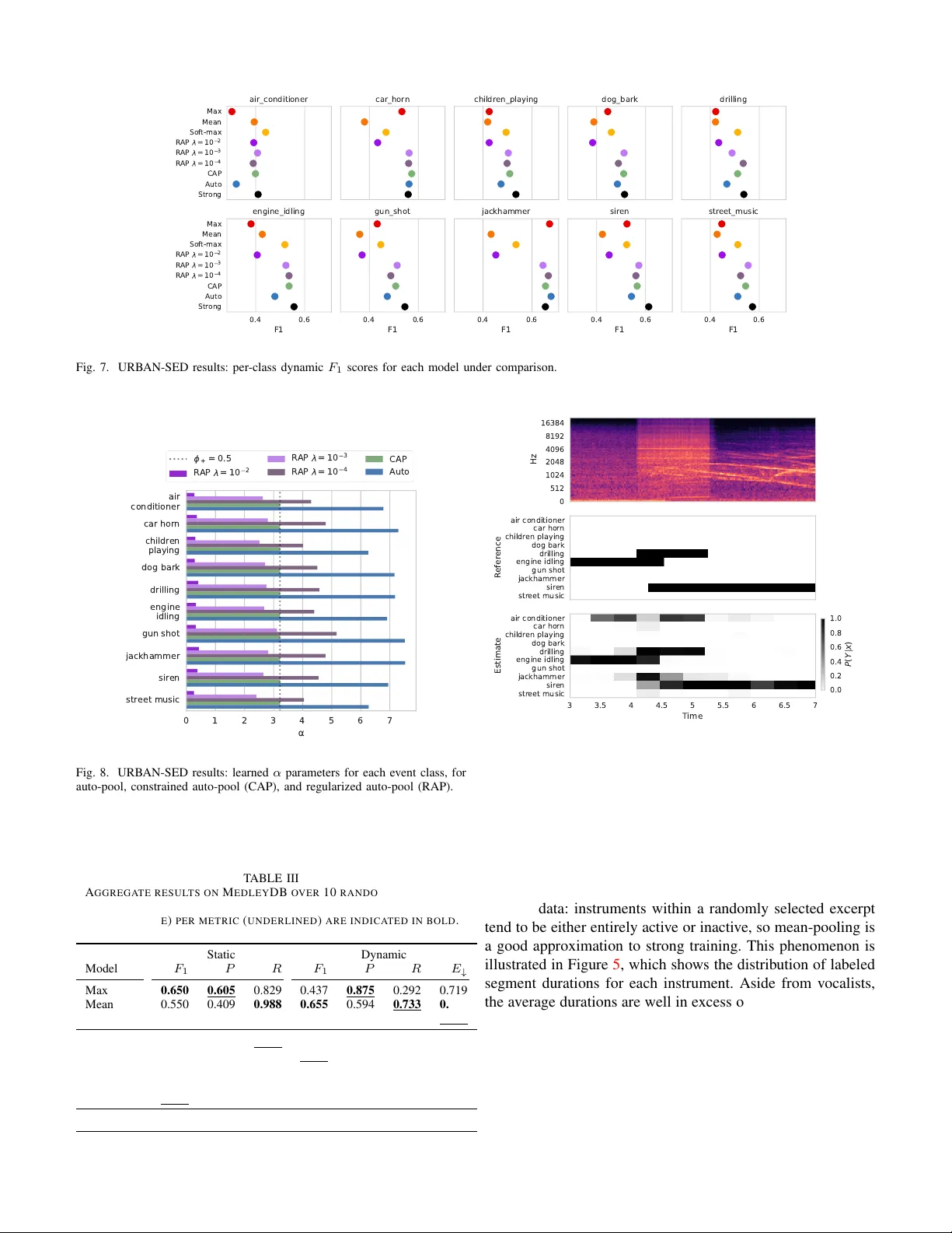
IEEE TRANSA CTIONS ON A UDIO, SPEECH AND LANGU A GE PR OCESSING, IN PRESS, 2018 1 Adapti v e pooling operators for weakly labeled sound e vent detection Brian McFee 1 , 3 , Justin Salamon 1 , 2 , Juan Pablo Bello 1 Senior Member , IEEE Copyright c  2018 IEEE. Personal use of this material is permitted. Permission from IEEE must be obtained for all other uses. Abstract —Sound event detection (SED) methods are tasked with labeling segments of audio recordings by the presence of active sound sources. SED is typically posed as a supervised machine learning pr oblem, requiring str ong annotations f or the presence or absence of each sound source at every time instant within the recording . However , strong annotations of this type are both labor- and cost-intensive for human annotators to produce, which limits the practical scalability of SED methods. In this work, we treat SED as a multiple instance learning (MIL) problem, where training labels are static over a short excerpt, indicating the presence or absence of sound sources but not their temporal locality . The models, howe ver , must still produce temporally dynamic predictions, which must be aggregated (pooled) when comparing against static labels during training. T o facilitate this aggregation, we de velop a family of adaptive pooling operators—r eferred to as auto-pool—which smoothly interpolate between common pooling operators, such as min-, max-, or average-pooling, and automatically adapt to the characteristics of the sound sources in question. W e evaluate the proposed pooling operators on three datasets, and demonstrate that in each case, the proposed methods outperform non-adaptive pooling operators for static prediction, and nearly match the performance of models trained with strong, dynamic annotations. The proposed method is evaluated in conjunction with con volutional neural networks, but can be readily applied to any differentiable model for time-series label prediction. While this article f ocuses on SED applications, the pr oposed methods are general, and could be applied widely to MIL problems in any domain. Index T erms —Sound event detection, machine learning, mul- tiple instance learning, deep learning I . I N T RO D U C T I O N S OUND event detection (SED) is the task of automatically identifying the occurrence of specific sounds in continuous audio recordings. Gi ven a target set of sound sources of interest, the goal is to return the start time, end time, and label (the class) of every sound ev ent in the target set. SED is a key component in a number of technologies and applications emerging from the recent advances in machine learning and Internet of Things (IoT) technology such as noise monitor- ing for smart cities [ 1 ], bioacoustic species and migration monitoring [ 2 – 4 ], self-dri ving cars [ 5 ], surveillance [ 6 , 7 ], healthcare [ 8 ], and large-scale multimedia indexing [ 9 ]. Modern SED systems are typically implemented by super - vised machine learning algorithms, which are used to learn the parameters of a function to map a sequence of audio data to a sequence of ev ent labels. Because SED systems are required to 1 Music and Audio Research Laboratory 2 Center for Urban Science and Progress 3 Center for Data Science New Y ork University , New Y ork, USA produce dynamic (time-varying) label estimates at each instant within a recording, they are often trained from str ongly labeled training data , where the presence or absence of each source at each instant is known. While strongly labeled data is ideal for model dev elopment and ev aluation, it is also costly to acquire. As SED systems adopt data-intensiv e approaches—such as con volutional or recurrent neural networks—the availability and cost of strongly annotated data become serious impedi- ments to system development. If we are to accurately ev aluate the dynamic performance of SED systems, strongly labeled data is clearly necessary , and it is natural to assume that the same should hold for model de velopment. Howe ver , if one has access to a lar ger pool of data that has only been weakly labeled at a coarse time resolution ( e.g. , 10 second clips), it may be possible to learn a high-quality , dynamic predictor with lower annotation costs. The key to lev eraging this kind of weakly labeled data lies in the means by which dynamic predictions are aggregated or pooled across time to form static predictions. There are standard approaches to aggre gating predictions, such as max- or mean- pooling, which can be difficult to optimize (in the case of max ) or require strict assumptions about the characteristics of the data which may not hold in practice, e.g. , mean-pooling assumes that ev ent activ ation must occupy the majority of a labeled observ ation window . Making effecti ve use of weakly labeled data can therefore require substantial engineering and algorithm design effort. A. Our contributions In this article, we develop a general family of adaptiv e pooling operators—collectively referred to as auto-pool — which generalize and interpolate between standard operators such as max , mean, or min . The proposed methods are designed to be jointly learned with dynamic prediction models ( e.g . , conv olutional networks), allo wing dynamic predictors to be trained from weakly annotated data, and require minimal assumptions about the label characteristics. W e e v aluate the proposed methods on three multi-label, sound e vent detection datasets, which exhibit dif fering characteristics of label spar- sity and duration. Our empirical results show that the proposed methods outperform standard, non-adaptiv e pooling operators, and the resulting models achie ve comparable accuracy to models trained from strongly labeled data. I I . R E L A T E D W O R K A. Sound event detection Sound e vent detection (SED) has seen a dramatic increase in interest from the research community over the past decade, IEEE TRANSA CTIONS ON A UDIO, SPEECH AND LANGUA GE PROCESSING, IN PRESS, 2018 2 as e videnced by the gro wing popularity and participation in the DCASE challenge [ 10 ] and the emergence of domain-specific SED systems, e.g. , for bioacoustic SED [ 11 ]. Early approaches relied on standard features (such as Mel-frequency cepstral coefficients) combined with standard machine learning algo- rithms, such as support v ector machines [ 12 – 14 ] or Gaussian mixture models (optionally with temporal smoothing) [ 15 – 18 ]. Other strategies include spectral decomposition methods and source separation models [ 19 – 26 ]. The most recent research on SED is dominated by deep (fully connected) neural net- works [ 27 ], con volutional networks [ 4 , 28 , 29 ], recurrent net- works [ 30 , 31 ], or con volutional-recurrent networks [ 32 , 33 ]. The aforementioned approaches rely on strongly labeled data, which as discussed in the introduction, limits their practi- cal applicability . While this limitation can be ov ercome in part through data synthesis [ 34 ], the problem has led researchers to in vestigate models for SED that can be trained from weak (static) labels. Interest in this problem formulation spiked with the release of AudioSet [ 35 ], which contains approximately 2 million 10-second Y ouT ube clips with weak audio labels, and the DCASE 2017 challenge [ 10 ]. One of the DCASE 2017 tasks (T ask 4) was based on a subset of AudioSet, and the problem was to develop models that can be trained on weak labels but produce strong ( i.e. , dynamic, time-varying) labels. Many of the subsequently published papers addressing SED using weakly labeled data (section II-C ) formulate the problem in the multiple instance learning (MIL) frame work. B. Multiple instance learning Multiple instance learning (MIL) was proposed in its mod- ern form by Dietterich et al. [ 36 ] as a supervised learning problem where a single binary class label is applied to a set ( bag ) of related examples (instances) in the training set. MIL problems naturally arise in a variety of application domains where precise labeling can be expensiv e, such as object recognition in computer vision. A label may be applied to an image indicating the presence of an object, while the “instances” to be classified are small patches within the image. Similarly , for SED, it may be more cost-effecti ve to label a relativ ely long clip for the presence of an ev ent, rather than each individual frame. The general MIL formulation has been broadly applied within computer vision [ 37 – 39 ], it has been relatively less common in audio applications. Mandel and Ellis [ 40 ] com- pared two support vector machine-based MIL algorithms [ 41 , 42 ] for classifying 10-second music excerpts (the instances) for which labels had been generated at the lev els of track, album, or artist. Their target vocab ulary included a mixture of genre, style, and instrumentation tags, and they found that the best-performing method was the MI-SVM algorithm [ 41 ], but that it was comparable to a naiv e baseline in which aggregated training labels were propagated to all constituent instances prior to training. Relatedly , W u et al. dev eloped a hierarchical generativ e model for music emotion recognition [ 43 ]. In their model, song labels are modeled as generating multiple instances of se gments , which in turn each generate multiple sentences (instances) which are jointly represented by text (lyrics) and acoustic features. While their generativ e model is trained on weakly labeled data, it does not provide a direct mechanism for inferring instance-level labels. In other related work, Briggs et al. [ 44 ] compared se veral previously de veloped MIL algorithms for detecting (multiple) bird species from short (10–15s) audio excerpts. Their results demonstrated that k-nearest-neighbor [ 45 ] and clustering [ 46 ] approaches both perform well at excerpt-le vel prediction, but they did not report ev aluations at the level of instances (time- frequency patches). For comparison purposes, we ev aluate the methods proposed here on both static and dynamic prediction. C. Sound event detection using weakly labeled data When re viewing approaches for weakly labeled SED, we can group approaches by two key features: the model used to produce dynamic features (or predictions), i.e. , an instance- lev el representation, and the approach used to aggregate instance-lev el features or predictions to a bag-lev el (static) prediction. Note that for SED, instances typically correspond to audio frames or short chunks. In terms of modeling, while approaches based on GMM [ 47 ] and SVM [ 48 ] hav e been proposed, the vast majority are based on deep neural networks including DNN [ 49 ], CNN [ 50 – 54 ], RNN [ 55 ] and CRNN [ 56 ]. Some approaches propagate the bag-le vel label to all instances and train against these directly [ 51 , 56 ], which can introduce instance-lev el label noise. Other approaches are based on source separation, and obtain dynamic labels by post-processing the separated sources ( e.g. , by computing the frame-wise energy of each separated source) [ 57 , 58 ]. Howe ver , the majority of approaches aggregate instance- lev el representations over time to produce a bag-le vel predic- tion. Giv en the standard MIL formulation, it is understandable that most approaches rely on pooling or customized loss functions that make use of the max operator [ 47 , 48 , 50 ], though variants including (a precursor to this work) soft-max pooling [ 52 ], and mean pooling [ 53 ] have been proposed. As shall be discussed in Section III , max-pooling causes a number of issues that limit its efficac y as a pooling strategy for MIL. D. Attention and dif fer entiable pooling Attention mechanisms [ 59 ] have been recently de veloped as a way to restrict the dependence of an output prediction to a subset of the input. T ypically , attention mechanisms are applied to structur ed pr ediction problems, such as machine translation or automatic speech recognition, where the output is a sequence ( e.g. , predicted translation text) has some regular structure that may be exploited by the model architecture, which is often a recurrent neural network. While the basic idea of attention for MIL is appealing, the training labels in MIL are typically unstructured : e.g. , a single label that applies to an entire sequence. Ho we ver , the model must still produce structured predictions, and it is not directly ob vious how to apply standard attention mechanisms. Con volutional (feed-forward) attention [ 60 ] is a closer fit to the MIL setting, as the attention mechanism is used to summarize a structured input by a fix ed-length context vector c as a weighted average c = P t e t h t of instance representations IEEE TRANSA CTIONS ON A UDIO, SPEECH AND LANGUA GE PROCESSING, IN PRESS, 2018 3 { h t } , from which the output is predicted as ˆ y = g ( c ) . Note that the intermediate representations h t do not generally constitute instance predictions. Because g is usually non-linear (and non- con vex), there is no direct relationship between the attention- aggregated output g ( c ) = g ( P t e t h t ) , the weighted av erage of g applied to instances P t e t g ( h t ) , and instance-wise outputs g ( h t ) . As a result, while optimizing g ( c ) may provide a good bag-lev el model, it does not directly provide an instance-le vel model as required by MIL. Recently , attention-based models have been proposed which use class likelihoods as intermediate representations, along with an identity mapping for g [ 49 , 54 ]. The methods we dev elop in this article are similar in spirit, but with a more constrained and interpretable attention mechanism that relates directly to the instance-lev el predictions and the MIL problem formulation. Moreov er, the proposed methods introduce only a single additional parameter for each class, which can be directly interpreted as interpolating between different standard pooling operators, as described below . Aside from attention models, similar techniques ha ve been used to provide dif ferentiable pooling operators for MIL. Most similar to the methods we propose is that of Hsu et al. [ 39 ], which uses the smooth log P exp approximation to the max operator for MIL applications in computer vision. Hsu et al. introduce a hyper -parameter to control the sharpness of the approximation, but it is fixed a priori, and unlike the methods proposed here, the aggregation does not adapt automatically . Moreov er , because log P exp aggregation is non-linear, it ex- hibits similar difficulty in recovering instance-wise predictions as the attention-based approach described abo ve. Finally , Zeiler and Fergus [ 61 ] dev eloped a general formu- lation that adaptiv ely interpolates between different standard pooling operators. Although this approach has been applied to audio problems [ 62 ], its use has been limited to pooling of internal feature representations in con volutional networks, and it has not been used in MIL applications. The methods we dev elop in this article are conceptually simpler , and more lim- ited in scope to directly address the dif ficulties of aggregating predictions in MIL problems. I I I . M E T H O D S In this section, we describe the multiple instance learning problem in general, and illustrate short-comings of standard pooling operators when applied to the MIL context. W e then dev elop a family of adaptive pooling operators to reduce dynamic label predictions to static predictions during training. For ease of exposition, we first deriv e the methods for single- label binary classification problems, followed by the general- ization to multi-label settings. A. Multiple instance learning In the multiple instance learning (MIL) problem formu- lation, training data are provided as labeled sets ( bags ) of examples ( X i , Y i ) n i =1 where X i = { x 1 , x 2 , · · · } ⊂ X contains multiple instances x j , and Y i ∈ { 0 , 1 } is a single label for the set X i [ 36 ], and X and Y denote the feature and label spaces. The label con vention is that Y i = 1 if any instance x ∈ X i is positiv e, and Y i = 0 if all instances are negati ve. The goal is Fig. 1. Pooling operators propagate gradient information in proportion to the responsibilities they assign to instance-level predictions, indicated here by the darkness of arrows. Left: max assigns all responsibility to the largest instance; middle: mean assigns equal responsibility to all instances; right: soft-max (eq. ( 6 )) assigns greater responsibility to large instances. to use this weakly labeled data to learn an instance classifier h : X → Y . While MIL can be applied to a variety of learning al- gorithms ( e.g . , support vector machines or nearest neighbor classifiers), in this work we focus on deep neural networks. The classifiers under consideration here take the form of a thresholded likelihood ˆ p ( Y | x ) , e.g. , h ( x ) = ( 1 ˆ p ( Y | x ) ≥ 0 . 5 0 otherwise . (1) In this formulation, the predicted label for a bag is the maxi- mum ov er instance-wise predictions. Equiv alently , a likelihood for the bag-label can be induced from the instance likelihoods by defining the bag-level likelihood as ˆ P ( Y | X ) = max x ∈ X ˆ p ( Y | x ) , (2) which results in the bag prediction rule h ( X ) = ( 1 ˆ P ( Y | X ) ≥ 0 . 5 0 otherwise . (3) This prediction rule is depicted schematically in Figure 1 (left), where the bag-level prediction depends only on the maximum of its instance-lev el predictions. During training, the objectiv e is to maximize the likelihood of observed labeled bags, e.g . , by minimizing the binary cross- entropy ov er the model parameters θ : min θ 1 n n X i =1 − Y i log ˆ P ( Y | X i ) − (1 − Y i ) log  1 − ˆ P ( Y | X i )  . (4) B. Max-pooling T ypically , eq. ( 4 ) is optimized by some form of gradient descent, which requires propagating gradients through the max operator in eq. ( 2 ) via the chain rule. The max operator is not itself differentiable, so sub-gradient descent must be used instead. The sub-differ ential set of the max operator applied to inputs { z i } ⊂ R is the set of all conv ex combinations of its maximizers’ s sub-gradients (assuming each input is sub- differentiable): ∂ max { z i } = Con v  g     g ∈ ∂ z i ∧ z i = max j z j  (5) IEEE TRANSA CTIONS ON A UDIO, SPEECH AND LANGUA GE PROCESSING, IN PRESS, 2018 4 where Con v ( S ) denotes the conv ex hull of a set S : Con v ( S ) = ( X x ∈ S µ x x      X x ∈ S µ x = 1 ∧ ∀ x µ x ≥ 0 ) . Any element of ∂ max can be used in place of a gradient, though most implementations select a single maximizer at random; often, the maximizer is unique, so the distinction is unimportant. A sub-gradient of max can be thus viewed as a weighted average of all inputs, subject to the constraint that non-maximizing inputs must have weight 0. When applying the chain rule to ∂ max , the sub-gradient of the objecti ve function with respect to non-maximizing instances is 0, and those instances therefore do not contribute when updating the parameters θ . This is particularly problem- atic early in training, where the instance-wise predictions are essentially random. Parameter updates then depend entirely upon single, randomly selected instances (as depicted in Fig- ure 1 , left). As a result, max-pooling for MIL can be sensitive to initialization, generally unstable, and dif ficult to deploy. C. Soft-max pooling T o ameliorate the issues highlighted above, we proposed in previous work [ 52 ] to replace the max operator in eq. ( 2 ) by the soft-max weighted average : ˆ P s ( Y | X ) = X x ∈ X ˆ p ( Y | x )     exp ˆ p ( Y | x ) X z ∈ X exp ˆ p ( Y | z )     . (6) This operator behaves similarly to the max operator , in that ˆ P s is large if any of its inputs ˆ p ( Y | x ) are large, and small if all of its inputs are small. Howe ver , it is continuously differentiable, and assigns responsibility to each instance x so that the entire bag contrib utes to the gradient calculation and parameter updates. As illustrated in Figure 1 (right), each instance x contributes in proportion to its label likelihood ˆ p ( Y | x ) , so that positi ve predictions hav e more influence and negati ve predictions have less. Because the inputs to the soft-max pooling operator are probabilities ˆ p ( Y | x ) ∈ [0 , 1] , the weights assigned by eq. ( 6 ) are also bounded. In general, we have the follo wing relation between a soft-max’ s input and output: Proposition 1. Let a ≤ b ∈ R and z ∈ [ a, b ] m ⊂ R m , and let ρ ( z ) i := exp( z i ) / P j exp( z j ) denote the soft-max operator . Then for any coor dinate i , the corr esponding soft-max output ρ ( z ) i is bounded as e a e a +( m − 1) · e b ≤ ρ ( z ) i ≤ e b e b +( m − 1) · e a . Pr oof. First, observe that ρ ( z ) i is proportional to exp z i and in versely proportional to P j 6 = i exp z j . A soft-max coordinate ρ ( z ) i is therefore maximal when one coordinate z i = b is maximal, and all remaining ( m − 1) coordinates z j 6 = i = a 10 20 30 40 50 60 70 80 90 100 B a g s i z e ( m ) 0.0 0.1 0.2 Instance weight Uniform weights Soft-max bounds Fig. 2. The soft-max weighted average (eq. ( 6 )) produces instance weights satisfying the bounds giv en in eq. ( 7 ) (shaded region). As the size m of the bag grows, the bounds conv erge to 1 /m (solid line). are minimal. In this case, the soft-max output ρ ( z ) for each coordinate k is ρ ( z ) k = exp( z k ) e b +( m − 1) · e a . Since all z k ≤ b , this achie ves the upper bound. A similar argument proves the analogous lower bound. Applying proposition 1 , if a bag has | X | = m instances, and each instance x ∈ X has a likelihood 0 ≤ ˆ p ( Y | x ) ≤ 1 , then the weight for each instance is bounded as 1 1 + e · ( m − 1) ≤ exp ˆ p ( Y | x ) X z ∈ X exp ˆ p ( Y | z ) ≤ e e + m − 1 . (7) Soft-max pooling therefore has limited capacity to concentrate on a small portion of instances within a bag, since the weight for any single instance is Θ(1 /m ) . As illustrated in Figure 2 , soft-max pooling behav es similarly to unweighted av eraging as the bag size grows. D. Auto-pooling The bounded range problem of soft-max pooling can be addressed by introducing a scalar parameter α ∈ R : ˆ P α ( Y | X ) = X x ∈ X ˆ p ( Y | x )     exp ( α · ˆ p ( Y | x )) X z ∈ X exp ( α · ˆ p ( Y | z ))     . (8) T reating α as a free parameter to be learned along-side the model parameters θ allows eq. ( 8 ) to automatically adapt to and interpolate between different pooling behaviors. For example, when α = 0 , eq. ( 8 ) reduces to an unweighted mean (Figure 1 , center); when α = 1 , eq. ( 8 ) simplifies to soft-max pooling eq. ( 6 ); and when α → ∞ , eq. ( 8 ) approaches the max operator . W e therefore refer to the operator in eq. ( 8 ) as auto-pooling . W ith auto-pooling, for α ≥ 0 , the bounds from proposition 1 are [ a, b ] = [0 , α ] , and the instance weights are bounded by 1 1 + e α · ( m − 1) ≤ exp ( α · ˆ p ( Y | x )) X z ∈ X exp ( α · ˆ p ( Y | z )) ≤ e α e α + m − 1 , (9) which approaches the open unit interv al (0 , 1) as α → ∞ . IEEE TRANSA CTIONS ON A UDIO, SPEECH AND LANGUA GE PROCESSING, IN PRESS, 2018 5 Additionally , letting α ≤ 0 leads to approximate min - pooling, where smaller input values recei ve larger weight in the combination. In this case, the bounds are [ a, b ] = [ α, 0] , and the resulting instance weight bounds are: e α e α + m − 1 ≤ exp ( α · ˆ p ( Y | x )) X z ∈ X exp ( α · ˆ p ( Y | z )) ≤ 1 1 + e α · ( m − 1) . (10) As α → −∞ , the weight bounds again approach the unit interval (0 , 1) , except that the upper bound is now achieved by the smallest instance prediction. This effecti vely relaxes the core assumption of multiple instance learning that a bag label is equal to the max (disjunction) over instance labels. Supporting min (conjunction) behavior allows for a bag to be predicted as a positiv e example if all of its instances are predicted as positiv e examples, which would be appropriate for long-duration ev ents. E. Constrained auto-pooling Equation ( 9 ) bounds the effecti ve range of the weight as- signed to any given instance in terms of the pooling parameter α and the bag size m . Howev er, in some applications, it may be more natural to constrain α in terms of the amount of weight the pooling operator is allowed to assign to a single instance when making a bag-lev el decision. For example, in sound event detection, this may correspond to requiring the detector to be active for at least some minimum time duration for the bag to be predicted as a positiv e example. Alternately , one may require that a minimum fraction of instances must be positiv e before the bag is predicted positiv e, or equiv alently , that no single instance receives too much weight in ( 8 ). Let 1 /m ≤ φ + < 1 denote the maximum permissible aggregation weight for a single instance. 1 Then α ≥ 0 can be upper-bounded as: e α e α + m − 1 ≤ φ + ⇒ α ≤ ln φ + 1 − φ + + ln ( m − 1) . (11) Similarly , a minimum weight constraint 0 < φ − ≤ 1 /m produces the following lo wer bound for α : φ − ≤ e α e α + m − 1 ⇒ α ≥ ln φ − 1 − φ − + ln ( m − 1) . (12) Note that these bounds are tight, in that φ − = φ + = 1 /m implies α = 0 , which recovers mean-pooling. Now , consider the minimal upper bound φ + that allows a single instance to determine the majority vote for a bag. This is achiev ed by the extremal case where one instance i is maximal and the remaining instances j 6 = i are minimal: ˆ p ( Y | x k ) = ( 1 k = i 0 k 6 = i . (13) W ith the decision rule (and threshold) given in eq. ( 3 ), φ + = 0 . 5 is the minimal upper bound on weights that produces max-pooling behavior , and therefore constitutes an upper 1 The maximum weight φ + cannot be less than 1 /m because all weights must sum to 1. Similarly , a minimum weight bound φ − cannot exceed 1 /m . bound that does not significantly reduce the flexibility of auto- pooling. W ith this value of φ + , eq. ( 11 ) simplifies to φ + = 0 . 5 ⇒ α ≤ ln( m − 1) . Throughout the remainder of this article, we will refer to auto- pooling with the φ + = 0 . 5 bound imposed as constrained auto-pool (CAP) . F . Re gularized auto-pooling As an alternati ve to constrained auto-pool, one may consider r egularized auto-pool (RAP) , where a penalty is applied to α to pre vent it from placing too much weight on individual instances b ut without an explicit bound on the maximum (or minimum) weight. While there are many possibilities for the choice of penalty function, here we opt for a quadratic penalty α 2 , so that the penalty grows with α . This promotes mean- like behavior , but still provides flexibility to learn max-pooling behavior if necessary . Concretely , for the remainder of this article, we will denote by RAP any auto-pool model with a quadratic penalty: min θ,α f ( θ ) + λ | α | 2 , where f ( θ ) denotes the learning objectiv e of eq. ( 4 ), and λ > 0 is a positi ve coefficient. For multi-label formulations, the penalty generalizes to the squared Euclidean norm λ k α k 2 . G. Multi-label learning The discussion so far has centered on binary classification problems, but the methods directly generalize to multi-label settings, in which each instance x receiv es multiple positive labels. In this setting, a separate auto-pooling operator is applied to each class. Rather than a single parameter α , there is a vector of parameters α c where c index es the output vocab ulary . This allows a jointly trained model to adapt the pooling strategies independently for each category . I V . E X P E R I M E N T S In this section, we describe a series of experiments inv es- tigating the behavior of auto-pooling methods on three sound ev ent detection applications: urban environments (URBAN- SED), smart cars (DCASE 2017), and musical instru- ments (MedleyDB). For each dataset, we compare models trained with standard, non-adapti ve pooling operators ( max and mean), the soft-max pooling model described in Sec- tion III , and the three adaptive methods: auto-pool, con- strained auto-pool (CAP), and regularized auto-pool (RAP). For RAP models, we report results independently for λ ∈ { 10 − 2 , 10 − 3 , 10 − 4 } . For the urban en vironment and musical instrument applications, we will also compare to a model trained with strong (time-varying) labels to provide a sense of the maximum expected performance for the given model ar- chitecture. Models trained with strong labels omit the temporal pooling step, and the training loss is computed independently for each instance. The smart car dataset (DCASE 2017) does not provide strong labels for the training set, so this comparison could not be performed. IEEE TRANSA CTIONS ON A UDIO, SPEECH AND LANGUA GE PROCESSING, IN PRESS, 2018 6 W e report standard ev aluation metrics for both static (bag- lev el) and dynamic (segment-lev el) prediction: precision, re- call, and F 1 . 2 For static predictions the metrics are computed following the standard methodology for multi-label classifi- cation ev aluation. For the dynamic predictions we compute the segment-based variant of the aforementioned metrics as defined by Mesaros et al. [ 63 ] using a segment duration of 1 second, as per the DCASE challenge [ 10 ]. Additionally , for the dynamic prediction task, we report the err or rate E , defined as the av erage number of substitutions, insertions, and deletions of events over all segments. Note that precision, recall and F 1 range from 0 (worst) to 1 (best), while the error rate E is non-negati ve with 0 being the best and greater v alues representing worse performance. A. Datasets 1) URBAN-SED: URB AN-SED is a dataset of 10,000 soundscapes generated using the Scaper soundscape synthesis library [ 34 ]. Each soundscape has a duration of 10 s, and the dataset as a whole totals 27.8 hours of audio with close to 50,000 annotated sound events from 10 sound classes. Each soundscape contains between 1–9 foreground sound ev ents, where the source material for the ev ents comes from the UrbanSound8K dataset [ 64 ], and has a background of Brownian noise resembling the typical “hum” often heard in urban en vironments. The dataset comes pre-sorted into train, validation and test splits containing 6000, 2000 and 2000 soundscapes respectiv ely . An important characteristic of URBAN-SED is that since both the audio and annotations were generated computa- tionally , the annotations are guaranteed to be correct and complete, while the dataset is an order of magnitude larger than the largest strongly labeled SED dataset compiled via manual labeling. Since the soundscapes are “composed” using a process akin to an audio sequencer , they are not as realistic as manually labeled datasets of real soundscape recordings. In particular , as illustrated in Figure 3 , ev ents may be artificially truncated in duration in unnatural-sounding ways. Still, it has been shown that the data still present a challenging scenario for state-of-the-art SED models [ 34 ]. 2) DCASE 2017 T ask 4: The DCASE 2017 challenge [ 10 ] consisted of four tasks, including one task with the same problem formulation as this work (training a model to generate strong predictions from weakly labeled training data), task 4: “Large-scale weakly supervised sound ev ent detection for smart cars”. The dataset used for this task is a subset of the AudioSet dataset [ 35 ], and consists of just over 50K 10- second excerpts from Y ouT ube videos. The dataset is split into a “de velopment” set of 51660 e xcerpts and an “ev aluation” ( i.e. , test) set of 1103 excerpts. The dev elopment set is further divided into a “train” set with 51172 excerpts and a v alidation 2 F 1 -macro reports the unweighted average of class-wise F 1 scores. Micro- av erages are not av ailable for segment-based ev aluation. 0 2 4 6 8 10 Event duration (seconds) air conditioner car horn children playing dog bark drilling engine idling gun shot jackhammer siren street music Fig. 3. Event durations for each class in the URBAN-SED. Each point corresponds to a test clip, and the mean event durations are indicated by vertical bars. By construction, each event is clipped to at most 3 s (30% of the clip), though an ev ent class can occur multiple times within a clip. set of 488 videos. 3 For conciseness, for the remainder of the paper we shall refer to this dataset simply as “DCASE 2017”. The sound ev ents in this dataset come from 17 sound classes selected by the challenge organizers out of the AudioSet ontology [ 35 ] that are related to traffic such as sirens, horns, beeps, and different types of vehicles such as car , bus and truck. The weak labels were generated semi-automatically [ 35 ], while strong labels for the v alidation and test sets were manually annotated by the challenge organizers by listening to the audio (without watching the video). The dataset fits our problem formulation, but its annotations ha ve limitations, which makes proper ev aluation difficult. Not all target sound ev ents are guaranteed to be labeled and ha ve a non-zero duration, and some such as “car” and “car passing by” are semantically ov erlapping. Ho wever , it does hav e a unique distribution of ev ent durations compared to the other two datasets used in this study . The event durations for this dataset, depicted in Figure 4 , follo w a more natural distribution than those of URB AN-SED (Figure 3 ), which we expect to influence the behavior of the proposed models, in particular the auto-pool models where α is learned from the data. Our moti v ation for including this dataset in the ev aluation is primarily to study the adapti ve behavior of the α parameter , and not to achie ve the best possible performance (measured by F 1 ). 4 3) MedleyDB: MedleyDB [ 65 ] is a collection of 122 multi- track recordings from a variety of musical genres and styles. 3 T o av oid possible confusion it is necessary to highlight the difference between the nomenclature used in the challenge and the nomenclature more commonly found the literature, as the latter will be used in this study for consistency . Throughout this paper, we use the challenge “train” set as our training set, the challenge “test” set as our validation set, and the challenge “ev aluation” set as our test set. 4 For a thorough ev aluation of existing methods on this dataset, we refer interested readers to the DCASE 2017 challenge results: https://www .cs.tut.fi/ sgn/arg/dcase2017/challenge/task- lar ge- scale- sound- ev ent- detection- results . IEEE TRANSA CTIONS ON A UDIO, SPEECH AND LANGUA GE PROCESSING, IN PRESS, 2018 7 0 2 4 6 8 10 Event duration (seconds) Air horn, truck horn Ambulance (siren) Bicycle Bus Car Car alarm Car passing by Civil defense siren Fire engine, fire truck (siren) Motorcycle Police car (siren) Reversing beeps Screaming Skateboard Train Train horn Truck Fig. 4. Event durations for each class in DCASE 2017. Each point corresponds to a test clip, and the mean e vent durations are indicated by vertical bars. DCASE events typically cov er at least 40% (4 s) of the clip, and the high concentrations at 10.0 indicate that ev ents often span the entire clip. While it was initially developed to facilitate pitch tracking ev aluation, it includes time-varying instrument activ ation la- bels for each track. Because each track in MedleyDB is provided in the form of isolated instrument recordings ( stems ), it is possible to gen- erate dif ferent mixtures of the stem recordings for an y gi ven track. This motiv ates a form of data augmentation: if a track has n instruments, we generate n alternate mix es, where mix i has the i th instrument removed; the remaining n − 1 stems are linearly mixed to best approximate the full mix, using the mixing coefficients provided by the MedleyDB python package. 5 By training on this expanded set of leave-one- out mixes, we separate each instrument from its surrounding context, which helps to eliminate confounding factors when estimating the presence of each instrument. The expanded MedleyDB set contains 531 tracks, totaling 33.1 hours of audio. Because of the skewed distribution of instruments in Med- leyDB, we reduced the v ocabulary of interest to the 8 most common sources: acoustic guitar , clean electric guitar , dis- torted electric guitar , drum set, electric bass, female singer , male singer , piano . Unlike URBAN-SED and DCASE, there is not a pre-defined ev aluation split of MedleyDB. W e instead repeated the experiment over 10 random, artist-conditional 80–20 train-test splits; validation sets were randomly split 80–20 from the training splits (without artist conditioning). Having multiple train-test splits allo ws us to perform statistical analyses which are not possible with the URB AN-SED and DCASE datasets. W e therefore do not make claims as to which methods perform “best” on URBAN-SED and DCASE. Figure 5 illustrates the distribution of instrument activ ation 5 https://github .com/marl/medleydb 1 0 0 1 0 1 1 0 2 Event duration (seconds) acoustic guitar clean electric guitar distorted electric guitar drum set electric bass female singer male singer piano Fig. 5. Event durations for each class in MedleyDB (logarithmically scaled). Each point corresponds to the total duration of an instrument ov er a track, with the mean durations indicated by vertical bars. The black line marks the 10 second point used to generate training patches. durations over the dataset. Most instruments are active for substantially longer than the 10 s observ ation window used in our experiments, indicating that labels should be expected to be constant (entirely on or entirely off) over the duration of a training example. B. Model arc hitectur e The model used in this work is divided into two main components: a dynamic predictor that generates predictions at a fine temporal resolution ( i.e. , frame/instance-lev el pre- dictions), and a pooling layer which aggregates the instance- lev el predictions into a single static (bag-le vel) prediction. Our goal is to compare and contrast the different pooling functions proposed in Section III . As such, in this w ork we adopt a single model architecture for the dynamic predictor , and keep it fixed throughout the study . A block diagram depicting the complete architecture including the dynamic predictor follo wed by the temporal pooling layer is provided in Figure 6 . For the dynamic predictor, we use an architecture inspired by the audio subnetwork of the L 3 -Net architecture proposed by Arandjelovic and Zisserman [ 66 ], which was shown to learn highly discriminativ e deep audio embeddings from a self-supervised audio-visual correspondence task. In this work the input dimensions are ordered as (feature, time); details about the input are provided in Section IV -C . The model begins with four con volutional blocks, each block consisting of tw o conv olutional layers follo wed by strided (2 , 2) max- pooling, where the number of conv olutional filters is doubled for each subsequent block (16 , 32 , 64 , 128) and all filters are of dimensionality (3 , 3) . This is followed by a single con volutional layer with 256 full-height (8 , 1) filters, followed by a single dense layer applied independently to each time- step, and with as many outputs (units) as there are classes in the dataset being used. Batch normalization [ 67 ] is applied to the output of ev ery con volutional layer as well as to the input to the network. W e apply dimensionality-maintaining padding (“same padding”) to the input to all conv olutional IEEE TRANSA CTIONS ON A UDIO, SPEECH AND LANGUA GE PROCESSING, IN PRESS, 2018 8 Batch normalization Conv: 16 (3, 3) Conv: 16 (3, 3) P ool: (2, 2) Time Distributed Dense: n_classes T emporal Pooling Input: log-mel spectrogram Output 1: time-var ying per -class likelihoods (str ong labels) Output 2: weak labels Conv: 32 (3, 3) Conv: 32 (3, 3) P ool: (2, 2) Conv: 64 (3, 3) Conv: 64 (3, 3) P ool: (2, 2) Conv: 128 (3, 3) Conv: 128 (3, 3) P ool: (2, 2) Conv: 256 (8, 1) Fig. 6. Block diagram of the model architecture used in this study , including its two main components: a fully conv olutional dynamic predictor , followed by a temporal pooling layer implemented by any of the pooling functions described in Section III : max, mean, soft-max, auto-pool, constrained auto-pool (CAP) or regularized auto-pool (RAP). layers but the last, where we do not apply padding (“valid padding”). W e use rectified linear unit (ReLU) activ ations for all conv olutional layers and sigmoid activ ations for the output layer to support multi-label classification. The output of the latter is a multi-label prediction ˆ p ( Y | x ) for each frame (instance) x . Note that since the model down-samples in time by max-pooling, the frame rate of the dynamic predictions is reduced by a factor of 16 from the input. Finally , the output of the dynamic predictor is aggregated ov er all instances using one of the pooling operators presented in Section III to produce a static prediction ˆ P ( Y | X ) for each class, represented in Figure 6 by the temporal pooling layer at the right end of the diagram. Note that since the dynamic predictor is composed of con volutional layers and a single time-distributed dense layer , it is agnostic of the input length ( i.e. , the number of input instances/frames). This is followed by the temporal pooling layer which is again agnostic of the input length. As such, the entire architecture is length-agnostic (for audio, duration- agnostic) and can accept input of arbitrary length. That said, some of the pooling functions presented in Section III are affected by the length of the input: e.g. , soft-max pooling approaches mean pooling as the length of the input increases, and the parameter α for auto-pooling methods depends on the bag length m . Howe ver , this only matters for static prediction, and after the model has been trained, it can still produce dynamic predictions on arbitrary-length inputs. C. T raining and evaluation In all experiments, training data was augmented using MUD A [ 68 ] to generate pitch-shifted v ersions of each e xample by {± 1 , ± 2 } semitones, increasing the ef fectiv e training set size by a factor of 5. All signals were processed with librosa 0.5.1 [ 69 ] to produce log-scaled Mel spectrograms with the following parameters: sampling rate 44.1 KHz, n FFT = 2048 (46ms windows), hop length of 1024 samples (frame rate of 43 Hz), and 128 Mel frequency bands. The models produce dynamic predictions at a frame rate of 43 / 16 ≈ 2 . 69 Hz. Models were implemented using Keras [ 70 ] and T ensor- Flow [ 71 ]. Each model was trained using the Adam opti- mizer [ 72 ], with data sampled using Pescador 1.1 [ 73 ]. Models were trained on mini-batches of 16 10-second patches. Early stopping was used if the v alidation accuracy did not improve for 30 epochs; learning rate reduction was performed if the validation accuracy did not improve for 10 epochs. Auto-pool models (including CAP and RAP) were initialized with α = 1 . All models were ev aluated using the sed ev al package [ 63 ] to compute segment-based metrics with the se gment duration set to 1 s as per the DCASE 2017 challenge ev aluation. For comparison purposes, we report accuracy for static (bag-lev el) prediction accuracy using the decision rule given in eq. ( 3 ), i.e. , the maximum ov er dynamic predictions. When training on the MedleyDB dataset, training samples were generated by randomly sampling 10 second excerpts from the full-duration songs. The bag label for each excerpt was considered positiv e for any instruments which were activ e for at least 10% (1 s) of the excerpt, to match the 1 s duration used for the segment-based ev aluation. For reproducibility , we make our implementation and ex- periment framework software used in this study publicly av ailable. 6 T o enable easy use of the proposed auto-pool function in new work, we have also implemented it as an independent Keras layer . 7 V . D I S C U S S I O N This section describes the results of the experimental ev al- uation, broken down by data-set. A. URBAN-SED r esults T able I presents the results of the URB AN-SED ev aluation, av eraged across all classes. On the static prediction task, auto- pool achiev es the highest F 1 score of all MIL models under comparison, although the constrained and regularized v ariants are nearly equivalent. Note that the strong model, trained with full access to time-v arying labels, performs only slightly better , indicating that the auto-pool is ef fective for static prediction. This trend carries ov er to the dynamic prediction task, where the constrained auto-pool model (CAP) achiev es F 1 = 0 . 533 , compared to the strong model’ s F 1 = 0 . 551 , and compa- rable scores are achieved by the regularized models with λ ∈ { 10 − 3 , 10 − 4 } . On this dataset, the auto-pool model 6 https://github .com/marl/milsed 7 https://github .com/marl/autopool IEEE TRANSA CTIONS ON A UDIO, SPEECH AND LANGUA GE PROCESSING, IN PRESS, 2018 9 T ABLE I C L AS S - AG G RE G A T ED R E S U L T S O N U R BA N - SE D . Static Dynamic Model F 1 P R F 1 P R E ↓ Max 0.742 0.774 0.717 0.463 0.774 0.330 0.695 Mean 0.543 0.726 0.436 0.408 0.280 0.751 2.10 Soft-max 0.630 0.772 0.537 0.492 0.397 0.646 1.22 RAP 10 − 2 0.544 0.719 0.449 0.419 0.296 0.717 1.88 RAP 10 − 3 0.746 0.790 0.711 0.529 0.584 0.484 0.731 RAP 10 − 4 0.754 0.754 0.756 0.526 0.650 0.442 0.681 CAP 0.754 0.781 0.732 0.533 0.622 0.466 0.696 Auto 0.757 0.784 0.739 0.504 0.738 0.382 0.665 Strong 0.762 0.708 0.822 0.551 0.693 0.458 0.642 appears to over -fit the weak annotations, and a similar trend can be observed for the max -pooling model. Con versely , RAP with λ = 10 − 2 appears to be ov er-re gularized, and behav es similarly to mean-pooling on both static and dynamic prediction tasks. Figure 7 sho ws the F 1 scores independently for each class. While there is some variation across classes, RAP ( λ ≤ 10 − 3 ) and CAP consistently achieve high scores, and closely track the strong model. Mean and RAP ( λ = 10 − 2 ) tend to do poorly on ev ent classes which are transient or highly localized in time ( gun shot , car horn ). This is in accordance with Figure 1 : mean-pooling predictions of sparse event categories assigns equal responsibility to each frame in the input, which will be erroneous for any frames that do not cov er the e vent in question. The fact that RAP λ = 10 − 2 exhibits this beha vior indicates that the regularization term is too strong, and the model rev erts to mean pooling. Figure 8 illustrates the α vectors learned by each auto- pooling model. In particular , the CAP model learns to max- imize all α to the upper bound, indicating that max-like behavior is preferred for all classes. This is likely an artifact of how the dataset was constructed: e vents are artificially clipped to at most 3 seconds, which results in implicitly sparse class acti v ations for each bag (Figure 3 ). Note, ho wev er , that although the auto-pool models learn to produce max-like behavior , they consistently outperform the max -pool model on this dataset. This finding is consistent with the motiv ations for soft-max pooling given in Section III : max-pooling produces extremely sparse gradients during training, which impedes the model’ s ability to learn stable representations. By contrast, initializing the auto-pool model with α = 1 (softmax-like behavior) produces dense gradients early in training, which become sparser as the model con verges toward max-like behavior . Figure 9 illustrates the predictions made by the RAP model with λ = 10 − 3 on a validation clip. While the model does show some confusion ( engine idling and air conditioner , or drilling and jackhammer ), the temporal localization is gener- ally good. B. DCASE 2017 r esults T able II presents the class-aggregated results on the DCASE 2017 data. Note that because the DCASE training T ABLE II A G G R EG ATE R E S ULT S O N D C A S E 2 0 1 7 . Static Dynamic Model F 1 P R F 1 P R E ↓ Max 0.257 0.650 0.267 0.252 0.679 0.155 0.874 Mean 0.397 0.712 0.384 0.426 0.309 0.685 1.57 Soft-max 0.389 0.683 0.381 0.466 0.391 0.576 1.04 RAP 10 − 2 0.355 0.696 0.359 0.436 0.325 0.663 1.43 RAP 10 − 3 0.357 0.669 0.357 0.410 0.308 0.613 1.44 RAP 10 − 4 0.372 0.694 0.374 0.445 0.340 0.642 1.32 CAP 0.426 0.700 0.414 0.427 0.360 0.524 1.12 Auto 0.454 0.664 0.453 0.425 0.401 0.451 0.968 data only has clip-lev el annotations, we cannot compare to a baseline model trained on strong annotations. As before on URB AN-SED, the auto-pool method achieves the highest static F 1 score. Soft-max pooling achie ves the highest dynamic F 1 score (0.466), but both the mean and auto-pool methods are comparable, all landing in the range of 0.41–0.45. Notably , the max-pooling model substantially under - performs the competing methods on both static and dynamic prediction tasks. This holds uniformly across all per-class ev aluations, as illustrated in Figure 10 . W ith the exception of unconstrained auto-pool, the remaining models generally perform comparably across all classes. Figure 11 sho ws the learned α vectors for each auto- pool model. Unlike the URBAN-SED results in Figure 8 , auto-pool models do not uniformly approach max-pooling on the DCASE data. Instead, there is significant diversity among the different classes, with some tending toward max- pooling behavior (large α for screaming or air horn/truck horn , skateboar d ) and others tending toward mean-pooling behavior (small α for bus or car passing by , truck ). Referring to Figure 4 , the classes for which auto-pool (and CAP) learn large α tend to have short e vent durations. By contrast, the classes which result in small α values tend to span the majority of the clip, and have high concentration on full duration (1.0). In these classes, the bag- and instance-labels are equiv alent, so it is expected that mean-pooling (small α ) out-performs max -pooling. C. MedleyDB results T able III lists the class-aggregated scores ov er the Med- leyDB dataset. Follo wing Dem ˇ sar [ 74 ], the distributions of scores over all splits are compared using a Friedman test [ 75 ] with Bonferroni-Holm correction ( α = 0 . 05 ) [ 76 ], and meth- ods indistinguishable from the best (a verage) are indicated in bold. The strong model is omitted from statistical comparison, as we are primarily concerned with differentiating among MIL algorithms. From this analysis, we observe little differentiation between the various methods. Mean-pooling and RAP ( λ ≥ 10 − 3 ) are significantly worse than auto-pool (best) for static F 1 score, though still comparable to the strong model. For dynamic prediction, only the max- and auto-pooling methods are significantly worse than RAP λ = 10 − 3 , which closely matches the strong model. An e xamination of the per-class results presented in Fig- ure 12 reveals that this trend is consistent across classes. The IEEE TRANSA CTIONS ON A UDIO, SPEECH AND LANGUA GE PROCESSING, IN PRESS, 2018 10 Max Mean Soft-max R A P = 1 0 2 R A P = 1 0 3 R A P = 1 0 4 CAP Auto Strong air_conditioner car_horn children_playing dog_bark drilling 0.4 0.6 F1 Max Mean Soft-max R A P = 1 0 2 R A P = 1 0 3 R A P = 1 0 4 CAP Auto Strong engine_idling 0.4 0.6 F1 gun_shot 0.4 0.6 F1 jackhammer 0.4 0.6 F1 siren 0.4 0.6 F1 street_music Fig. 7. URBAN-SED results: per-class dynamic F 1 scores for each model under comparison. 0 1 2 3 4 5 6 7 air conditioner car horn children playing dog bark drilling engine idling gun shot jackhammer siren street music + = 0 . 5 R A P = 1 0 2 R A P = 1 0 3 R A P = 1 0 4 CAP Auto Fig. 8. URB AN-SED results: learned α parameters for each event class, for auto-pool, constrained auto-pool (CAP), and regularized auto-pool (RAP). T ABLE III A G G R EG ATE R E S ULT S O N M E D L EY D B O VE R 1 0 R A N D OM I Z ED T R I A LS . R E SU LT S W H IC H A R E S TA T I ST I C A LLY I N D I ST I N GU I S H AB L E F R OM T H E B E ST ( A V E R AG E ) P E R M E T R IC ( U N DE R L I NE D ) A R E I N D I CAT ED I N B O L D . Static Dynamic Model F 1 P R F 1 P R E ↓ Max 0.650 0.605 0.829 0.437 0.875 0.292 0.719 Mean 0.550 0.409 0.988 0.655 0.594 0.733 0.608 Soft-max 0.577 0.444 0.974 0.662 0.668 0.658 0.524 RAP 10 − 2 0.553 0.413 0.989 0.659 0.604 0.727 0.593 RAP 10 − 3 0.563 0.425 0.984 0.673 0.638 0.714 0.545 RAP 10 − 4 0.623 0.497 0.957 0.622 0.757 0.530 0.540 CAP 0.625 0.512 0.937 0.609 0.787 0.498 0.551 Auto 0.653 0.567 0.888 0.528 0.841 0.386 0.636 Strong 0.575 0.437 0.982 0.675 0.640 0.716 0.540 0 512 1024 2048 4096 8192 16384 Hz air conditioner car horn children playing dog bark drilling engine idling gun shot jackhammer siren street music Reference 3 3.5 4 4.5 5 5.5 6 6.5 7 Time air conditioner car horn children playing dog bark drilling engine idling gun shot jackhammer siren street music Estimate 0.0 0.2 0.4 0.6 0.8 1.0 P ( Y | x ) Fig. 9. Dynamic predictions made by the RAP model  λ = 10 − 3  on a validation clip from URBAN-SED. T op: the input mel spectrogram; middle: the (dynamic) reference annotations; bottom: the predicted label likelihoods. low performance of max-pooling exhibited on the DCASE dataset persists on MedleyDB. Similarly , the auto-pool model tends to do worse than the regularized variants across all classes. This is most likely due to the characteristics of the training data: instruments within a randomly selected excerpt tend to be either entirely activ e or inactive, so mean-pooling is a good approximation to strong training. This phenomenon is illustrated in Figure 5 , which shows the distribution of labeled segment durations for each instrument. Aside from vocalists, the average durations are well in excess of the 10 second mark (gray), which indicates that uniformly sampled patches are unlikely to catch instrument state transitions. V I . C O N C L U S I O N T o summarize the experimental results presented above, we observe the following trends across all datasets. First, the unconstrained, unregularized auto-pool method consistently IEEE TRANSA CTIONS ON A UDIO, SPEECH AND LANGUA GE PROCESSING, IN PRESS, 2018 11 Max Mean Soft-max R A P = 1 0 2 R A P = 1 0 3 R A P = 1 0 4 CAP Auto Air horn, truck horn Ambulance (siren) Bicycle Bus Car Car alarm Max Mean Soft-max R A P = 1 0 2 R A P = 1 0 3 R A P = 1 0 4 CAP Auto Car passing by Civil defense siren Fire engine, fire truck (siren) Motorcycle Police car (siren) 0.00 0.25 0.50 0.75 F1 Reversing beeps 0.00 0.25 0.50 0.75 F1 Max Mean Soft-max R A P = 1 0 2 R A P = 1 0 3 R A P = 1 0 4 CAP Auto Screaming 0.00 0.25 0.50 0.75 F1 Skateboard 0.00 0.25 0.50 0.75 F1 Train 0.00 0.25 0.50 0.75 F1 Train horn 0.00 0.25 0.50 0.75 F1 Truck Fig. 10. DCASE 2017 results: per-class dynamic F 1 scores for each model under comparison. 0 2 4 6 Air horn, truck horn Ambulance (siren) Bicycle Bus Car Car alarm Car passing by Civil defense siren Fire engine, fire truck (siren) Motorcycle Police car (siren) Reversing beeps Screaming Skateboard Train Train horn Truck + = 0 . 5 R A P = 1 0 2 R A P = 1 0 3 R A P = 1 0 4 CAP Auto Fig. 11. DCASE 2017 results: learned α parameters for each event class, for auto-pool, constrained auto-pool (CAP), and regularized auto-pool (RAP). achiev es the highest scores for static prediction. If the prac- titioner’ s goal is to classify weakly labeled excerpts without requiring more precise prediction, then auto-pool appears to be the method of choice. Howe ver , auto-pool does exhibit a ten- dency to “over -fit” to weak annotation, in that its performance for dynamic prediction is generally lower than the proposed alternativ es, and that it fa vors precision over recall. Second, the beha vior of fixed pooling operators (min, max, soft-max) depends on the characteristics of the dataset and the relative duration of ev ents in each class. Mean-pooling performs well when ev ents are long relativ e to the bag because the bag-le vel labels can reasonably be propagated to all in- stances. Max-pooling can perform well when events are short within the bag, but it can also be unstable and difficult to train. While auto-pooling often conv erges to max-like behavior , it consistently outperforms the standard max-pool model, which indicates that the improv ed gradient flo w due to the soft-max operator is indeed beneficial for learning good representations. Third, as a general observ ation, max -pooling models tend to fa vor precision ov er recall in dynamic e valuation. This is likely due to the fact that to optimize the objectiv e during training, max -pooling needs only to model a single instance within a bag. This obviously suffices for static ev aluation, but for dynamic ev aluation, max -pooling models have no incenti ve to model the entire duration of the source e vent, leading to a reduction of recall. Similarly , the more max -like the pooling operator becomes, e.g. , RAP with small λ or unconstrained auto-pool, the more emphasis the resulting model tends to place on precision rather than recall. For similar reasons, strongly trained models can under-perform MIL models in static ev aluation, as illustrated in table III . MIL models can attend to specific portions of non-stationary signals ( e.g. , a vocal attack) to detect their presence, while strongly trained models attempt to solve the more dif ficult task of modeling the entire duration of the e vent. Although not empirically studied in this work, the choice of initialization for α could also influence the resulting model. Follo wing the moti vation given in Section III , we generally recommend to initialize α with small values (either 0 or 1) to ensure sufficient gradient propagation early in training. In all datasets, the regularized auto-pool models are among IEEE TRANSA CTIONS ON A UDIO, SPEECH AND LANGUA GE PROCESSING, IN PRESS, 2018 12 Max Mean Soft-max R A P = 1 0 2 R A P = 1 0 3 R A P = 1 0 4 CAP Auto Strong acoustic guitar clean electric guitar distorted electric guitar drum set 0.25 0.50 0.75 F1 Max Mean Soft-max R A P = 1 0 2 R A P = 1 0 3 R A P = 1 0 4 CAP Auto Strong electric bass 0.25 0.50 0.75 F1 female singer 0.25 0.50 0.75 F1 male singer 0.25 0.50 0.75 F1 piano Fig. 12. MedleyDB results: per-class dynamic F 1 scores for each model under comparison, av eraged ov er 10 randomized trials. Error bars correspond to 95% confidence intervals under bootstrap sampling. the best performing, illustrating that the models are able to adapt to the characteristics of the data for a proper choice of λ . This suggests a general recommendation for MIL event detection problems: use RAP , and tune λ by hyper -parameter optimization over a strongly labeled validation set. Most importantly , the proposed method is able to nearly match dynamic prediction accuracy to that obtained by training with access to instance labels. This suggests that by framing sound e vent detection as a MIL problem, practitioners may be able to achieve comparable accuracy with a significant reduction in ef fort and cost of acquiring training labels. Finally , although we focus on SED applications in this article, we emphasize that the proposed auto-pool operators are fully general, and could be readily applied to MIL problems in any application domain. A C K N O W L E D G M E N T The authors acknowledge support from the Moore-Sloan Data Science Environment at NYU. This work was partially supported by NSF a wards 1544753 and 1633259, and a Google Faculty A ward. W e thank NV idia Corporation for the donation of a T esla K40 GPU. R E F E R E N C E S [1] J. P . Bello, C. Silva, O. Nov , R. L. DuBois, A. Arora, J. Sala- mon, C. Mydlarz, and H. Doraiswamy , “SONYC: A system for the monitoring, analysis and mitigation of urban noise pollution, ” Communications of the ACM , In press, 2018. [2] D. Stowell, , and D. Clayton, “ Acoustic ev ent detection for multiple overlapping similar sources, ” in IEEE W ASP AA , Oct. 2015, pp. 1–5. [3] J. Salamon, J. P . Bello, A. Farnsworth, M. Robbins, S. K een, H. Klinck, and S. Kelling, “T owards the automatic classification of avian flight calls for bioacoustic monitoring, ” PLOS ONE , vol. 11, no. 11, p. e0166866, 2016. [4] V . Lostanlen, J. Salamon, A. Farnsworth, S. Kelling, and J. P . Bello, “Birdvox-full-night: A dataset and benchmark for avian flight call detection, ” in IEEE Int. Conf. on Acoustics, Speech and Signal Pr ocessing (ICASSP) , Apr . 2018. [5] Large-scale weakly supervised sound e vent detection for smart cars. [Online]. A v ailable: http://www .cs.tut.fi/sgn/arg/ dcase2017/challenge/task- large- scale- sound- e vent- detection [6] R. Radhakrishnan, A. Di vakaran, and P . Smaragdis, in IEEE W ASP AA . [7] M. Crocco, M. Cristani, A. T rucco, and V . Murino, “ Audio surveillance: A systematic re view , ” A CM Comput. Surv . , vol. 48, no. 4, pp. 52:1–52:46, 2016. [8] S. Goetze, J. Schroder, S. Gerlach, D. Hollosi, J.-E. Appell, and F . W allhoff, “ Acoustic monitoring and localization for social care, ” Journal of Computing Science and Engineering , v ol. 6, no. 1, pp. 40–50, 2012. [9] S. Hershey , S. Chaudhuri, D. P . W . Ellis, J. Gemmeke, A. Jansen, C. Moore, M. Plakal, D. Platt, R. Saurous, B. Sey- bold, M. Slaney , R. W eiss, and K. W ilson, “CNN architectures for large-scale audio classification, ” in IEEE Int. Conf. on Acoustics, Speech and Signal Processing (ICASSP) , Mar . 2017, pp. 131–135. [10] A. Mesaros, T . Heittola, A. Diment, B. Elizalde, A. Shah, E. V incent, B. Raj, and T . V irtanen, “Dcase 2017 challenge setup: T asks, datasets and baseline system, ” in DCASE 2017- W orkshop on Detection and Classification of Acoustic Scenes and Events , 2017. [11] D. Stowell, “Computational bioacoustic scene analysis, ” in Computational Analysis of Sound Scenes and Events , T . V irta- nen, M. D. Plumbley , and D. Ellis, Eds. Springer International Publishing, 2018, pp. 303–333. [12] A. T emko, “ Acoustic event detection and classification, ” Ph.D. dissertation, Department of Signal Theory and Communications, Univ ersitat Politecnica de Catalunya, Barcelona, Spain, 2007. [13] P . Foggia, N. Petkov , A. Saggese, N. Strisciuglio, and M. V ento, “Reliable detection of audio events in highly noisy en viron- ments, ” P attern Recognition Letters , vol. 65, pp. 22–28, 2015. [14] B. Elizalde, A. Kumar , A. Shah, R. Badlani, E. V incent, B. Raj, and I. Lane, “Experiments on the DCASE challenge 2016: Acoustic scene classification and sound e vent detection in real life recording, ” in Pr oc. DCASE W orkshop , Budapest, Hungary , Sep. 2016, pp. 20–24. [15] L.-H. Cai, L. Lu, A. Hanjalic, H.-J. Zhang, and L.-H. Cai, “ A flexible framework for key audio effects detection and auditory context inference, ” IEEE T rans. on Audio, Speech, and Language Pr ocessing , vol. 14, no. 3, pp. 1026–1039, May 2006. [16] A. Mesaros, T . Heittola, A. Eronen, and T . V irtanen, “ Acoustic IEEE TRANSA CTIONS ON A UDIO, SPEECH AND LANGUA GE PROCESSING, IN PRESS, 2018 13 ev ent detection in real life recordings, ” in Eur opean Signal Pr ocessing Conference (EUSIPCO) , Aalborg, Denmark, 2010. [17] T . Heittola, A. Mesaros, A. Eronen, and T . V irtanen, “Context- dependent sound ev ent detection, ” EURASIP J . on Audio, Speech and Music Pr ocessing , vol. 2013, no. 1, 2013. [18] L. V uegen, B. V . D. Broeck, P . Karsmakers, J. F . Gemmeke, B. V anrumste, and H. V . Hamme, “ An MFCC-GMM approach for e vent detection and classification, ” in IEEE W ASP AA , 2013. [19] E. Benetos, G. Lafay , M. Lagrange, and M. D. Plumbley , “Detection of ov erlapping acoustic events using a temporally- constrained probabilistic model, ” in IEEE International Con- fer ence on Acoustics, Speech and Signal Pr ocessing (ICASSP) , Shanghai, China, 2016. [20] ——, “Polyphonic sound ev ent tracking using linear dynami- cal systems, ” IEEE/ACM T ransactions on Audio, Speech, and Language Pr ocessing , vol. 25, no. 6, pp. 1266–1277, Jun. 2017. [21] T . Heittola, A. Mesaros, T . V irtanen, and M. Gabbouj, “Su- pervised model training for overlapping sound events based on unsupervised source separation, ” in IEEE Int. Conf. on Acoustics, Speech and Signal Pr ocessing (ICASSP) , May 2013. [22] C. V . Cotton and D. P . W . Ellis, “Spectral vs. spectro-temporal features for acoustic event detection, ” in IEEE W ASP AA , Oct. 2011, pp. 69–72. [23] O. Dikmen and A. Mesaros, “Sound ev ent detection using non-negati ve dictionaries learned from annotated o verlapping ev ents, ” in IEEE W ASP AA , 2013. [24] J. F . Gemmeke, L. V uegen, P . Karsmakers, B. V anrumste, and H. V . hamme, “ An exemplar -based nmf approach to audio e vent detection, ” in IEEE W ASP AA , Oct. 2013. [25] A. Mesaros, T . Heittola, O. Dikmen, and T . V irtanen, “Sound ev ent detection in real life recordings using coupled matrix factorization of spectral representations and class activity an- notations, ” in International Confer ence on Acoustics, Speech and Signal Pr ocessing (ICASSP) , Brisbane, Australia, 2015. [26] T . K omatsu, Y . Senda, and R. K ondo, “ Acoustic event detection based on non-negati ve matrix factorization with mixtures of local dictionaries and activ ation aggregation, ” in IEEE Interna- tional Conference on Acoustics, Speech and Signal Pr ocessing (ICASSP) , Shanghai, China, Mar . 2016, pp. 2259–2263. [27] E. Cakir , T . Heittola, H. Huttunen, and T . V irtanen, “Polyphonic sound event detection using multi label deep neural networks, ” in 2015 International Joint Confer ence on Neural Networks (IJCNN) , July 2015, pp. 1–7. [28] E. Cakir, E. C. Ozan, and T . V irtanen, “Filterbank learning for deep neural network based polyphonic sound event detection, ” in International J oint Conference on Neural Networks (IJCNN) , Jul. 2016, pp. 3399–3406. [29] I.-Y . Jeong, S. Lee, Y . Han, and K. Lee, “ Audio event detection using multiple-input con volutional neural network, ” in Proceed- ings of the Detection and Classification of Acoustic Scenes and Events 2017 W orkshop (DCASE2017) , 2017. [30] G. Parascandolo, H. Huttunen, and T . V irtanen, “Recurrent neural networks for polyphonic sound e vent detection in real life recordings, ” in International Confer ence on Acoustics, Speech and Signal Pr ocessing (ICASSP) , Shanghai, China, Mar . 2016, pp. 6440–6444. [31] R. Lu and Z. Duan, “Bidirectional GRU for sound event detection, ” DCASE 2017 challenge, extended abstract, T ech. Rep., 2017. [32] E. C ¸ akir, G. Parascandolo, T . Heittola, H. Huttunen, and T . V ir- tanen, “Con volutional recurrent neural networks for polyphonic sound ev ent detection, ” IEEE/ACM T rans. on A udio, Speech and Lang. Pr oc., Special Issue on Sound Scene and Event Analysis , In press, 2017. [33] S. Adav anne, P . Pertil ¨ a, and T . V irtanen, “Sound event detection using spatial features and con volutional recurrent neural net- work, ” in IEEE International Conference on Acoustics, Speech and Signal Pr ocessing (ICASSP) , 2017. [34] J. Salamon, D. MacConnell, M. Cartwright, P . Li, and J. P . Bello, “Scaper: A library for soundscape synthesis and aug- mentation, ” in IEEE W ASP AA , Oct. 2017, pp. 344–348. [35] J. F . Gemmeke, D. P . W . Ellis, D. Freedman, A. Jansen, W . Lawrence, R. C. Moore, M. Plakal, and M. Ritter , “ Audio set: An ontology and human-labeled dataset for audio ev ents, ” in IEEE Int. Conf. on Acoustics, Speech and Signal Pr ocessing (ICASSP) , Mar . 2017, pp. 776–780. [36] T . G. Dietterich, R. H. Lathrop, and T . Lozano-P ´ erez, “Solving the multiple instance problem with axis-parallel rectangles, ” Artificial intelligence , vol. 89, no. 1-2, pp. 31–71, 1997. [37] C. Zhang, J. C. Platt, and P . A. V iola, “Multiple instance boost- ing for object detection, ” in Advances in neural information pr ocessing systems , 2006, pp. 1417–1424. [38] B. Babenko, N. V erma, P . Doll ´ ar , and S. J. Belongie, “Multiple instance learning with manifold bags. ” in ICML , 2011. [39] K.-J. Hsu, Y .-Y . Lin, and Y .-Y . Chuang, “ Augmented multiple instance regression for inferring object contours in bounding boxes, ” IEEE T ransactions on Image Processing , vol. 23, no. 4, pp. 1722–1736, 2014. [40] M. I. Mandel and D. P . Ellis, “Multiple-instance learning for music information retriev al. ” in ISMIR , 2008, pp. 577–582. [41] S. Andrews, I. Tsochantaridis, and T . Hofmann, “Support vector machines for multiple-instance learning, ” in Advances in neural information pr ocessing systems , 2003, pp. 577–584. [42] Y . Chen, J. Bi, and J. Z. W ang, “Miles: Multiple-instance learning via embedded instance selection, ” IEEE T ransactions on P attern Analysis and Machine Intelligence , vol. 28, no. 12, pp. 1931–1947, 2006. [43] B. W u, E. Zhong, A. Horner, and Q. Y ang, “Music emotion recognition by multi-label multi-layer multi-instance multi-view learning, ” in Pr oceedings of the 22nd ACM international con- fer ence on Multimedia . A CM, 2014, pp. 117–126. [44] F . Briggs, B. Lakshminarayanan, L. Neal, X. Z. Fern, R. Raich, S. J. Hadley , A. S. Hadley , and M. G. Betts, “ Acoustic classifi- cation of multiple simultaneous bird species: A multi-instance multi-label approach, ” The Journal of the Acoustical Society of America , vol. 131, no. 6, pp. 4640–4650, 2012. [45] M.-L. Zhang and Z.-H. Zhou, “ A k-nearest neighbor based al- gorithm for multi-label classification, ” in Granular Computing, 2005 IEEE International Conference on , vol. 2. IEEE, 2005. [46] Z.-H. Zhou and M.-L. Zhang, “Multi-instance multi-label learn- ing with application to scene classification, ” in Advances in neural information processing systems , 2007, pp. 1609–1616. [47] A. Kumar and B. Raj, “ Audio e vent and scene recognition: A unified approach using strongly and weakly labeled data, ” in International Joint Conference on Neural Networks (IJCNN) , May 2017, pp. 3475–3482. [48] ——, “ Audio e vent detection using weakly labeled data, ” in Pr oceedings of the ACM Multimedia Confer ence (ACM-MM) , Amsterdam, The Netherlands, Oct. 2016, pp. 1038–1047. [49] Q. Kong, Y . Xu, W . W ang, and M. D. Plumbley , “ A joint detection-classification model for audio tagging of weakly la- belled data, ” in IEEE International Conference on Acoustics, Speech and Signal Pr ocessing (ICASSP) , Mar . 2017, pp. 641– 645. [50] T .-W . Su, J.-Y . Liu, and Y .-H. Y ang, “W eakly-supervised audio ev ent detection using event-specific gaussian filters and fully con volutional networks, ” in IEEE Int. Conf. on Acoustics, Speech and Signal Pr ocessing (ICASSP) , Mar . 2017, pp. 791– 795. [51] S.-Y . Chou, J.-S. R. Jang, and Y .-H. Y ang, “Framecnn: a weakly- supervised learning framework for frame-wise acoustic event detection and classification, ” DCASE 2017 challenge, extended abstract, T ech. Rep., 2017. [52] J. Salamon, B. McFee, P . Li, and J. P . Bello, “DCASE 2017 submission: Multiple instance learning for sound e vent detec- tion, ” DCASE 2017 challenge, extended abstract, T ech. Rep., 2017. [53] A. Kumar , M. Khadkevich, and C. Fugen, “Knowledge transfer IEEE TRANSA CTIONS ON A UDIO, SPEECH AND LANGUA GE PROCESSING, IN PRESS, 2018 14 from weakly labeled audio using conv olutional neural network for sound ev ents and scenes, ” in IEEE Int. Conf. on Acoustics, Speech and Signal Pr ocessing (ICASSP) , Apr . 2018. [54] Y . Xu, Q. K ong, W . W ang, and M. D. Plumbley , “Large-scale weakly supervised audio classification using gated con volutional neural network, ” in IEEE Int. Conf. on Acoustics, Speech and Signal Pr ocessing (ICASSP) , Apr . 2018. [55] Y . W ang and F . Metze, “ A first attempt at polyphonic sound ev ent detection using connectionist temporal classification, ” in IEEE International Conference on Acoustics, Speech and Signal Pr ocessing (ICASSP) , Mar . 2017, pp. 2986–2990. [56] S. Adavanne and T . V irtanen, “Sound event detection using weakly labeled dataset with stacked con volutional and recur- rent neural network, ” in Pr oceedings of the Detection and Classification of Acoustic Scenes and Events 2017 W orkshop (DCASE2017) , Nov . 2017. [57] Q. Kong, Y . Xu, W . W ang, and M. D. Plumbley , “ A joint separation-classification model for sound event detection of weakly labelled data, ” in IEEE Int. Conf. on Acoustics, Speech and Signal Pr ocessing (ICASSP) , Apr . 2018. [58] I. Sobieraj, L. Rencker , and M. D. Plumbley , “Orthogonality- regularized masked NMF for learning on weakly labeled audio data, ” in IEEE Int. Conf. on Acoustics, Speech and Signal Pr ocessing (ICASSP) , Apr . 2018. [59] D. Bahdanau, K. Cho, and Y . Bengio, “Neural machine transla- tion by jointly learning to align and translate, ” in International Confer ence on Learning Repr esentations , ser . ICLR, 2015. [60] C. Raffel and D. P . Ellis, “Feed-forward networks with attention can solve some long-term memory problems, ” in International Confer ence on Learning Representations (workshop trac k) , 2016. [61] M. D. Zeiler and R. Fergus, “Differentiable pooling for hierar- chical feature learning, ” arXiv preprint , 2012. [62] P . Swietojanski and S. Renals, “Differentiable pooling for unsu- pervised speaker adaptation, ” in Acoustics, Speech and Signal Pr ocessing (ICASSP), 2015 IEEE International Confer ence on . IEEE, 2015, pp. 4305–4309. [63] A. Mesaros, T . Heittola, and T . V irtanen, “Metrics for polyphonic sound ev ent detection, ” Applied Sciences , vol. 6, no. 12, p. 162, May 2016. [Online]. A vailable: http: //dx.doi.org/10.3390/app6060162 [64] J. Salamon, C. Jacoby , and J. P . Bello, “ A dataset and taxonomy for urban sound research, ” in 22nd ACM International Confer- ence on Multimedia (ACM-MM’14) , Nov . 2014, pp. 1041–1044. [65] R. M. Bittner, J. Salamon, M. Tierne y , M. Mauch, C. Cannam, and J. P . Bello, “Medleydb: A multitrack dataset for annotation- intensiv e mir research. ” in ISMIR , vol. 14, 2014, pp. 155–160. [66] R. Arandjelo vic and A. Zisserman, “Look, listen and learn, ” in 2017 IEEE International Conference on Computer V ision (ICCV) . IEEE, 2017, pp. 609–617. [67] S. Iof fe and C. Sze gedy , “Batch normalization: Accelerating deep network training by reducing internal cov ariate shift, ” in 32nd Int. Conf. on Machine Learning , ser . Proceedings of Machine Learning Research, F . Bach and D. Blei, Eds., vol. 37, Lille, France, Jul. 2015, pp. 448–456. [68] B. McFee, E. J. Humphrey , and J. P . Bello, “ A software framew ork for musical data augmentation. ” in ISMIR . Citeseer , 2015, pp. 248–254. [69] B. McFee, M. McV icar , O. Nieto, S. Balke, C. Thome, D. Liang, E. Battenberg, J. Moore, R. Bittner , R. Y amamoto, D. Ellis, F .-R. Stoter, D. Repetto, S. W aloschek, C. Carr , S. Kranzler , K. Choi, P . V iktorin, J. F . Santos, A. Holovaty , W . Pimenta, and H. Lee, “librosa 0.5.1, ” may 2017. [Online]. A vailable: http://doi.org/10.5281/zenodo.1022770 [70] F . Chollet et al. , “Keras, ” 2015. [71] M. Abadi, P . Barham, J. Chen, Z. Chen, A. Davis, J. Dean, M. Devin, S. Ghemawat, G. Irving, M. Isard et al. , “T ensorflow: A system for large-scale machine learning. ” in OSDI , vol. 16, 2016, pp. 265–283. [72] D. P . Kingma and J. Ba, “ Adam: A method for stochastic optimization, ” in International Conference on Learning Rep- r esentations , ser . ICLR, 2015. [73] B. McFee, C. Jacoby , E. J. Humphrey , and W . Pimenta, “pescadores/pescador: 1.1.0, ” Aug. 2017. [Online]. A vailable: https://doi.org/10.5281/zenodo.848831 [74] J. Dem ˇ sar , “Statistical comparisons of classifiers over multiple data sets, ” Journal of Machine learning resear ch , vol. 7, no. Jan, pp. 1–30, 2006. [75] M. Friedman, “The use of ranks to avoid the assumption of normality implicit in the analysis of variance, ” J ournal of the american statistical association , vol. 32, no. 200, pp. 675–701, 1937. [76] S. Holm, “ A simple sequentially rejective multiple test proce- dure, ” Scandinavian journal of statistics , pp. 65–70, 1979. Brian McFee is Assistant Professor of Music T ech- nology and Data Science New Y ork University . He receiv ed the B.S. de gree (2003) in Computer Science from the Univ ersity of California, Santa Cruz, and M.S. (2008) and Ph.D. (2012) degrees in Computer Science and Engineering from the University of California, San Diego. His work lies at the inter - section of machine learning and audio analysis. He is an activ e open source software dev eloper , and the principal maintainer of the librosa package for audio analysis. Justin Salamon is a Senior Research Scientist at Ne w Y ork University’ s Music and Audio Re- search Laboratory and Center for Urban Science and Progress. He received a B.A. degree (2007) in Com- puter Science from the Uni versity of Cambridge, UK and M.Sc. (2008) and Ph.D. (2013) degrees in Computer Science from Univ ersitat Pompeu Fabra, Barcelona, Spain. In 2011 he was a visiting re- searcher at IRCAM, Paris, France. In 2013 he joined NYU as a postdoctoral researcher , where he has been a Senior Research Scientist since 2016. His research focuses on the application of signal processing and machine learning to audio signals, with applications in machine listening, music information retriev al, bioacoustics, en vironmental sound analysis and open source softw are and data. Juan Pablo Bello (SM16) is Associate Professor of Music T echnology and Computer Science & Engineering at New Y ork University . He receiv ed the BEng degree (1998) from Universidad Sim ´ on Bol ´ ıvar , V enezuela, and the PhD degree (2003) from Queen Mary , Univ ersity of London, UK, both in Electronic Engineering. He is director of the Music and Audio Research Lab (MARL), where he leads research in digital signal processing, machine lis- tening and music information retriev al, topics that he teaches and in which he has published more than 100 papers and articles in books, journals and conference proceedings. His work has been supported by public and priv ate institutions in V enezuela, the UK, and the US, including Frontier and CAREER awards from the National Science Foundation and a Fulbright scholar grant for multidisciplinary studies in France.