Cyclostationary Statistical Models and Algorithms for Anomaly Detection Using Multi-Modal Data

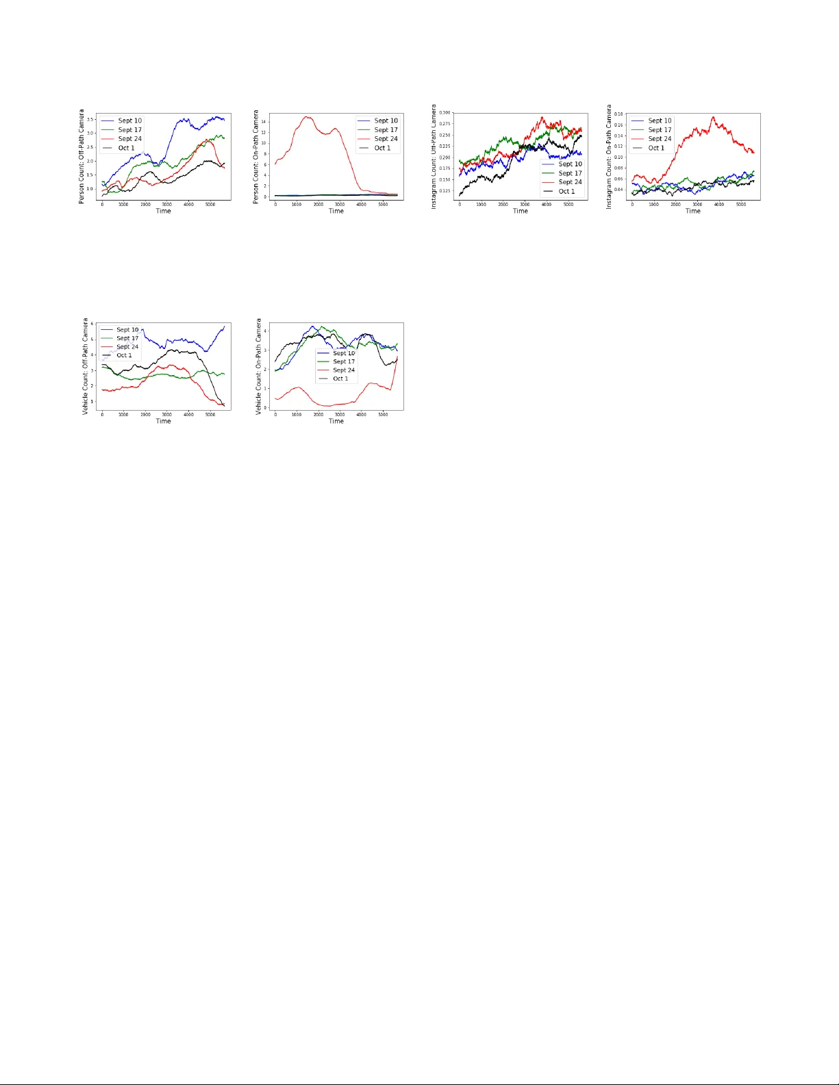
CYCLOST A TION AR Y ST A TISTICAL MODELS AND ALGORITHMS FOR ANOMAL Y DETECTION USING MUL TI-MOD AL D A T A T aposh Banerjee ? Gene Whipps † Prudhvi Gurram †‡ and V ahid T ar okh ± ? School of Engineering and Applied Sciences, Harv ard Uni versity † U.S. Army Research Laboratory ‡ Booz Allen Hamilton ± Department of ECE, Duke Uni versity ABSTRA CT A framew ork is proposed to detect anomalies in multi-modal data. A deep neural network-based object detector is employed to extract counts of objects and sub-ev ents from the data. A cyclostationary model is proposed to model re gular patterns of beha vior in the count sequences. The anomaly detection problem is formulated as a prob- lem of detecting deviations from learned cyclostationary behavior . Sequential algorithms are proposed to detect anomalies using the proposed model. The proposed algorithms are shown to be asymp- totically efficient in a well-defined sense. The dev eloped algorithms are applied to a multi-modal data consisting of CCTV imagery and social media posts to detect a 5K run in New Y ork City . Index T erms — Nonstationary behavior , change detection, deep neural networks, multi-modal data, count data 1. INTRODUCTION Many real-life anomaly detection problems including surveillance, infrastructure monitoring, en vironmental and natural disaster moni- toring, border security using unattended ground sensors, crime hot- spot detection for law enforcement, and real-time traffic monitoring in volve multi-modal data. For example, in a traffic monitoring ap- plication, a decision maker who wishes to detect abnormal behavior or impending congestions, may hav e access to CCTV imagery data, social media data, and other physical sensor data. For such appli- cations, efficient algorithms are needed that can detect anomalies or deviations from normal behavior as quickly as possible. Effecti ve algorithms can be developed only when one has access to, and has a good understanding of, the multi-modal data encountered in these applications. Moti vated by this, in this paper , we develop statistical models and algorithms for detecting anomalous behavior in multi- modal data. The statistical models studied here are moti vated by an analysis of a real-life multi-modal traffic monitoring dataset. The datasets studied in this paper were collected by us around a 5K run that occurred in Ne w Y ork City on Sunday , September 24th, 2017. W e collected data on two Sundays before the run, and one Sunday after the run. W e collected CCTV images and T witter and Instagram posts o ver a geographic re gion from the Red Hook village in Brooklyn on the south end to the Tribeca village on the north end of the collection area. An analysis of the data rev eals that the 5K run changes the av erages of counts of persons and vehicles appearing in the CCTV cameras and the number of Instagram posts per second The work of T aposh Banerjee and V ahid T arokh was supported by a grant from the Army Research Office, W911NF- 15-1-0479. posted in the geographical areas near the run. The counts of per- sons and v ehicles appearing in the CCTV images were obtained by passing the images through a con volution neural network-based ob- ject detector [1], [2], [3], [4]. See Fig. 1. The analysis also suggests that the data has periodic or cyclostationary behavior (see Section 2 for more details). In general, in many monitoring applications, a cer- tain cyclostationary behavior is expected, especially while observing long-term patterns of life, unless an unexpected e vent occurs. COUNTS EVENT)DETECTOR Fig. 1 : Mapping multi-modal data to a sequence of counts In this paper , we define a statistical model to capture the cyclo- stationary behavior . W e also dev elop sequential algorithms to detect deviations aw ay from learned cyclostationary behavior . W e de velop the sequential algorithms in the frame work of quick est change detec- tion [5], [6], [7], and also provide their delay and false alarm analy- sis. The salient features of our paper are as follows. 1. W e use a nov el framew ork introduced by us in [1] for decision making using multi-modal data in volving CCTV images and social media data. In this framework, we use a deep neural network to ex- tract counts of objects from the images. This count is then combined with counts of the number of T weets and Instagram posts near the CCTV cameras. The decision making is then based on the sequence of counts. 2. W e define the concept of an independent and periodically iden- tically distributed (i.p.i.d) process. W e model the count data as an instance of an i.p.i.d. process. W e then propose novel algorithms to detect deviations from learned i.p.i.d. beha vior . See Definition 1. 3. W e define the concept of asymptotic efficienc y for a change point detection algorithm and sho w that our proposed algorithms are asymptotically efficient. See Definition 2. 4. Machine learning and signal processing algorithms for e vent de- tection ha ve been developed in the literature [8], [9], [10], [11], [12], [13], [14] [15]. Ho wev er , in these studies, the abnormal ev ent is of- ten either well-defined and/or can be created to train a model. Since (a) A verage person counts for an off-path camera (b) A verage person counts for an on-path camera Fig. 2 : A verage person counts for the four event days for two cam- eras: one on the path of the event and one outside the path. (a) A verage v ehicle counts for an off-path camera (b) A verage v ehicle counts for an on-path camera Fig. 3 : A v erage vehicle counts for the four event days for two cam- eras: one on the path of the event and one outside the path. the algorithms proposed by us are based on detecting deviations from learned normal behavior , our framework allows for decision mak- ing in rare-e vent scenarios where the anomalous behavior is hard to learn. 2. DA T A ANAL YSIS Details of the data collected, including information on the deep neu- ral network employed, timings and frame rates can be found in our previous work [1]. The objectiv e is to detect the 5K run from the multi-modal data collected. In Figs. 2 to Figs. 4 below , we have plotted av erages of the count data collected on the four days, one ev ent day (Sept. 24), and three non-event day (Sept. 10, Sept. 17, and Oct. 1). The data were extracted in 3-second intervals and av er- aged ov er a sliding window of size 1000. The figures show plots for two selected cameras: one which was a way from the path of the run called the off-path camera, and one which was near the path of the run. The latter is called the on-path camera. In Fig. 2a, we have plotted the av erage person count for the of f- path camera and in Fig. 2b, we ha ve plotted the average person count for the on-path camera. Similar plots for the a verage vehicle counts are sho wn in Fig. 3a and Fig. 3b, and for Instagram counts are shown in Fig. 4a and Fig. 4b. The Instagram counts in Fig. 4 were obtained by averaging the counts for the Instagram posts near the geographi- cal vicinity of the off-path and on-path cameras. W e see a clear in- crease in the av erage count on the ev ent day for the on-path camera. Thus, the 5K run event can be detected using the count sequences from both CCTV data and social media posts. More generally , we can expect counts and sequences of sub-events to capture informa- tion about anomalous beha vior . For example, an event happening twice in a day or two events happening too close to each may indi- cate a deviation from normal beha vior . W e see from the figures that the data is nonstationary in nature, ev en on non-event days. Also, we observe similarity in statistical (a) A verage Instagram post counts for an off-path camera (b) A verage Instagram post counts for an on-path camera Fig. 4 : A verage Instagram post counts for the four event days orig- inating near two CCTV cameras: one on the path of the ev ent and one outside the path. behavior in data across all four days from the off-path camera. W e also see a similarity in behavior in the data from the on-path cam- eras on the non-event days. The data also hav e cyclic behavior . For example, the Instagram count data in Fig. 4a sho w that the data has a trend that repeats itself e very Sunday . Thus, the anomaly detection problem here can be rephrased as either the problem of detecting deviations from normal nonstationary behavior or as the problem of detecting deviations from normal cyclostationary behavior . In [1], we studied a Bayesian problem that captures the problem of detect- ing changes in the levels of nonstationarity . In this paper , we study the latter problem. 3. MA THEMA TICAL MODEL AND PR OBLEM FORMULA TION The central modeling object in this paper is the following. Definition 1. A stochastic pr ocess { Y k } is called independent and periodically identically distributed (i.p.i.d.) if the random variables ar e independent, and ther e is a positive integ er T such that for each i = 1 , · · · , T , the process { Y i + nT } ∞ n =0 is independent and identi- cally distributed (i.i.d). An i.p.i.d. process can be seen as an interleav ed version of T i.i.d. stochastic processes, interleav ed in a round-robin fashion. An i.p.i.d. process is a wide-sense cyclostationary process [16], but has more structure that we will exploit to develop efficient algorithms. W e model a count observation sequence as an i.p.i.d. process. Al- though counts are discrete in nature, the following discussion is v alid for more general random variables as well. In our statistical model, the v ariables { Y k } in the i.p.i.d. process hav e distribution in a parametric family with parameters { θ k } , and the parameter sequence { θ k } is periodic with period T . In other words, we ha ve a sequence model Y k ind ∼ p ( · ; θ k ) , ∀ k , θ k = θ k + T , ∀ k . (1) If the data is collected once per hour , then in the above model, the period T would correspond to T = 24 hours in a day , and the vari- ables Y 1 , · · · , Y T could correspond to the data collected each hour . In many applications, the data is often collected more frequently , at the rate of many samples per second. In such applications, T could be, for example, equal to 24 × 60 × 60 × m , where m is the number of samples collected per second. Note that the statistical model in (1) has only T parameters θ 1 , · · · , θ T . The statistical problem we wish to solve is described as follo ws. Giv en the parameters θ 1 , · · · , θ T , the objectiv e is to observ e the pro- cess { Y k } sequentially over time k and detect any changes in the values of any of the parameters. This change has to be detected in real-time with minimum possible delay , subject to a constraint on the rate of false alarms. The baseline parameters in the problem, the pe- riod T and the parameters within a period θ 1 , · · · , θ T , can be learned from the training data. General tests for learning an i.p.i.d. process will be reported elsewhere. In this paper, we will make additional modeling assumptions to make the learning process simpler . Note that the sequence model (1) studied in this paper is dif fer- ent from the sequence model studied in [17] and [18]. In the model studied in [17] and [18], the random v ariables { Y k − θ k } are mod- eled as Gaussian random variables and the parameters { θ k } are not periodic. Furthermore, the problem there is of simultaneous estima- tion of all the dif ferent parameters { θ k } giv en all the observations { Y k } . That is, the problem is not sequential in nature. It is also not a change point problem. T o summarize, in the absence of an anomaly , we model the data as a nonstationary process. But, we believe there is some regularity in the statistical properties of the process. This allo ws us to model the data as a cyclostationary process. The type of cyclostationary behavior we are interested in is captured by the i.p.i.d. process de- fined abov e. The objective in the anomaly detection problem then is to detect a deviation away from a learned cyclostationary or i.p.i.d. behavior . The algorithm to be used for change detection will depend on the pattern of changes that we assume in the statistical model. W e now discuss two change point models for our problem. As dis- cussed above, if the number of samples taken per second is m and the statistical behavior of the data repeats itself after one week, then we hav e T = 604800 m . In practice, it may be hard to learn a large number of parameters, and detect changes in them. In order to control the complexity of the problem, we assume that the pa- rameters are divided into batches and parameters in each batch are approximately constant. For example, a batch may correspond to data collected in an hour and the average count of objects may not change in an hour . Mathematically , we assume that in each cycle or period of length T , the vector of parameters { θ k } T k =1 is parti- tioned into E batches or episodes. Specifically , for N 0 = 0 and positiv e integers { N e } E e =1 we define B e = { N e − 1 + 1 , · · · , N e } such that { 1 , · · · , T } = ∪ E e =1 B e , B e ∩ B f = ∅ , for e 6 = f . For e ∈ { 1 , · · · , E } , we define θ B e = ( θ N e − 1 +1 , · · · , θ N e ) . Thus, { θ k } T k =1 is partitioned as θ B 1 z }| { θ 1 , · · · , θ N 1 , θ B 2 z }| { θ N 1 +1 , · · · , θ N 2 , · · · , θ B E z }| { θ N E − 1 +1 , · · · , θ N E . (2) Note that we hav e T = P E e =1 | B e | . W e further assume a step model for parameters. Under this as- sumption, the parameters remain constant within a batch resulting in the step-wise constant sequence model θ B 1 z }| { θ (1) , · · · , θ (1) , θ B 2 z }| { θ (2) , · · · , θ (2) , · · · , θ B E z }| { θ ( E ) , · · · , θ ( E ) . (3) That is θ (1) = θ 1 = · · · = θ N 1 , θ (2) = θ N 1 +1 = · · · = θ N 2 , and so on. Thus, if the batch sizes are large, there are only E  T parameters to learn from the data. Also, we hav e | B e | samples for batch e . The objecti ve is then to observe the process { Y k } over time and detect any changes in the parameters θ (1) , · · · , θ ( E ) . W e now define two change point models. Let γ be the change point. If γ = ∞ , i.e., no change occurs, then the stochastic process that we observe, and the parameter v alues, are given by θ B 1 z }| { θ (1) , · · · , θ (1) , θ B 2 z }| { θ (2) , · · · , θ (2) Y 1 , · · · , Y N 1 ,Y N 1 +1 , · · · , Y N 2 , · · · θ B E z }| { θ ( E ) , · · · , θ ( E ) θ B 1 z }| { θ (1) , · · · , θ (1) Y N T − 1 +1 , · · · , Y N T , Y N T +1 , · · · , Y N T +1 . (4) If γ < ∞ , i.e., a change occurs at a finite time γ , we hav e two possible change point models. For k ∈ N , we define the batch of k , b ( k ) , as the v alue j satisfying ( k mod T ) ∈ B j . 1. Change in parameter values in a single batch : In this model, the distribution of the random v ariables { Y k } changes only inside a specific batch say e ∈ { 1 , · · · , E } . That is, in this model, starting at time γ , the parameter values at all the times change as long as the times fall in the batch e . Also, the post-change parameter λ k is different for each k ≥ γ , ev en within a batch. Specifically , if b ( k ) denotes the batch of k then Y k ∼ p ( · ; θ b ( k ) ) , for k < γ ∼ p ( · ; θ b ( k ) ) , for k ≥ γ , b ( k ) 6 = e, ∼ p ( · ; λ k ) , for k ≥ γ , b ( k ) = e, with λ k 6 = θ b ( k ) . (5) The value of e is not known to the decision maker . 2. Change in parameter values in all the batc hes : In this model, the distribution of the random v ariables { Y k } changes for all the batches. Y k ∼ p ( · ; θ b ( k ) ) , for k < γ ∼ p ( · ; λ k ) , for k ≥ γ , with λ k 6 = θ b ( k ) . (6) In a traf fic monitoring scenario, if T corresponds to a day , the single batch change point model may correspond to an anomalous beha vior between 7 am and 8 am everyday , while the all batch change point may correspond to an anomalous behavior throughout the day . W e wish to find a stopping time τ for the sequence { Y k } so as minimize some version of the average of the detection delay τ − γ , with a constraint on the false alarm rate. A popular criterion studied in the literature is that by Pollak [19] min τ sup γ E γ [ τ − γ | τ > γ ] Subj. to E ∞ [ τ ] ≥ β , (7) where E γ denotes expectation with respect to the probability mea- sure when the change occurs at time γ , and β is a given constraint on the mean time to false alarm. Finding optimal solution to such minimax quickest change detection problem is generally hard [5], [6], [7]. W e, therefore, propose algorithms (stopping times), and show that they hav e the follo wing important property , which we also define. Definition 2. A stopping time τ is called asymptotically ef ficient for a change point pr oblem, if as β → ∞ E ∞ [ τ ] ≥ β (1 + o (1)) , and ther e exists a positive constant C such that E 1 [ τ ] ≤ C log β (1 + o (1)) . W e note that most of the classical optimal algorithms in the lit- erature are asymptotically efficient [5], [6], [7], while a trivial al- gorithm like τ ≡ β is not. Furthermore, according to fundamental limit theorems on change point detection [20], the performance of any stopping time cannot be of a smaller order of magnitude than log β (1 + o (1)) . Thus, being asymptotically efficient is an impor- tant property to have for a change detection algorithm. Comments on optimality with respect to the Pollak’ s criterion (7) or Lorden’ s criterion [21] will be provided in an e xtended version of this paper . 4. ALGORITHMS FOR ANOMAL Y DETECTION The change detection model defined in (5) and (6) are similar to change point models studied in sensor network literature [22], [23], [24], where a change can affect one, or all the sensors. Observ a- tions from a batch can be viewed as observations from a sensor . The important difference between our problem and the sensor net- work problem is that the decision maker here observ es the data from batches in sequence, i.e., does not have access to all the data at the same time. Nonetheless, the analogy between the two problems pro- vides us with guidelines for identifying relev ant algorithms for our problem. W e will make some assumptions about the w ay change oc- curs to simplify our notations, algorithms, and analysis. Algorithms for more general change point models can be developed by follo wing the techniques discussed below . 4.1. Algorithm for Detecting Change in a Single Batch W e assume that after the change occurs in a single batch e , the post- change parameter λ k is the same for all the variables in the batch e . Since it is not known in which batch e the change occurs, we ex ecute E algorithms, one for each batch, and raise an alarm as soon as any of the algorithms detect the change. Mathematically , define the following statistics for data from batch e : W e n = max 1 ≤ k ≤ n sup λ ∈ Λ e n X i = k : b ( i )= e log[ p ( Y i ; λ ) /p ( Y i ; θ ( e ) )] , (8) where Λ e = { λ : | λ − θ ( e ) | ≥  } . (9) Also, define τ e as the stopping time for the batch e : τ e = inf { n ≥ 1 : W e n > A } . (10) Here,  > 0 is the minimum amount of change from the baseline parameter θ ( e ) the algorithm can detect. Note that the condition i = k : b ( i ) = e ensures that only data from the batch e are utilized for computing the statistic W e n . Our change detection algorithm is the minimum of these stopping times. τ o = min 1 ≤ e ≤ E τ e . (11) Theorem 4.1. Suppose the post-change parameter space Λ e in (9) is finite. Then, the stopping time τ o in (11) is asymptotically efficient. Pr oof. The false alarm result is true because τ e stochastically dom- inates Lorden’ s stopping time designed for pre-change parameter θ ( e ) . The finite family assumption and martingale arguments im- ply setting A = log β (1 + o (1)) will ensure E ∞ [ τ o ] ≥ β (1 + o (1)) , as β → ∞ [22] . For delay , it can be shown that if λ is the true post-change parameter in batch e then as β → ∞ , E 1 [ τ o ] ≤ log( β )(1+ o (1)) I ( λ ) κ , where κ = (1 + P f 6 = e | B f | / | B e | ) , and I ( λ ) is the Kullback-Leibler diver gence between p ( · , λ ) and p ( · , θ ( e ) ) , imply- ing asymptotic efficienc y .  (a) T est statistic W n for the on-path camera. (b) W n for Instagram replotted. Fig. 5 : Plots of test statistic W n from (12). 4.2. Algorithm for Detecting Change in All the Batches W e assume that after the change occurs, the post-change parame- ter λ k is the same for all the v ariables in a batch e . Since the change occurs in all the batches, we use an algorithm that combines observa- tions from all the batches. Mathematically , we compute the statistic W n = max 1 ≤ k ≤ n sup λ ( e ) ∈ Λ ( e ) , e ≤ E n X i = k log[ p ( Y i ; λ ( b ( i )) ) /p ( Y i ; θ ( b ( i )) )] , (12) and declare an anomaly at the stopping time τ a = inf { n ≥ 1 : W n > A } . (13) Theorem 4.2. Suppose the post-change parameter space Λ e in (9) is finite. Then, the stopping time τ a in (13) is asymptotically efficient. Pr oof. Independence and separation of suprema over λ ( e ) giv es W n ≤ P E e =1 W e n . The false alarm result follows from the pre vious theorem because { P E e =1 W e n > A } im- plies { max E e =1 W e n > A/E } . For the delay analysis, note that removing the maximum operators gives W n ≥ P E e =1 P n i =1: b ( i )= e log[ p ( Y i ; λ ( e ) ) /p ( Y i ; θ ( e ) )] . Asymptotic ef fi- ciency follows because the latter’ s behavior is similar to that of a random walk and based on the ar guments in [26].  5. NUMERICAL RESUL TS AND CONCLUSIONS W e now apply the dev eloped algorithm to the NYC data. Due to a paucity of space, the performance of the algorithm for simulated data will be reported elsewhere. W e apply τ a to the count data be- cause the change appears to affect the entire day’ s data. In Fig. 5a, we hav e plotted the e volution of the test statistic W n for all the count data: person count, vehicle count, and the Instagram count. In the figure, the data for each modality is arranged in a concatenated fash- ion, with labeled segments separated via red vertical lines. Each day has 6598 samples. T o compute the statistic, we di vided the data into four batches, with the first three batches being of length 1500 . W e modeled the data as a sequence of Poisson random variables. W e used the count data from Sept. 10 (one of the non-event days) to learn the averages of these Poisson random variables for each of the four batches. W e assumed that there is only one post-change param- eter per batch that is equal to twice the normal parameter (half the normal parameters for vehicles) for that batch. W e then applied the test to all the four days of data. In Fig. 5b, we hav e replotted the test statistic applied to the Instagram counts. As seen from the figures, the algorithm detects the anomaly that occurs on Sept. 24 (ev ent day). In future, we will apply the algorithms to other multi-modal datasets to test their effecti veness. W e will also study optimality of the proposed algorithms for Lorden’ s and Pollak’ s criteria. 6. REFERENCES [1] T . Banerjee, G. Whipps, P . Gurram, and V . T arokh, “Sequen- tial e vent detection using multimodal data in nonstationary en- vironments, ” in Pr oc. of the 21st International Conference on Information Fusion , July 2018. [2] S. Ren, K. He, R. B. Girshick, and J. Sun, “Faster R-CNN: tow ards real-time object detection with region proposal net- works, ” CoRR , v ol. abs/1506.01497, 2015. [3] K. Simonyan and A. Zisserman, “V ery deep conv olu- tional networks for large-scale image recognition, ” CoRR , vol. abs/1409.1556, 2014. [4] M. Everingham, L. V an Gool, C. K. I. Williams, J. Winn, and A. Zisserman, “The pascal visual object classes (voc) chal- lenge, ” International Journal of Computer V ision , vol. 88, pp. 303–338, June 2010. [5] V . V . V eeravalli and T . Banerjee, Quickest Change Detec- tion . Academic Press Library in Signal Processing: V olume 3 – Array and Statistical Signal Processing, 2014. http: //arxiv.org/abs/1210.5552 . [6] H. V . Poor and O. Hadjiliadis, Quickest detection . Cambridge Univ ersity Press, 2009. [7] A. G. T artako vsky , I. V . Nikiforov , and M. Basseville, Sequen- tial Analysis: Hypothesis T esting and Chang e-P oint Detection . Statistics, CRC Press, 2014. [8] R. Panda and A. K. Roy-Chowdhury , “Multi-vie w surveil- lance video summarization via joint embedding and sparse op- timization, ” IEEE T ransactions on Multimedia , vol. 19, no. 9, pp. 2010–2021, 2017. [9] S. C. Lee and R. Nev atia, “Hierarchical abnormal ev ent de- tection by real time and semi-real time multi-tasking video surveillance system, ” Machine vision and applications , v ol. 25, no. 1, pp. 133–143, 2014. [10] R. Szechtman, M. Kress, K. Lin, and D. Cfir , “Models of sen- sor operations for border surveillance, ” Naval Resear ch Logis- tics (NRL) , vol. 55, no. 1, pp. 27–41, 2008. [11] D. B. Neill and W . L. Gorr, “Detecting and preventing emerg- ing epidemics of crime, ” Advances in Disease Surveillance , vol. 4, no. 13, 2007. [12] R. Mitchell and I. R. Chen, “Effect of intrusion detection and response on reliability of cyber physical systems, ” IEEE T rans- actions on Reliability , vol. 62, pp. 199–210, March 2013. [13] E. D’Andrea, P . Ducange, B. Lazzerini, and F . Marcelloni, “Real-time detection of traffic from T witter stream analy- sis, ” IEEE T ransactions on Intelligent T r ansportation Systems , vol. 16, pp. 2269–2283, Aug 2015. [14] E. W . Dereszynski and T . G. Dietterich, “Probabilistic models for anomaly detection in remote sensor data streams, ” arXiv pr eprint arXiv:1206.5250 , 2012. [15] T . Sakaki, M. Okazaki, and Y . Matsuo, “Earthquake shakes T witter users: Real-time e vent detection by social sensors, ” in Pr oceedings of the 19th Int. Conf. on W orld W ide W eb , pp. 851–860, A CM, 2010. [16] W . A. Gardner, A. Napolitano, and L. Paura, “Cyclostation- arity: Half a century of research, ” Signal pr ocessing , vol. 86, no. 4, pp. 639–697, 2006. [17] I. M. Johnstone, Gaussian estimation: Sequence and wavelet models . Book Draft, 2017. A vailable for down- load from http://statweb.stanford.edu/ ˜ imj/ GE_08_09_17.pdf . [18] A. B. Tsybakov , Introduction to nonparametric estimation . Springer Series in Statistics. Springer , New Y ork, 2009. [19] M. Pollak, “Optimal detection of a change in distribution, ” Ann. Statist. , vol. 13, pp. 206–227, Mar . 1985. [20] T . L. Lai, “Information bounds and quick detection of param- eter changes in stochastic systems, ” IEEE T rans. Inf. Theory , vol. 44, pp. 2917 –2929, No v . 1998. [21] G. Lorden, “Procedures for reacting to a change in distribu- tion, ” Ann. Math. Statist. , vol. 42, pp. 1897–1908, Dec. 1971. [22] A. G. T artakovsk y and V . V . V eeravalli, “ An efficient sequen- tial procedure for detecting changes in multichannel and dis- tributed systems, ” in IEEE International Confer ence on Infor- mation Fusion , vol. 1, (Annapolis, MD), pp. 41–48, July 2002. [23] Y . Mei, “Ef ficient scalable schemes for monitoring a large number of data streams, ” Biometrika , vol. 97, pp. 419–433, Apr . 2010. [24] A. G. T artakovsk y and V . V . V eeravalli, “ Asymptotically opti- mal quickest change detection in distributed sensor systems, ” Sequential Analysis , vol. 27, pp. 441–475, Oct. 2008. [25] T . Banerjee, H. Firouzi, and A. O. Hero III, “Quickest detection for changes in maximal knn coherence of random matrices, ” arXiv pr eprint arXiv:1508.04720 , 2015. [26] M. W oodroofe, Nonlinear Renewal Theory in Sequential Anal- ysis . CBMS-NSF regional conference series in applied mathe- matics, SIAM, 1982.