Falsification of Cyber-Physical Systems Using Deep Reinforcement Learning

With the rapid development of software and distributed computing, Cyber-Physical Systems (CPS) are widely adopted in many application areas, e.g., smart grid, autonomous automobile. It is difficult to detect defects in CPS models due to the complexities involved in the software and physical systems. To find defects in CPS models efficiently, robustness guided falsification of CPS is introduced. Existing methods use several optimization techniques to generate counterexamples, which falsify the given properties of a CPS. However those methods may require a large number of simulation runs to find the counterexample and is far from practical. In this work, we explore state-of-the-art Deep Reinforcement Learning (DRL) techniques to reduce the number of simulation runs required to find such counterexamples. We report our method and the preliminary evaluation results.

💡 Research Summary

The paper addresses the challenge of efficiently finding counterexamples for safety‑critical cyber‑physical systems (CPS) by integrating deep reinforcement learning (DRL) into robustness‑guided falsification. Traditional falsification techniques, such as simulated annealing (SA) and cross‑entropy (CE), treat the input signal as a whole and optimize it using global stochastic search. While these methods can eventually locate inputs that violate a Signal Temporal Logic (STL) specification, they typically require thousands of expensive simulation runs, making them impractical for complex CPS models.

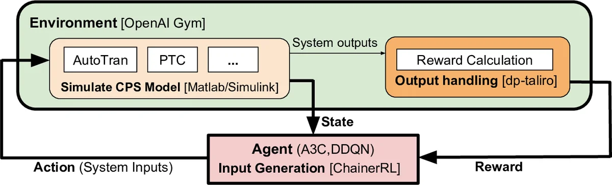
To overcome this limitation, the authors reformulate falsification as a reinforcement‑learning problem. An agent interacts with the CPS model in discrete time steps of size ΔT, generating a piecewise‑constant input at each step. After each action the simulator (implemented in MATLAB/Simulink and wrapped by an OpenAI Gym environment) returns the new system state (output variables). The agent receives a reward that reflects the STL robustness of the current trajectory:

 r_i = exp(−ρ(ϕ, x_i, t_i)) − 1

where ρ(ϕ, x, t) is the quantitative robustness of the sub‑formula ϕ at time t. This reward is maximal when the robustness is low (i.e., the property is close to being violated), encouraging the agent to drive the system toward falsification. The discount factor γ is set to 1, so the cumulative reward directly mirrors the robustness trend over the episode.

Two state‑of‑the‑art DRL algorithms are employed:

1. Asynchronous Advantage Actor‑Critic (A3C) – a policy‑gradient method that runs multiple parallel workers, each collecting experience and updating a shared network asynchronously. This yields fast exploration and stable learning without the need for experience replay.

2. Double Deep Q‑Network (DDQN) – a value‑based method that mitigates overestimation of Q‑values by decoupling action selection and evaluation. It uses a target network and experience replay to stabilize learning.

Both algorithms are used out‑of‑the‑box via the ChainerRL library, with default hyper‑parameters, to demonstrate that the approach does not rely on extensive tuning.

The experimental platform is the well‑known automatic transmission (AT) benchmark, a hybrid model with throttle and brake as inputs and vehicle speed (v), engine angular speed (ω), and gear state (g) as outputs. Nine STL properties are examined: six derived from the original AT benchmark (ϕ₁–ϕ₆) and three newly crafted specifications (ϕ₇–ϕ₉). Each property is expressed as a “life‑long” formula □ϕ, which the authors convert to a past‑dependent form to simplify reward computation. For every property, 20 independent falsification runs are performed, each allowed up to 200 episodes. The number of episodes required to achieve falsification (or 200 if unsuccessful) and the success rate are recorded.

Key findings:

• Higher success rates – RL‑based methods achieve success rates between 65 % and 100 % across all properties, whereas SA and CE often fall below 70 % and sometimes fail entirely (e.g., ϕ₇ with SA).
• Fewer episodes – For five of the nine properties (ϕ₁, ϕ₂, ϕ₆, ϕ₇, ϕ₉) A3C or DDQN require markedly fewer episodes than the baselines (median reductions from >100 episodes to <20). Statistical significance is confirmed by Fisher’s exact test (p < 0.05) and Mann‑Whitney U‑test (p < 0.001).
• Algorithmic nuances – DDQN tends to output extreme action values, which harms performance on properties involving discrete variables (ϕ₃, ϕ₄). A3C, being policy‑based, handles continuous action spaces more gracefully.
• ΔT sensitivity – The discretization step ΔT influences all methods; the authors report the best ΔT for each algorithm/property (typically 1, 5, or 10).

The architecture integrates three components: (i) input generation via DRL (ChainerRL), (ii) simulation of the CPS model (MATLAB/Simulink wrapped as a Gym environment), and (iii) robustness evaluation and reward calculation (dp‑Taliro). This modular design allows swapping any component (e.g., using a different simulator or a more advanced RL library) without redesigning the whole pipeline.

In conclusion, the study demonstrates that casting robustness‑guided falsification as a reinforcement‑learning problem can substantially reduce the number of costly simulations needed to discover counterexamples. The reward formulation directly ties STL robustness to RL objectives, enabling the agent to learn a policy that steers the system toward unsafe regions efficiently. The authors acknowledge limitations, such as the need for better handling of discrete action spaces and the reliance on a single benchmark. Future work is planned to explore additional DRL algorithms (e.g., PPO, SAC), extend evaluations to larger CPS domains (power grids, robotics), and investigate multi‑agent or hierarchical strategies for even more complex specifications.