Physics-informed Machine Learning Method for Forecasting and Uncertainty Quantification of Partially Observed and Unobserved States in Power Grids

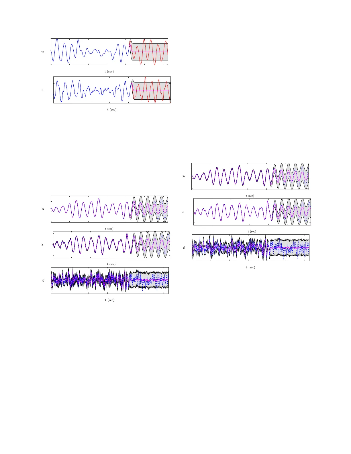
Physics-inf ormed Machine Learning Method f or F orecasting and Uncertainty Quantification of Partially Obser ved and Unobser ved States in P ower Grids Ramakrishna T ipireddy Pacific Northwest National Laboratory Ramakrishna.T ipireddy@pnnl.gov Alexandre T artakovsk y Pacific Northwest National Laboratory Alexandre.T artakovsk y@pnnl.gov Abstract W e pr esent a physics-informed Gaussian Pr ocess Re gression (GPR) model to pr edict the phase angle, angular speed, and wind mechanical power fr om a limited number of measurements. In the traditional data-driven GPR method, the form of the Gaussian Pr ocess covariance matrix is assumed and its parameters ar e found fr om measur ements. In the physics-informed GPR, we tr eat unknown variables (including wind speed and mechanical power) as a random pr ocess and compute the covariance matrix fr om the resulting stoc hastic power grid equations. W e demonstrate that the physics-informed GPR method is significantly mor e accurate than the standar d data-driven one for immediate for ecasting of generator s’ angular velocity and phase angle . W e also show that the physics-informed GPR pr ovides accurate pr edictions of the unobserved wind mechanical power , phase angle, or angular velocity when measurements fr om only one of these variables ar e available. The immediate for ecast of observed variables and pr edictions of unobserved variables can be used for effectively managing power grids (electricity market clearing, re gulation actions) and early detection of abnormal behavior and faults. The physics-based GPR for ecast time horizon depends on the combination of input (wind power , load, etc.) corr elation time and char acteristic (r elaxation) time of the power grid and can be extended to short and medium-r ange times. 1. Introduction Real-time monitoring and immediate forecasting of the power grid dynamics is important for efficient operation of the po wer grid, including electricity mark et clearing and regulation actions [1]. Other applications that require forecasting include early detection of faults and instabilities and the effecti ve operation of controllers. Despite the fact that modern power grids are heavily instrumented, directly measuring all po wer grid states remains impractical. Inherent high-frequenc y oscillations of the power grid dynamics, compounded by increasing penetration of rene wable ener gy sources, make immediate forecasting very challenging. Here, we present a “physics-informed” Gaussian Process Regression (GPR) method for monitoring (computing unobserved states) and immediate forecasting of po wer grid dynamics from measurements of (observed) states. W e demonstrate that when partial (past) observations of variables are a vailable, the proposed physics-informed GPR is significantly more accurate for forecasting than the standard “data-dri ven” GPR. When observations of the variables (states) of interest are not av ailable, the physics-informed GPR still can provide equally good predictions based on measurements of other states, while the data-dri ven GPR becomes inapplicable. Short-term forecasting in power grids has been addressed with various methods, including machine learning (support vector machines [2], Deep Neural Networks [3, 4, 5]) and statistical (e.g., the autoregressi ve integrated moving average method [6]) methods. GPR [7], another machine learning method, has been used for forecasting observ ed states with the model hyperparameters learned from measurements [8, 9]. In this work, we refer to this standard GRP method as the “data-dri ven” GPR. Challenges with the data-driv en GPR include: 1) it requires a large amount of data collected at high frequency (relativ e to the process’ correlation time), 2) the estimation of hyperparameters can be affected by the noise in measurements, and 3) it cannot predict unobserved states. Unlike some engineered and natural systems, power grid dynamics is well understood, and equations gov erning power grid dynamics have solid theoretical foundations. Using this characteristic of power grids, we propose a nov el physics-informed GPR approach with the cov ariance matrix computed as a solution of stochastic power grid equations. W e consider a grid with wind-po wered generators. Because wind mechanical power is oscillating in time and deterministically unknown, it must be modeled as a correlated-in-time random process to properly describe the effect of wind fluctuations on the power grid dynamics and small signal and transient stability [10]. Random mechanical wind po wer transforms power grid equations into stochastic equations [11, 12]. T o compute the cov ariance matrix, we solve stochastic power grid equation using the strong stability preserving Runge-Kutta (RK) scheme for different realizations of mechanical wind power [13, 12]. 2. Problem description T o introduce the physics-informed GPR approach, we consider a power system with a single wind-po wered generator and infinite bus, described by the swing equations [14, 11]: dθ dt = ω B ( ω − ω S ) , dω dt = ω S 2 H [ P m − P e − D ( ω − ω S )] , (1) subject to the initial conditions θ ( t = 0) = θ 0 and ω ( t = 0) = ω 0 . Here, θ ∈ [0 , 2 π ) is the phase angle between the axis of the generator and the magnetic field, ω ∈ ( −∞ , ∞ ) is the angular generator speed, H is the generator inertia, ω B is the base speed, ω s is the synchronization speed, and P e is the electric power supplied by the generator to the infinite bus and is related to the phase angle θ as P e = P max sin θ, (2) where P max = E V X , E is the internal energy , V is the bus voltage, and X is the total reactance in the system. The mechanical power of wind, P m ( t ) = h P m ( t ) i + P 0 m ( t ) , is modeled as a stochastic process with mean h P m i > 0 , zero-mean fluctuations h P 0 m i = 0 , v ariance σ 2 , and the cov ariance function h P 0 m ( t ) P 0 m ( s ) i = σ 2 exp  − | t − s | λ  , (3) where λ is the correlation time. T o solve the gov erning equations, we model P 0 m ( t ) as an Ornstein-Uhlenbeck (O-U) process, satisfying the stochastic ordinary differential equation (ODE) [13]: dP 0 m = − 1 λ P 0 m dt + r 2 λ σ dW , (4) subject to the initial condition P 0 m (0) = P 0 m, 0 , (5) where W is the standard W iener process. The resulting equations are solved using a second-order strong stability preserving RK scheme [13] (described in Section 3). The initial condition P 0 m, 0 ( t ) is obtained from the stationary Gaussian distribution with zero mean and v ariance σ 2 . The initial conditions for θ and ω are set to θ 0 = arcsin h P m i P max and ω 0 = ω S . 3. Strong stability pr eserving Runge-Kutta scheme T o introduce the RK scheme, we define the vector y = [ θ , ω ] T and scalar z = P 0 m functions of time and rewrite the go verning equations as dy = f ( y ) dt + g ( y ) z dt, dz = − az dt + bdW, (6) where f ( y ) =  ω B ( ω − ω S ) dt ω S 2 H [ h P m i − P max sin θ − D ( ω − ω S )]  , g ( y ) =  0 ω S 2 H P 0 m  , a = 1 λ , and b = q 2 λ σ. The RK discretization of Eq (6) is [13]: y k +1 = y k + h 2 { ( f + g z ) k + ( f + g z ) ¯ k } + 1 √ 12 g k bh 3 / 2 η k , z k +1 = z k + bξ k h 1 / 2 + h 2 a ( z k + z ¯ k ) + 1 √ 12 abh 3 / 2 η k , (7) where h is the time step, ξ k and η k are the realizations of independent standard Gaussian random variables ξ and η at time step k , f ¯ k = f ( y ¯ k ) , g ¯ k = g ( y ¯ k ) , y ¯ k = y k + ( f + g z ) k h , and z ¯ k = z k + bξ k h 1 / 2 + az k h. 4. Gaussian Process Regr ession model GPR giv es an unbiased estimate of variable x f = [ x f 1 , ..., x f N f ] T ( x f i = x f ( t i ) ) at different times t i and associated uncertainty giv en observ ations x o = [ x o 1 , ..., x o N o ] T ( x o i = x o ( ˜ t i ) ). Here, x o and x f can represent the same power grid states, where, for example, x o is the observed ω , x f is the forecasted ω , and t N o < ˜ t 1 . Alternativ ely , x o and x f could be different states, e.g., x o is observed ω , and x f is predicted θ at the same times when ω is observed (i.e., t i = ˜ t i ) or at different times. Let define x = [ x o , x f ] T . Next, we assume that x is the Gaussian process with  x o x f  ∼ N  ¯ x o ¯ x f  ,  C oo C of C f o C f f  , (8) where ¯ x o and ¯ x f are the so-called prior (or , unconditional) mean of x o and x f , respectively , and C oo , C of , C f o , and C f f are the respectiv e prior cov ariances between x o and x o , x o and x f , x f and x o , and x f and x f . Then, GPR defines the conditional (or posterior) estimate of x f giv en x o as ˆ x f ( t ) = C f o C − 1 oo x o (9) and the conditional cov ariance as ˆ C f f = C f f − C f o C − 1 oo C of . (10) The main challenge in GPR is to obtain prior statistics, i.e., prior mean and cov ariance functions. In the standard data-driv en GPR method, prior statistics is found from measurements of x o and x f using the so-called marginal lik elihood [8, 9]. Usually , a form of the cov ariance function is assumed, and the parameters (variance and correlation length) are found by minimizing the negati ve marginal likelihood of the Gaussian process. Such a purely data-driv en approach is impossible to implement for reconstructing unobserved states from observed states without making assumptions about the correlation between unobserved and observed states. Our proposed physics-informed GPR approach combines GPR and power grid equations. Specifically , we use Eqs (1) and (5) to compute the mean and cov ariance functions in Eq (8). Let ω ( n ) k , θ ( n ) k , and P 0 ( n ) m,k k = 0 , 1 , ..., K be numerical solutions of Eqs (1) and (5) at time t k with the initial condition P 0 ( n ) m, 0 ( n = 0 , 1 , 2 , · · · , N ) drawn from the Gaussian distribution. Then, the mean and cov ariance of the state x ( n ) k ( x = ω , θ , P 0 m ) are computed respecti vely as ¯ x ( t k ) = ¯ x k = 1 N N X n =1 x n k , k = 1 , · · · , K (11) and C xx ( t j , t k ) = 1 N − 1 N X n =1 ( x n j − ¯ x j )( x n k − ¯ x k ) , j, k = 1 , · · · , K . (12) The cov ariance between different variables (e.g., between ω and θ ) is computed as: C ω θ ( t j , t k ) = 1 N − 1 N X n =1 ( ω n j − ¯ ω j )( θ n k − ¯ θ k ) , j, k = 1 , · · · , K . (13) 5. Numerical results 0 5 10 15 20 25 0 0.5 1 0 5 10 15 20 25 0.99 1 1.01 0 5 10 15 20 25 -1 0 1 Figure 1. One realization of θ ( t ) , ω ( t ) , and P 0 m ( t ) . The numerical solutions are obtained with P max = 2 . 1 p.u., H = 5 s, D = 5 p.u., h P m i = 0 . 9 p.u., ω B = 120 π rad/s, λ = 0 . 026 s, and ω S = 1 . 0 . The solutions are computed for a total time of T = 25 s with a time step h = 0 . 0025 s. The initial conditions are assumed to be θ 0 = 0 . 45 , ω 0 = 1 . 0 . One thousand Monte Carlo realizations are performed with P 0 ( n ) m, 0 = ξ n , ( n = 0 , 1 , ..., 999 ), where ξ n is a Gaussian random variable with zero mean and v ariance σ = 0 . 1 . Figure 2. 50 realizations of θ ( t ) and ω ( t ) . Fig. 1 shows one realization of θ ( t ) , ω ( t ) , and P 0 m ( t ) . It illustrates that θ and ω have higher-frequenc y oscillations on the scale of 1 s caused by the high-frequency oscillations in P 0 m and lower -frequency oscillations on the scale of 10 s that are proportional to the relaxation time of the system H ω s D . In this work, we focus on modeling higher-frequency dynamics. Fig. 2 sho ws 50 realizations of θ ( t ) and ω ( t ) . Mean and standard de viation of θ and ω approach asymptotic values after approximately 20 s, which are shown in Figs. 3 and 4. W e consider three different cases for time series forecasting. In the first case, we assume that partial measurements of θ and ω up to a certain time are av ailable and forecast of θ and ω beyond this time using 0 5 10 15 20 25 0.35 0.4 0.45 0.5 0.55 0 5 10 15 20 25 0.998 0.999 1 1.001 1.002 Figure 3. Mean of θ and ω . 0 5 10 15 20 25 0 0.05 0.1 0.15 0 5 10 15 20 25 0 0.5 1 1.5 2 2.5 10 -3 Figure 4. Standard deviation of θ and ω . conditional estimation of mean and standard deviation from the Gaussian process model. In the second case, we assume that partial measurements are available only for θ and predict θ , ω , and P 0 m . In the third case, we predict θ , ω , and P 0 m when only partial ω measurements are av ailable. 5.1. Case 1: F orecast of θ and ω giv en past measurements of θ and ω 0 2 4 6 8 10 12 0.3 0.4 0.5 0.6 0 2 4 6 8 10 12 0.995 1 1.005 Figure 5. Fo recast for θ and ω (magenta line) and the erro r b ounds (gray area) corresponding to tw o standa rd deviations of θ and ω , respectively . The blue dashed line sho ws the ground truth (realization one). In this case, we assume that the θ ( t ) and ω ( t ) measurements are av ailable until time t = 8 . 3375 s ev ery 0.0025 s. Our objectiv e is to forecast θ ( t ) and ω ( t ) for times greater than 8 . 3375 s. T o test our approach, we compute prior statistics as described in Section 4 and use two randomly selected solutions of the governing equations as ground truth. Specifically , we treat the solution for t < 8 . 3375 s as observations of θ ( t ) and ω ( t ) and use these observ ations as input for the GRP model to predict θ ( t ) and ω ( t ) for t > 8 . 3375 s. The second part of the solutions is used to validate the GPR predictions. For these two synthetic observ ation sets, Figs. 5 and 6 show the forecast (mean values) of θ and ω (magenta line) and uncertainty , represented by the gray area corresponding to two standard deviations of θ and ω . The blue dashed line sho ws the ground truth. In both cases, the physics-informed GPR method is able to provide an accurate deterministic forecast of θ and ω for the time horizon of at least 2 s or 50 λ , i.e., the mean prediction of the GPR closely agrees with the ground truth for at least 20 λ , after which the mean prediction quality deteriorates. More importantly , the “statistical forecast” is accurate for at least 4 s or 80 λ , i.e., the ground truth lies within the predicted uncertainty en velope. 0 2 4 6 8 10 12 0.2 0.4 0.6 0 2 4 6 8 10 12 0.995 1 1.005 Figure 6. Fo recast for θ and ω (magenta line) and the erro r b ounds (gray area) corresponding to tw o standa rd deviations of θ and ω , respectively . The blue dashed line sho ws the ground truth (realization t wo). For comparison, we also forecast θ and ω using the standard data-dri ven GRP method with the cov ariance obtained from the marginal likelihood method (Fig. 7). The comparison of the two methods demonstrates that the the physics-informed GPR performs much better than the data-driven GPR. The data-dri ven GPR provides an accurate mean prediction for less than 5 λ and statistical prediction for less than 20 λ . 0 2 4 6 8 10 12 0.3 0.4 0.5 0 2 4 6 8 10 12 0.998 1 1.002 Figure 7. Fo recast for θ and ω (magenta line) and the erro r b ounds (gray area) corresponding to tw o standa rd deviations of θ and ω , respectively , computed using the standa rd data-driven GPR with cova riance obtained from the marginal lik eliho o d metho d. Red line shows the ground truth. 5.2. Case 2: F orecast θ , ω , and P 0 m given measurements of θ 0 2 4 6 8 10 12 0.2 0.4 0.6 0 2 4 6 8 10 12 0.995 1 1.005 0 2 4 6 8 10 12 -0.2 0 0.2 Figure 8. Fo recast of θ , ω , and P 0 m with no observations of θ for t > 8 . 3375 . In this case, we assume that θ ( t ) measurements are av ailable for t < 8 . 3375 s ev ery 0.0025 s. Our goal is to predict θ ( t ) for t > 8 . 3375 and ω ( t ) and P 0 m ( t ) for the entire time interval t ∈ [0 , 12 . 5] s. As in Case 1, we compute prior statistics by solving the stochastic power grid equations and use a randomly selected solution as observations of θ ( t ) for t < 8 . 3375 s and ground truth to validate the physics-informed GPR predictions of θ ( t ) (for t > 8 . 3375 ), ω ( t ) , and P 0 m ( t ) . Fig. 8 shows the predictions of θ , ω , and P 0 m and the ground truth results. Notably , the forecast of ω is exactly the same as in Case 1 (Fig 6) because the ω observations are the same in these two cases. The prediction for θ ( t ) is excellent for t < 8 . 3375 when ω ( t ) measurements are av ailable. This is e vident by the mean prediction being very close to the ground truth and very small standard deviation (i.e., the narro w gray “uncertainty” area). For t > 8 . 3375 , the agreement between mean prediction and ground truth is almost as good as in Case 1. Also, as in Case 1, the ground truth remains within the uncertainty en velope. Similar results are observed for P m . These results demonstrate that the physics-informed GPR is very accurate for computing unobserved v ariables. This is important because some variables, including P m , are difficult to measure directly . 5.3. Case 3: F orecast of θ , ω , and P 0 m given measurements of ω 0 2 4 6 8 10 12 0.2 0.4 0.6 0 2 4 6 8 10 12 0.995 1 1.005 0 2 4 6 8 10 12 -0.2 0 0.2 Figure 9. Fo recast of θ , ω , and P 0 m p ro cess with no observations of ω for t > 8 . 3375 . This case is similar to Case 2, except instead of θ ( t ) measurements, we hav e ω ( t ) measurements for t < 8 . 3375 . Our objectiv e is to predict ω ( t ) for t > 8 . 3375 and θ ( t ) and P 0 m ( t ) for the entire time interval t ∈ [0 , 12 . 5] s. Fig. 9 presents measurements of ω and predicted ω ( t ) , θ ( t ) , and P 0 m ( t ) , as well as the ground truth solutions for these variables. As in Case 2, physics-informed GPR provides excellent predictions of θ ( t ) and P 0 m ( t ) for t < 8 . 3375 and a similarly good prediction for t > 8 . 3375 s as in Case 1 where the θ ( t ) measurements for t < 8 . 3375 are a vailable. Next, we assume that 333 ω ( t ) measurements (shown by red circles in Fig. 10) are av ailable for t > 8 . 3375 . Fig. 10 shows that these measurements significantly improv e prediction of the (unobserved) θ ( t ) and P 0 m ( t ) v ariables. 0 2 4 6 8 10 12 0.3 0.4 0.5 0.6 0 2 4 6 8 10 12 0.996 0.998 1 1.002 1.004 0 2 4 6 8 10 12 -0.2 0 0.2 Figure 10. Fo recast of θ , ω , and P 0 m with 333 observations of ω for t > 8 . 3375 . Fig. 11 depicts a comparison of the physics-informed GPR prediction of P 0 m based on measurements of θ and ω . This comparison reveals that the predictions of P 0 m ( t ) are reasonably good in both cases and better when θ measurements are av ailable instead of ω measurements. This shows that θ is correlated more strongly with P 0 m than ω . 0 2 4 6 8 10 12 -0.2 0 0.2 0 2 4 6 8 10 12 -0.2 0 0.2 Figure 11. Fo recast of P 0 m p ro cess when observations of a) θ and b) ω are available. 6. Discussion and conclusions W e hav e presented a physics-informed Gaussian Process Regression (GPR) model to predict the phase angle, angular speed, and wind mechanical power when past measurements of all or some of these states are av ailable. In the traditional data-dri ven GPR method, a form of the cov ariance matrix of the Gaussian Process model is first assumed and then its parameters are found from measurements. In the physics-informed GPR, we treat unknown variables, including wind speed and mechanical power , as a random process and compute the cov ariance matrix of the GPR model from the resulting stochastic power grid equations. W e ha ve demonstrated that the physics-informed GPR method is significantly more accurate than the standard data-driv en GPR method for forecasting generators’ angular velocity and phase angle. W e also have shown that the physics-informed GPR provides accurate predictions of the unobserved wind mechanical power , phase angle, or angular velocity when measurements of only one of these variables are a vailable. One advantage of GPR over neural-network-based methods is that its predictions come with uncertainty bounds, i.e., GPR predicts the mean value and standard deviation of quantities of interest. W e hav e demonstrated that the ph ysics-informed GPR accurately and reliably (with small uncertainty) predicts unobserved v ariables from observed ones for the entire time interval where observ ations of other (correlated) variables are available. For forecasting, the uncertainty in predicted values slowly increases with the time horizon. In the considered cases, the forecasted mean values were accurate in the time horizon equal to as man y as 200 correlation times of the wind power fluctuations. For larger time horizons, we hav e noted the predicted values to be within two standard deviations from the ground truth. In this study , we hav e modeled high-frequency power grid dynamics produced by high-frequency wind oscillations. The correlation length of the wind mechanical power in the simulated data was λ = 0 . 026 s, and the accurate mean values were obtained for up to 2 s time horizon. Such high-frequenc y oscillations hav e been shown to have a significant effect on small signal stability [10, 11, 12]. For economic load dispatch and planning, the considered wind oscillations are on the scale of minutes. W ith λ = 2 min, we expect the physics-informed GPR to provide an accurate forecast for the 6 hr time horizon, which is suf ficient for load dispatch and planning [1]. Unit commitment, reserve requirement decisions, and maintenance scheduling require 24 hrs to one-week forecasts [1]. In our future work, we will inv estigate if the physics-informed GPR can provide an accurate forecast on such time horizons by considering low-frequenc y wind and load fluctuations with the correlation time on the order of 0.1 - 0.5 hrs. 7. Acknowledgment This work was partially supported by the U.S. Department of Energy (DOE) Office of Science, Of fice of Adv anced Scientific Computing Research (ASCR) as part of the Multifaceted Mathematics for Rare, Extreme Events in Complex Ener gy and En vironment Systems (MA CSER) project. Pacific Northwest National Laboratory is operated by Battelle for the DOE under Contract DE-A C05-76RL01830. References [1] S. S. Soman, H. Zareipour, O. Malik, and P . Mandal, “ A re vie w of wind power and wind speed forecasting methods with different time horizons, ” in North American power symposium (NAPS), 2010 , pp. 1–8, IEEE, 2010. [2] A. Fentis, L. Bahatti, M. Mestari, M. T abaa, A. Jarrou, and B. Chouri, “Short-term pv power forecasting using support vector regression and local monitoring data, ” in Renewable and Sustainable Energy Conference (IRSEC), 2016 International , pp. 1092–1097, IEEE, 2016. [3] J. Grant, M. Eltoukhy , and S. Asfour, “Short-term electrical peak demand forecasting in a large gov ernment building using artificial neural networks, ” Ener gies , vol. 7, no. 4, pp. 1935–1953, 2014. [4] E. Y eung, S. Kundu, and N. Hodas, “Learning deep neural network representations for koopman operators of nonlinear dynamical systems, ” arXiv preprint arXiv:1708.06850 , 2017. [5] K. Thiyagarajan and R. S. Kumar , “Real time energy management and load forecasting in smart grid using compactrio, ” Pr ocedia Computer Science , vol. 85, pp. 656–661, 2016. [6] C. Nichiforov , I. Stamatescu, I. F ˘ ag ˘ ar ˘ as ¸ an, and G. Stamatescu, “Energy consumption forecasting using arima and neural network models, ” in Electrical and Electr onics Engineering (ISEEE), 2017 5th International Symposium on , pp. 1–4, IEEE, 2017. [7] C. E. Rasmussen, “Gaussian processes in machine learning, ” in Advanced lectures on mac hine learning , pp. 63–71, Springer , 2004. [8] M. Blum and M. Riedmiller , “Electricity demand forecasting using gaussian processes, ” P ower , v ol. 10, p. 104, 2013. [9] T . Hachino, H. T akata, S. Fukushima, and Y . Igarashi, “Short-term electric load forecasting using multiple gaussian process models, ” W orld Academy of Science, Engineering and T echnology , International Journal of Electrical, Computer , Energ etic, Electronic and Communication Engineering , vol. 8, no. 2, pp. 447–452, 2014. [10] W . S. Rosenthal, Z. Huang, and A. M. T artakovsk y , “Ensemble kalman filter for dynamic state estimation of power grids stochastically driv en by time-correlated mechanical input po wer, ” IEEE T ransactions on P ower Systems , vol. PP , no. 99, pp. 1–1, 2017. [11] P . W ang, D. A. Barajas-Solano, E. Constantinescu, S. Abhyankar , D. Ghosh, B. F . Smith, Z. Huang, and A. M. T artakovsky , “Probabilistic density function method for stochastic odes of power systems with uncertain power input, ” SIAM/ASA Journal on Uncertainty Quantification , v ol. 3, no. 1, pp. 873–896, 2015. [12] D. A. Barajas-Solano and A. M. T artakovsk y , “Probabilistic density function method for nonlinear dynamical systems driv en by colored noise, ” Phys. Rev . E , vol. 93, p. 052121, May 2016. [13] G. Milshtein and M. T ret’yakov , “Numerical solution of differential equations with colored noise, ” Journal of Statistical Physics , vol. 77, no. 3-4, pp. 691–715, 1994. [14] P . M. Anderson and A. A. Fouad, “Po wer system control and stability , ” IEEE Series on P ower Engineering , 2003.