Bayesian Opponent Exploitation in Imperfect-Information Games

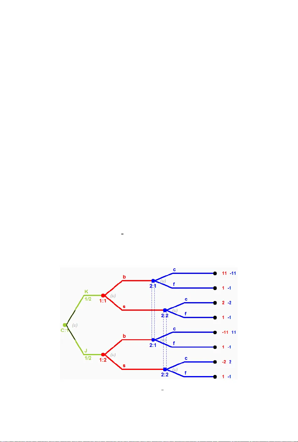
Bayesian Opponent Exploitation in Imperfe ct-Information Games SAM GANZFRIED, Florida International University and Ganzfried Research QINGY UN SUN, Stanford University T wo fundamental problems in computational game theory are computing a Nash equilibrium and learning to exploit opponents given observations of their play (opponent exploitation). e laer is perhaps even more important than the former: Nash e quilibrium does not have a comp elling theoretical justication in game classes other than two-player zer o-sum, and for all games one can potentially do beer by exploiting perceived weaknesses of the opponent than by following a static equilibrium strategy throughout the match. e natural seing for opponent exploitation is the Bayesian seing where we have a prior mo del that is integrated with observations to create a posterior opponent model that we respond to. e most natural, and a well-studied prior distribution is the Dirichlet distribution. An exact polynomial-time algorithm is known for best-responding to the posterior distribution for an opponent assuming a Dirichlet prior with multinomial sampling in normal-form games; how ever , for imperfect-information games the best kno wn algorithm is based on approximating an innite integral without theoretical guarantees. W e present the rst exact algorithm for a natural class of imperfect-information games. W e demonstrate that our algorithm runs quickly in practice and outperforms the best prior approaches. W e also present an algorithm for the uniform prior seing. 1 INTRODUCTION Imagine you are playing a game repeatedly against one or more opponents. What algorithm should you use to maximize your performance? e classic “solution concept” in game theor y is the Nash equilibrium. In a Nash equilibrium σ , each player is simultaneously maximizing his pay o assuming the opp onents all follo w their components of σ . So should we just nd a Nash equilibrium strategy for ourselves and play it in all the game iterations? Unfortunately , there ar e some complications. First, there can exist many Nash equilibria, and if the opponents are not following the same one that we have found (or are not following one at all), then our strategy would hav e no performance guarantees. Second, nding a Nash equilibrium is challenging computationally: it is PP AD-har d and is widely conjectured that no polynomial-time algorithms exist [Chen and Deng, 2006]. ese challenges apply to b oth extensive-form games (of both perfe ct and imperfect information) and strategic-form games, for games with more than two players and non-zero-sum games. While a particular Nash e quilibrium may happen to p erform well in practice, 1 there is no theoretically compelling justication for why computing one and playing it repeatedly is a go od approach. T wo-player zero-sum games do not face these challenges: there exist polynomial-time algorithms for computing an e quilibrium [K oller et al . , 1994], and there exists a game value that is guaranteed in expectation in the worst case by all equilibrium strategies regardless of the strategy played by the opp onent (and this value is the b est worst-case guaranteed payo for any of our strategies). However , e ven for this game class it would b e desirable to deviate from equilibrium in order to learn and exploit perceived weaknesses of the opponent; for instance, if the opponent has played Rock in each of the rst thousand iterations of rock-paper-scissors, it seems desirable to put additional weight on paper beyond the equilibrium value of 1 3 . us, learning to exploit opponents’ weaknesses is desirable in all game classes. One approach would be to construct an opp onent model consisting of a single mixe d strategy that we believe the opponent is playing given our obser vations of his play and a prior distribution (p erhaps computed 1 An agent for 3-player limit T exas hold ’ em computed by the counterfactual r egret minimization algorithm ( which converges to Nash equilibrium in certain games) performed well in practice despite a lack of theoretical justication [Gibson, 2014]. Sam Ganzfried and Qingyun Sun 2 from a database of historical play ). is approach has been successfully applied to exploit weak agents in limit T exas hold ’em poker , a large imperfect-information game [Ganzfried and Sandholm, 2011]. 2 A drawback is that it is potentially not robust. It is very unlikely that the opp onent’s strategy matches this point estimate exactly , and we could p erform poorly if our model is incorrect. A more robust approach, which is the natural one to use in this seing, is to use a Bayesian model, where the prior and posterior are full distributions ov er mixed strategies of the opponent, not single mixed strategies. A natural prior distribution, which has be en studied and applied in this context, is the Dirichlet distribution. e p df of the Dirichlet distribution is the b elief that the probabilities of K rival events are x i given that each event has been obser ved α i − 1 times: f ( x , α ) = 1 B ( α )  x α i − 1 i . 3 Some notable properties are that the mean is E [ X i ] = α i  k α k and that, assuming multinomial sampling, the posterior aer including new obser vations is also Dirichlet, with parameters updated based on the new obser vations. Prior work has presented an ecient algorithm for optimally exploiting an opp onent in normal- form games in the Bayesian seing with a Dirichlet prior [Fudenberg and Levine, 1998]. e algorithm is essentially the ctitious play rule [Brown, 1951]. Given prior counts α i for each opponent action, the algorithm increments the counter for an action by one each time it is observed, and then best responds to a model for the opponent where he plays each strategy in proportion to the counters. is algorithm would also extend dir ectly to sequential extensive-form games of perfect information, where we maintain independent counters at each of the opponent’s decision nodes; this would also work for games of imperfect information where the opponent’s private information is observed aer each round of play (so that we w ould know exactly what information set he took the obser ved action from). For all of these game classes the algorithm would apply to both zero and general-sum games, for any number of players. However , it would not apply to imperfect-information games where the opponent’s private information is not obser ved aer play . An algorithm e xists for approximating a Bayesian best response in imperfect-information games, which uses importance sampling to approximate an innite integral. is algorithm has been successfully applie d to limit T exas hold ’em poker [Southey et al . , 2005]. 4 Howev er , it is only a heuristic approach with no guarantees. e authors state, “Computing the integral over opp onent strategies dep ends on the form of the prior but is dicult in any event. For Dirichlet priors, it is possible to compute the posterior exactly but the calculation is expensive except for small games with relatively few obser vations. is makes the exact BBR an ideal goal rather than a practical approach. For real play , we must consider approximations to BBR. ” Howev er , we see no justication for the claim that it is possible to compute the posterior exactly in prior work, and there could easily be no closed-form solution. In this paper we present a solution for this problem, leading to the rst exact optimal algorithm for performing Bayesian opponent exploitation in imperfect-information games. While the claim is corr ect that the computation is expensive for large games, we show that in a small (yet realistic) game it outperforms all prior approaches. Furthermore, we sho w that the computation can run extremely quickly even for large number of observations (though it can run into numerical instability), contradicting the second claim. W e also present general theory , and an algorithm for another natural prior distribution (uniform distribution over a polyhedron). 2 is approach used an approximate Nash equilibrium strategy as the prior and is applicable ev en when historical data is not available , though if additional data were available a mor e informed prior that capitalizes on the data would b e pr eferable. 3 B ( α ) is the beta function B ( α ) =  Γ ( α i ) Γ (  i α i ) , where Γ ( n ) = ( n − 1 ) ! is the gamma function. 4 In addition to Bayesian Best Response, the paper also considers heuristic approaches for approximating several other response functions: Max A Posteriori Response and ompson’s Response. Sam Ganzfried and Qingyun Sun 3 2 MET A - ALGORITHM e problem of developing ecient algorithms for optimizing against a posterior distribution, which is a probability distribution o ver mixed strategies for the opponent (which are themselv es distributions over pure strategies) seems daunting. W e need to b e able to compactly represent the posterior distribution and eciently compute a b est response to it. Fortunately , we show that our payo of playing any strategy σ i against a probability distribution over mixed strategies for the opponent equals our payo of playing σ i against the mean of the distribution. us, we ne ed only represent and respond to the single strategy that is the mean of the distribution, and not to the full distribution. While this result was likely known previously , we have not se en it stated explicitly , and it is important enough to be highlighted so that it is on the radar of the AI community . Suppose the opponent is playing mixe d strategy σ − i where σ − i ( s − j ) is the probability that he plays pure strategy s − j ∈ S − j . By denition of expected utility , u i ( σ i , σ − i ) =  s − j ∈ S − j σ − i ( s − j ) u i ( σ i , s − j ) . W e can generalize this naturally to the case where the opponent is playing according to a probability distribution with pdf f − i over mixed strategies: u i ( σ i , f − i ) =  σ − i ∈ Σ − i [ f − i ( σ − i ) · u i ( σ i , σ − i ) ] . Let f − i denote the mean of f − i . at is, f − i is the mixed strategy that selects s − j with probability  σ − i ∈ Σ − i  σ − i ( s − j ) · f − i ( σ − i )  . en we have the following: Theorem 2.1. u i ( σ i , f − i ) = u i ( σ i , f − i ) . at is, the payo against the mean of a strategy distribution equals the payo against the full distribution. Proof. u i ( σ i , f − i ) =  s − j ∈ S − j  u i ( σ i , s − j )  σ − i ∈ Σ − i  σ − i ( s − j ) · f − i ( σ − i )   =  s − j ∈ S − j   σ − i ∈ Σ − i  u i ( σ i , s − j ) · σ − i ( s − j ) · f − i ( σ − i )   =  σ − i ∈ Σ − i        j ∈ S − j  u i ( σ i , s − j ) · σ − i ( s − j ) · f − i ( σ − i )        =  σ − i ∈ Σ − i [ u i ( σ i , σ − i ) · f − i ( σ − i ) ] = u i ( σ i , f − i )  eorem 2.1 applies to both normal and extensive-form games (with perfect or imperfect infor- mation), for any number of players ( σ − i could be a joint strategy prole for all opposing agents). Now suppose the opponent is playing according a prior distribution p ( σ − i ) , and let p ( σ − i | x ) denote the posterior probability given observations x . Let p ( σ − i | x ) denote the mean of p ( σ − i | x ) . As an immediate consequence of eorem 2.1, we have the following corollary . Sam Ganzfried and Qingyun Sun 4 Corollary 2.2. u i ( σ i , p ( σ − i | x )) = u i ( σ i , p ( σ − i | x )) . Corollary 2.2 implies the meta-procedure for optimizing p erformance against an opponent who uses p given by Algorithm 1. Algorithm 1 Meta-algorithm for Bayesian opponent exploitation Inputs : Prior distribution p 0 , response functions r t for 0 ≤ t ≤ T M 0 ← p 0 ( σ − i ) R 0 ← r 0 ( M 0 ) Play according to R 0 for t = 1 to T do x t ← obser vations of opponent’s play at time step t p t ← p osterior distribution of opponent’s strategy given prior p t − 1 and observations x t M t ← mean of p t R t ← r t ( M t ) Play according to R t ere are sev eral challenges for applying Algorithm 1. First, it assumes that we can compactly represent the prior and posterior distributions p t , which have innite domain (the set of opponents’ mixed strategy proles). Second, it requires a procedure to eciently compute the posterior distributions given the prior and the observations, which requires updating potentially innitely many strategies. ird, it requires an ecient procedure to compute the mean of p t . And fourth, it requires that the full posterior distribution from one round b e compactly represented to b e used as the prior in the next round. W e can address the fourth challenge by using a modied update step: p t ← posterior distribution of opponent’s strategy given prior p 0 and observations x 1 , . . . , x t . W e will be using this new rule in our main algorithm. e response functions r t could b e standard best response, for which linear-time algorithms exist in games of imperfect information (and a recent approach has enabled ecient computation in extremely large games [Johanson et al . , 2011]). It could also be a more robust response, e.g., one that places a limit on the exploitability of our own strategy , perhaps one that varies over time based on our performance (or a lower-variance estimator of it) [Ganzfried and Sandholm, 2015, Johanson and Bowling, 2009, Johanson et al . , 2007]. In particular , the restricted Nash response has been demonstrate d to outperform best response against agents in limit T exas hold ’ em whose actual strategy may dier substantially from the exact model [Johanson et al., 2007]. 3 ROBUSTNESS OF THE APPROA CH It has been p ointed out that, empirically , the approach described is not robust: if we play a full best response to a point estimate of the opponent’s strategy we can have very high exploitability ourselves, and could perform very p oorly if in fact we are wrong about our mo del [Johanson et al . , 2007]. is could happen for several reasons. Our modeling algorithm could be incorrect: it could make an incorrect assumption about the prior and form of the opp onent’s distribution. is could happen for several reasons. One r eason is that the opp onent could actually b e changing his strategy over time (possibly either by improving his o wn play or by adapting to our play), in which case a model that assumes a static opp onent could be predicting a strategy that the opp onent is no longer using. e opponent could also have modie d his play strategically in an aempt to de ceive us by playing one way initially and then counter-exploiting us as we aempt to exploit the mo del we have formed fr om his initial strategy (e.g., the opp onent initially starts o playing extr emely Sam Ganzfried and Qingyun Sun 5 conservatively , then switches to a more aggressive style as he suspects we will start to exploit his extreme conservatism). His initial strategy ne ed not arise from de ception: it is also p ossible that simply due to chance events ( either due to his own randomization in his strategy or due to the states of private information selected by chance) the opponent has appeared to be playing in a certain way (e.g., very conser vatively), and as he be comes aware of this conser vative “image, ” naturally it occurs to him to modify his play by be coming more aggressive . A second reason that we could be wrong in our opponent model other than our mo deling algorithm incorrectly modeling the opponents’ dynamic approach is that our observations of his play are very noisy (due to both randomization in the opponent’s strategy and to the private information selected by chance), particularly over a small sample. Even if our approach is correct and the opponent is in fact playing a static strategy according to the distribution assumed by the modeling algorithm, it is very unlikely that our actual perception of his strategy is precisely correct. A third reason, of course , is that the opponent may be following a static strategy that does not exactly conform to our model for the prior and/or sampling metho d used to generate the p osterior . W e would like an approach that is robust in the event that our model of the opp onent’s strategy is incorrect, whichever the cause may be. Prior work has considered a model where the opponent plays according to a model x − i with probability p and with probability 1 − p plays a nemesis to our strategy [Johanson et al . , 2007]. For carefully selected values of p (typically 0.95 or 0.99), they show that this can achieve a relatively high level of e xploitation (similar to a full best response) with a signicantly smaller worst-case exploitability . W e note that, as describ ed in Section 2, Algorithm 1 can be integrated with any response function, not ne cessarily a full best response, and so r t could be selected to b e the Restricted Nash Response from prior work [Johanson et al . , 2007]. Howev er , it seems excessively conservative to give the opponent credit for playing a full nemesis to our strategy; if we are relatively condent in our opponent model, then a more reasonable robustness criterion would be to explore performance as we allow the opponent’s strategy to dier by a small amount from the predicted strategy (i.e., the opponent is playing a strategy that is very close to our model, and not necessarily puing weight on a full nemesis to our strategy). Suppose we believe the opponent is playing x − i , while he is actually playing x 0 − i . Let M be the maximum absolute value of a utility to player i , and let N be the maximum numb er of actions available to a player . Let ϵ > 0 b e arbitrary . en, if | x − i ( j ) − x 0 − i ( j ) | < δ for all j , where δ = ϵ M N , | u i ( σ ∗ , x − i ) − u i ( σ ∗ , x 0 − i ) | =       j ( x − i ( j ) − x 0 − i ( j )) u i ( σ ∗ , s − j )      < =  j    x − i ( j ) − x 0 − i ( j )  u i ( σ ∗ , s − j )   < =  j    x − i ( j ) − x 0 − i ( j )   ·   u i ( σ ∗ , s − j )    < =  j  | x − i ( j ) − x 0 − i ( j ) | · M  < M  j δ < = M N δ = M N · ϵ M N = ϵ is same analysis can be applie d directly to show that our payo is continuous in the opp onent’s strategy for many popular distance functions (i.e ., for any distance function where one strategy can get arbitrarily close to another as the components get arbitrarily close). For instance this would apply to L1, L2, and earth mover’s distance, which have be en applied previously to compute distances been strategies within opponent exploitation algorithms [Ganzfried and Sandholm, 2011]. us, if we are slightly o in our model of the opp onent’s strategy , even if we are doing a full best response we will do only slightly worse . Sam Ganzfried and Qingyun Sun 6 4 EXPLOIT A TION ALGORITHM FOR DIRICHLET PRIOR As describe d in Section 1 the Dirichlet distribution is the conjugate prior for the multinomial distribution, and therefore the p osterior is also a Dirichlet distribution, with the parameters α i updated to reect the new observations. us, the mean of the p osterior can be computed eciently by computing the strategy for the opponent in which he plays each strategy in pr oportion to the updated weight, and Algorithm 1 yields an e xact ecient algorithm for computing the Bayesian best response in normal-form games with a Dirichlet prior . However , the algorithm do es not apply to games of imp erfect information since we do not obser ve the private information held by the opponent, and therefore do not know which of his action counters w e should increment. In this section we will pr esent a new algorithm for this seing. W e present it in the context of a representative motivating game where the opponent is dealt a state of private information and then takes publicly-observable action. and present the algorithm for the general seing in Section 4.3. W e are interested in studying the follo wing two-player game seing. Player 1 is given private information state x i (according to a pr obability distribution). en he takes a publicly observable action a i . P layer 2 then takes an action aer observing player 1’s action (but not his private information), and b oth players receive a payo. W e are interested in play er 2’s problem of inferring the (assumed stationary) strategy of player 1 aer repeate d observations of the public action taken (but not the private information). Note that this seing is very general. For example , in poker x i could denote the opponent’s private card(s) and a i the amount bet, and in an ad auction x i could denote his valuation (e.g., high or low ), and a i could denote the amount he bids [T ang et al . , 2016]. 4.1 Motivating game and algorithm For concreteness and motivation, consider the follo wing poker game instantiation of this seing, where we play the role of player 2. Let’s assume that in this tw o-player game, player 1 is dealt a King (K) and Jack ( J) with probability 1 2 , while player 2 is always dealt a een. Player 1 is allowed to make a big bet of $ 10 (b) or a small bet of $ 1 (s), and player 2 is allowed to call or fold. If player 2 folds, then player 1 wins the $ 2 pot (for a prot of $ 1); if player 1 bets and player 2 calls then the player with the higher card wins the $ 2 pot plus the size of the bet. Fig. 1. Chance deals player 1 king or jack with probability 1 2 at the green node. Then player 1 sele cts big or small bet at a red node. Then player 2 cho oses call or fold at a blue node. Sam Ganzfried and Qingyun Sun 7 If we observe player 1’s card aer each hand, then w e can apply the approach described ab ove, where we maintain a counter for player 1 choosing each action with each card that is incremented for the sele cted action. However , if we do not obser ve player 1’s card aer the hand (e.g., if we fold), then we would not know whether to incr ement the counter for the king or the jack. T o simplify analysis, we will assume that we never obser ve the opponent’s private card aer the hand (which is not realistic since we would obser ve his card if he bets and we call); we can assume that we do not observe our payo either until all game iterations are complete, since that could allow us to draw inferences about the opp onent’s card. ere are no known algorithms even for the simplied case of fully unobservable opponent’s private information. W e suspect that an algorithm for the case when the opponent’s private information is sometimes observed can be constructed based on our algorithm, and we plan to study this problem in future work. Let C denote player 1’s card and A denote his action. en P ( C = K ) = P ( C = J ) = 1 2 . Let q b | K ≡ P ( A = b | C = K ) denote the probability that player 1 makes a big bet with king, q s | K ≡ P ( A = s | C = K ) denote the probability that player 1 makes a small b et with king, then q s | K = 1 − q s | K . If we were using a Dirichlet prior with parameters α 1 and α 2 , denoted Dir ( α 1 , α 2 ) , (where α 1 − 1 is the number of times that action b has been obser ved with a king and α 2 − 1 is the number of times s has b een obser ved with a king), then the probability density function is f Dir ( q b | K , q s | K ; α 1 , α 2 ) = ( q α 1 − 1 b | K )( q s | K ) α 2 − 1 B ( α 1 , α 2 ) = ( q α 1 − 1 b | K )( 1 − q b | K ) α 2 − 1 B ( α 1 , α 2 ) In general given obser vations O , Bayes’ rule gives the following, where q is a mixed strategy that is given mass p ( q ) under the prior , and p ( q | O ) is the p osterior: p ( q | O ) = P ( O | q ) p ( q ) P ( O ) =  c ∈ C P ( O , C = c | q ) p ( q ) p ( O ) =  c P ( O | C = c , q ) p ( c ) p ( q ) p ( O ) = ( P ( O | K , q ) p ( K ) + P ( O | J , q ) p ( J )) p ( q ) p ( O ) = ( P ( O | K , q ) + P ( O | J , q )) p ( q ) 2 p ( O ) = q O | K p ( q ) + q O | J p ( q ) 2 p ( O ) Assume action b was observed in a new time step but player 1’s card was not. Let α K b − 1 be the number of times we observed him play b with K according to the prior , etc. P ( q | O ) = q α K b b | K ( 1 − q b | K ) α K s − 1 q α J b − 1 b | J ( 1 − q b | J ) α J s − 1 + q α K b − 1 b | K ( 1 − q b | K ) α K s − 1 q α J b b | J ( 1 − q b | J ) α J s − 1 2 B ( α K b , α K s ) B ( α J b , α J s ) p ( O ) e general expression for the mean of a continuous random variable is E [ X ] =  x x P ( X = x ) d x =  x x  y p ( X , Y ) d y d x =  x  y x p ( X , Y ) d y d x Sam Ganzfried and Qingyun Sun 8 Now we compute the mean of the posterior of the opponent’s probability of playing b with J. P ( A = b | O , C = J ) =  q b | J q b | J P ( q b | J | O ) d q b | J =  q b | J  q b | K q b | J P ( q | O ) d q b | K d q b | J p ( O ) =   ( q α K b b | K ( 1 − q b | K ) α K s − 1 q α J b b | J ( 1 − q b | J ) α J s − 1 + q α K b − 1 b | K ( 1 − q b | K ) α K s − 1 q α J b + 1 b | J ( 1 − q b | J ) α J s − 1 ) d q b | K d q b | J 2 B ( α K b , α K s ) B ( α J b , α J s ) p ( O ) = B ( α K b + 1 , α K s ) B ( α J b + 1 , α J s ) + B ( α K b , α K s ) B ( α J b + 2 , α J s ) 2 B ( α K b , α K s ) B ( α J b , α J s ) p ( O ) = B ( α K b + 1 , α K s ) B ( α J b + 1 , α J s ) + B ( α K b , α K s ) B ( α J b + 2 , α J s ) Z e nal equation can be obtained by obser ving that  q b | J  q b | K q α K b b | K ( 1 − q b | K ) α K s − 1 q α J b b | J ( 1 − q b | J ) α J s − 1 B ( α K b + 1 , α K s ) B ( α J b + 1 , α J s ) d q b | K d q b | J =  q b | J q α J b b | J ( 1 − q b | J ) α J s − 1 B ( α J b + 1 , b J )  q b | K q α K b b | K ( 1 − q b | K ) α K s − 1 B ( α K b + 1 , α K s ) d q b | K d q b | J =  q b | J q α J b b | J ( 1 − q b | J ) α J s − 1 B ( α J b + 1 , α J s ) 1 d q b | J = 1 , since the integrands are themselves Dirichlet and all probability distributions integrate to 1. Simi- larly   ( q α K b − 1 b | K ( 1 − q b | K ) α K s − 1 q α J b + 1 b | J ( 1 − q b | J ) α J s − 1 ) B ( α K b , α K s ) B ( α J b + 2 , α J s ) = 1 . Leing Z denote the denominator , we have P ( b | O , J ) = B ( α K b + 1 , α K s ) B ( α J b + 1 , α J s ) + B ( α K b , α K s ) B ( α J b + 2 , α J s ) Z (1) where the normalization term Z is equal to B ( α K b + 1 , α K s ) B ( α J b + 1 , α J s ) + B ( α K b , α K s ) B ( α J b + 2 , α J s ) + B ( α K b + 1 , α K s ) B ( α J b , α J s + 1 ) + B ( α K b , α K s ) B ( α J b + 1 , α J s + 1 ) P ( s | O , J ) , P ( b | O , K ) , and P ( s | O , K ) can be computed analogously . As stated earlier , B ( α ) =  Γ ( α i ) Γ (  i α i ) where Γ ( n ) = ( n − 1 ) !, which can be computed eciently . Note that the algorithm we have pr esented applies for the case where we play one more game iteration and collect one additional obser vation. However , it is problematic for the general case we are inter ested in where we play many game iterations, since the p osterior distribution is not Dirichlet, and therefore we cannot just apply the same procedure in the ne xt iteration using the computed posterior as the new prior . W e will need to derive a new expression for P ( b | O , J ) for this seing. Suppose that we have observed the opp onent play action b for θ b times and s for θ s times (in addition to the number of ctitious observations reected in the prior α ), though we do not observe his card. Note that there are θ b + 1 possible ways that he could have played b θ b times: 0 times with K and θ b with J, 1 time with K and θ b − 1 with J, etc. us the expression for p ( q | O ) will have θ b + 1 terms in it instead of two (w e can view θ b + 1 as a constant if we assume that the Sam Ganzfried and Qingyun Sun 9 number of game iterations is a constant, but in any case this is linear in the numb er of iterations). W e study generalization to n private information states and m actions in Section 4.3. W e have the new equation P ( q | O ) =  θ b i = 0  θ s j = 0 q α K b − 1 + i b | K ( 1 − q b | K ) α K s − 1 + j q α J b − 1 + ( θ b − i ) b | J ( 1 − q b | J ) α J s − 1 + ( θ s − j ) 2 B ( α K b , α K s ) B ( α J b , α J s ) p ( O ) Using similar reasoning as above, this giv es P ( b | O , J ) =  θ b i = 0  θ s j = 0 B ( α K b + i , α K s + j ) B ( α J b + θ b − i + 1 , α J s + θ s − j ) Z (2) e normalization term is Z =  i  j [ B ( α K b + i , α K s + j ) B ( α J b + θ b − i + 1 , α J s + θ s − j ) + B ( α K b + i , α K s + j ) B ( α J b + θ b − i , α J s + θ s − j + 1 )] us the algorithm for responding to the opp onent is the following. W e start with the prior counters on each private information-action combination, α K b , α K s , etc. W e keep separate counters θ b , θ s for the number of times we have observed each action during play . en we combine these counters according to Equation 2 in or der to compute the strategy for the opponent that is the mean of the posterior given the prior and observations, and we best respond to this strategy , which gives us the same payo as best responding to the full posterior distribution according to e orem 2.1. ere are only O( n 2 ) terms in the expression in Equation 2, so this algorithm is ecient. 4.2 Example Suppose the prior is that the opp onent played b with K 10 times, played s with K 3 times, played b with J 4 times, and played s with J 9 times. us α K b = 10 , α K s = 3 , α J b = 4 , α J s = 9 . Now suppose we observe him play b at the next iteration. Applying our algorithm using Equation 1 gives p ( b | O , J ) = B ( 11 , 3 ) B ( 5 , 9 ) + B ( 10 , 3 )( 6 , 9 ) Z = 0 . 00116550 · 0 . 00015540 + 0 . 00151515 · 0 . 00005550 = 2 . 65209525 e − 7 Z p ( s | O , J ) = B ( 11 , 3 ) B ( 4 , 10 ) + B ( 10 , 3 )( 5 , 10 ) Z = 0 . 00116550 · 0 . 00034965 + 0 . 00151515 · 0 . 00009990 = 5 . 5888056 e − 7 Z − → p ( b | O , J ) = 2 . 65209525 e − 7 2 . 65209525 e − 7 + 5 . 5888056 e − 7 = 0 . 3218210361 . So w e think that with a jack he is playing a strategy that bets big with probability 0.322 and small with probability 0.678. Notice that previously we thought his probability of being big with a jack was 4 13 = 0 . 308, and had we been in the seing where we always observe his card aer gameplay and observed that he had a jack, the posterior probability would be 5 14 = 0 . 357. An alternative “na ¨ ıve ” (and incorrect) approach would be to increment the counter for α J b by α J b α J b + α K b , the ratio of the prior probability that he b ets big given J to the total prior probability that he bets big. is gives a p osterior probability of him being big with J of 4 + 4 13 14 = 0 . 308 , which diers signicantly from the correct value. It turns out that this approach is actually equivalent to Sam Ganzfried and Qingyun Sun 10 just using the prior: x + x x + y x + y + 1 · x + y x + y = x ( x + y ) + x ( x + y + 1 )( x + y ) = x ( x + y + 1 ) ( x + y + 1 )( x + y ) = x x + y 4.3 Algorithm for general seing W e now consider the general seing where the opponent can have n dierent states of private information according to an arbitrar y distribution π and can take m dierent actions. Assume he is given private information x i with probability π i , for i = 1 , . . . , n , and can take action k i , for i = 1 , . . . , m . Assume the prior is Dirichlet with parameters α i j for the number of times action j was played with private information i (so the mean of the prior has the player selecting action k j at state x i with probability α i j  j α i j ). P ( C = x i ) = π i ; P ( A = k j | C = x i ) = q k j | x i ; q k j | x i ∼ f Dir ( q k j | x i ; α i 1 , . . . , a i m ) =  j q α i j − 1 k j | x i B ( α i 1 , . . . , α i m ) As before, using Bay es’ rule we have p ( q | O ) = P ( O | q ) p ( q ) P ( O ) =  i P ( O , C = x i | q ) p ( q ) p ( O ) =  i P ( O | C = x i , q ) π i p ( q ) p ( O ) = p ( q )  i P ( O | x i , q ) π i p ( O ) =  i P ( O | x i ) p ( q ) π i p ( O ) Now assume that action k j ∗ was obser ved in a new time step, while the opponent’s private information was not observed. P ( q | O ) =  n i = 1  π i q k j ∗ | x i  m h = 1  n j = 1 q α j h − 1 k h | x j  p ( O )  n i = 1 B ( α i 1 , . . . , α i m ) W e now compute the expectation for the posterior probability that the opponent plays k j ∗ with private information x i ∗ as done in Section 4.1. P ( A = k j ∗ | O , C = x i ∗ ) =   q k ∗ j | x ∗ i  n i = 1  π i q k j ∗ | x i  m h = 1  n j = 1 q α j h − 1 k h | x j   p ( O )  n i = 1 B ( α i 1 , . . . , α i m ) =  i  π i  j B ( γ 1 j , . . . , γ n j )  Z , where γ i j = α i j + 2 if i = i ∗ and j = j ∗ , γ i j = α i j + 1 if j = j ∗ and i , i ∗ , and γ i j = α i j otherwise. If we denote the numerator by τ i ∗ j ∗ then Z =  i ∗ τ i ∗ j ∗ . Notice that the product is o ver n terms, and therefore the total number of terms will be exponential in n (it is O( m · 2 n )). Sam Ganzfried and Qingyun Sun 11 For the case of multiple obser ved actions, the p osterior is not Dirichlet and cannot be used directly as the prior for the next iteration. Suppose we have observed action k j for θ j times (in addition to the number of ctitious times indicated by the prior counts α i j ). W e compute P ( q | O ) analogously as P ( q | O ) =  n i = 1  π i  { ρ a b }  m h = 1  n j = 1 q α j h − 1 + ρ j h k h | x j  p ( O )  n i = 1 B ( α i 1 , . . . , α i m ) , where the  { ρ a b } is over all values 0 ≤ ρ ab ≤ θ b with  a ρ ab = θ b for each b , for 1 ≤ a ≤ n , 1 ≤ b ≤ m . W e can write this as  { ρ a b } = θ b  ρ 1 b = 0 θ b − ρ 1 b  ρ 2 b = 0 . . . θ b −  n − 2 r = 0 ρ r b  ρ n − 1 , b = 0 θ b −  n − 1 r = 0 ρ r b  ρ n b = θ b −  n − 2 r = 0 ρ r b . Here, the expr ession for the full posterior distribution P ( q | O ) is P ( q | O ) =  i  π i  { ρ a b }  h B ( α 1 h + ρ 1 h , . . . , α n h + ρ n h )  Z (Note that we could marginalize as before to compute the mean of the posterior strategy for arbitrar y indices ˆ i , ˆ j , but we omit these details to avoid making the formula unnecessarily complicated.) For each b , the number of terms equals the numb er of ways of distributing the θ b observations amongst the n possible private information states, which equals C ( θ b + n − 1 , n − 1 ) = ( θ b + n − 1 ) ! ( n − 1 ) ! θ b ! Hence the total number of terms in the summation is upp er bounded by O  ( T + n ) ! n ! T !  , where T is the total number of game iterations which upper bounds the θ b ’s. Since we must do this for each of the m actions, the total number of terms is O   ( T + n ) ! n ! T !  m  . So the number of terms is exponential in the number of private information states and actions, but polynomial in the numb er of iterations. In the following section, we will lo ok at how to compute the product of beta functions for each term by approximating the product with an exponential of the sum of terms, improving the computation complexity for both the single and multiple observation seings. 4.4 Calculation for product of b eta distributions From the pre vious section, we know that the posterior probability that the opponent plays k j ∗ with private information x i ∗ is P ( A = k j ∗ | O , C = x i ∗ ) =  i  π i  j B ( γ 1 j , . . . , γ n j )  Z , One computational boleneck for computing the posterior pr obability is to compute the product of beta distributions. Now we study the product of beta distributions  j B ( γ 1 j , . . . , γ n j ) . W e will derive an analytical formula so that evaluation of this formula is computationally feasible. W e prov e the following theorem: Theorem 4.1. Dene γ j =  n i = 1 γ i j , then dene the empirical probability distribution ˆ P j ( i ) = γ i j  n i = 1 γ i j = γ i j γ j . Dene the Gamma function Γ ( x ) =  ∞ 0 x z − 1 e − x d x , for integer x , Γ ( x ) = ( x − 1 ) ! . Now Sam Ganzfried and Qingyun Sun 12 dene the entropy of ˆ P i as E ( ˆ P j ) = −  n i = 1 ˆ P j ( i ) ln ˆ P j ( i ) . en we have m  j = 1 B ( γ 1 j , . . . , γ n j ) = exp  m  j = 1  − γ j E ( ˆ P j ) − 1 2 ( n − 1 ) ln ( γ j ) + n  i = 1 ln ( P j ( i )) + d   . Here d is a constant such that 1 2 ln ( 2 π ) n − 1 ≤ d ≤ n − 1 2 ln ( 2 π ) , where ln ( 2 π ) ≈ 0 . 92 . Proof. W e know from the denition of beta function that B ( γ 1 j , . . . , γ n j ) =  n i = 1 Γ ( γ i j ) Γ   n i = 1 γ i j  Let’s use a version of Stirling’s formula with bounds valid for all positive integers z , √ 2 π z  z e  z ≤ Γ ( z + 1 ) = z ! ≤ e √ z  z e  z . erefore, Γ ( z + 1 ) = C ( z ) √ z  z e  z and C ( z ) is between √ 2 π = 2 . 5066 and e = 2 . 71828. And since we want to express the pr oduct of Gamma function, we consider ln Γ ( z ) = z ln z − z − 1 2 ln ( z ) + c ( z ) where c ( z ) is b etween 1 2 ln ( 2 π ) ≈ 0 . 92 and 1. Now we can look at the product of beta functions, m  j = 1 B ( γ 1 j , . . . , γ n j ) = m  j = 1   n i = 1 Γ ( γ i j ) Γ   n i = 1 γ i j   = exp  m  j = 1  n  i = 1 ln Γ ( γ i j ) − ln Γ  n  i = 1 γ i j    Now we want to use Stirling’s formula with bounds and the denition of entropy to reduce the terms in the exponential. m  j = 1  n  i = 1 ln Γ ( γ i j ) − ln  Γ  n  i = 1 γ i j    = m  j = 1  n  i = 1  γ i j ln γ i j − γ i j − ln ( γ i j ) 2 + c ( γ i j )  −  n  i = 1 γ i j ln n  i = 1 γ i j − n  i = 1 γ i j − ln   i γ i j  2 + c  n  i = 1 γ i j    = m  j = 1  n  i = 1 γ i j n  i = 1 γ i j  n i = 1 γ i j ln  γ i j  i γ i j  − n − 1 2 ln  n  i = 1 γ i j  + n  i = 1 ln  n  i = 1 γ i j  i γ i j  + n  i = 1 c ( γ i j ) − c n  i = 1 γ i j  = m  j = 1   − γ j E ( ˆ P j )  − 1 2 ( n − 1 ) ln ( γ j ) + n  i = 1 ln ( P j ( i )) + n  i = 1 c ( γ i j ) − c  n  i = 1 γ i j   = m  j = 1   − γ j E ( ˆ P j )  − 1 2 ( n − 1 ) ln ( γ j ) + n  i = 1 ln ( P j ( i )) + d  . Here n 1 2 ln ( 2 π ) − 1 ≤ d ≤ n − 1 2 ln ( 2 π ) . e rst equation is Stirling’s formula with bounds. e second expands and reorganizes the terms. e third equation applies the denition γ j =  n i = 1 γ i j , the denition of empirical probability Sam Ganzfried and Qingyun Sun 13 distribution ˆ P j ( i ) = γ i j  n i = 1 γ i j , and the denition of entropy for an empirical probability distribution E ( ˆ P j ) = − n  i = 1 ˆ P j ( i ) ln ( ˆ P j ( i )) = − n  i = 1 γ i j  n i = 1 γ i j ln  γ i j  n i = 1 γ i j  . e fourth equation uses the bound of c ( γ i j ) between 1 2 ln ( 2 π ) and 1 on each constant, to get 1 2 ln ( 2 π ) n − 1 ≤ d ≤ n − 1 2 ln ( 2 π ) . erefore , we have m  j = 1 B ( γ 1 j , . . . , γ n j ) = exp  m  j = 1  n  i = 1 ln Γ ( γ i j ) − ln Γ ( n  i = 1 γ i j )   = exp  m  j = 1   − γ j E ( ˆ P j )  − 1 2 ( n − 1 ) ln ( γ j ) + n  i = 1 ln ( P j ( i )) + d    W e remark that the approximation is actually prey tight numerically , since in Stirling’s formula, we get a constant c ( z ) between 1 2 ln ( 2 π ) ≈ 0 . 92 and 1. And in numerical computation we can just take 0 . 92. It would be esp ecially accurate when these γ i j are large, since the lower bound 1 2 ln ( 2 π ) ≈ 0 . 92 is accurate in the asymptotic version of Stirling’s formula. Using this formula, we can evaluate P ( A = k j ∗ | O , C = x i ∗ ) eciently . For a single observation, P ( A = k j ∗ | O , C = x i ∗ ) =  i  π i  j B ( γ 1 j , . . . , γ n j )  Z , =  i  π i exp   m j = 1  − γ j E ( ˆ P j ) − 1 2 ( n − 1 ) ln ( γ j ) +  n i = 1 ln ( P j ( i )) + d    Z , where γ i j = α i j + 2 if i = i ∗ and j = j ∗ , γ i j = α i j + 1 if j = j ∗ and i , i ∗ , and γ i j = α i j otherwise. And the constant d is chosen by 1 2 ln ( 2 π ) n − 1 ≤ d ≤ n − 1 2 ln ( 2 π ) . If we denote the numerator by τ i ∗ j ∗ then Z =  i ∗ τ i ∗ j ∗ . e complexity for computing this posterior is n times the complexity of computing the terms inside the exponential. e complexity of that is mn since the computation for entropy is n , and we sum over m in the outside. erefore, the complexity for computing this posterior is n 2 m . Similarly , in the multiple obser vation case, P ( q | O ) =  i  π i  { ρ }  h B ( γ 1 j , . . . , γ n j )  Z =  i  π i  { ρ } exp   m j = 1  − γ j E ( ˆ P j ) − 1 2 ( n − 1 ) ln ( γ j ) +  n i = 1 ln ( P j ( i )) + d    Z , where γ i j = α i j + ρ i j . And  { ρ } is over all values 0 ≤ ρ ab ≤ θ b with  a ρ ab = θ b for each b , for 1 ≤ a ≤ n , 1 ≤ b ≤ m , as  { ρ } = θ b  ρ 1 b = 0 θ b − ρ 1 b  ρ 2 b = 0 . . . θ b −  n − 1 r = 0 ρ r b  ρ n b = 0 . e complexity for computing this posterior is n 2 m · C ( θ b + n − 1 , n − 1 ) , as the product of the complexity in the previous case n 2 m and the number of ways to write θ b as nite sums of Sam Ganzfried and Qingyun Sun 14 observations of at most n buckets, which is C ( θ b + n − 1 , n − 1 ) . If the upper bound on θ b is T , then as we discussed above, the total number of terms in the summation is upper bounded by O  ( T + n ) ! n ! T !  , where T is the total number of game iterations which upper b ounds the θ b ’s. And the complexity of computing this posterior is O  ( T + n ) ! n ! T ! n 2 m  . us, overall this approach for computing products of the beta function leads to an exponential improvement in the running time of the algorithm for one observation, and reduces the dependence on m for the multiple observation seing from exponential to linear , though the complexity still remains exponential in n and T for the laer . 5 ALGORITHM FOR UNIFORM PRIOR DISTRIBU TION Another natural prior that has b een studied previously is the uniform distribution over a polyhe dron. is can model the situation when we think the opponent is playing uniformly at random within some region of a xed strategy , such as a specic Nash equilibrium or a “population mean” strategy based on historical data. Prior work has used this mo del to generate a class of opponents who are signicantly more sophisticated than opp onents who play uniformly at random over the entire space [Ganzfried and Sandholm, 2015]). For example, in rock-paper-scissors, we may think the opponent is playing a strategy uniformly at random out of strategies that play each action with probability within [0.31,0.35], as opposed to completely random over [0,1]. Let v i , j denote the j th vertex for player i , where vertices correspond to mixed strategies. Let p 0 denote the prior distribution ov er vertices, where p 0 i , j is the probability that play er i plays the strategy corr esponding to verte x v i , j . Let V i denote the number of vertices for player i . Algorithm 2 computes the Bayesian b est response in this seing. Correctness follows straightfor wardly by applying Corollary 2.2 with the formula for the mean of the uniform distribution. Algorithm 2 Algorithm for opponent e xploitation with uniform prior distribution o ver polyhedron Inputs : Prior distribution over vertices p 0 , response functions r t for 0 ≤ t ≤ T M 0 ← strategy prole assuming opponent i plays each vertex v i , j with probability p 0 i , j = 1 V i R 0 ← r 0 ( M 0 ) Play according to R 0 for t = 1 to T do for i = 1 to N do a i ← action taken by player i at time step t for j = 1 to V i do p t i , j ← p t − 1 i , j · v i , j ( a i ) Normalize the p t i , j ’s so they sum to 1 M t ← strategy prole assuming opponent i plays each vertex v i , j with probability p t i , j R t ← r t ( M t ) Play according to R t 6 EXPERIMENTS W e ran experiments on the game described in Se ction 4.1. For the beta function computations we used the Colt Java math librar y . 5 For our rst set of experiments we teste d our basic algorithm which assumes that we observe a single opponent action (Equation 1). W e varied the Dirichlet prior 5 hps://dst.lbl.gov/A CSSoware/colt/ Sam Ganzfried and Qingyun Sun 15 parameters to be uniform in { 1,n } to e xplore the runtime as a function of the size of the prior (since computing larger values of the eta function can be challenging). e results (T able 1) show that the computation is ver y fast even for large n , with running time under 8 microseconds for n = 500. Howev er , we also observe frequent numerical instability for large n . e second row shows the percentage of the trials for which the algorithm produced a result of “NaN” (which typically r esults from dividing zero by zero). is jumps from 0% for n = 50 to 8.8% for n = 100 to 86.9% for n = 200. is is due to instability of algorithms for computing the b eta function. W e used to our knowledge the best publicly available beta function solver , but perhaps there could be a dierent solver that leads to beer performance in our seing ( e.g., it trades o runtime for additional precision). In any case, despite the cases of instability , the results indicate that the algorithm runs extremely fast for hundreds of prior obser vations, and since it is exact, it is the b est algorithm for the seings in which it produces a valid output. Note that n = 100 corresponds to 400 prior obser vations on average since there are four parameters, and that the experiments in previous work used a horizon of 200 hands played in a match against an opponent [Southey et al., 2005]. n 10 20 50 100 200 500 Time 0.0005 0.0008 0.0018 0.0025 0.0034 0.0076 NaN 0 0 0 0.0883 0.8694 0.9966 T able 1. Results of mo difying Dirichlet parameters to b e U { 1,n } over one million samples. First row is average runtime in millise conds. Second row is percentage of the trials that output “NaN. ” W e tested our generalized algorithm from Equation 2 for dierent numbers of obser vations, keeping the prior xed. W e use d a Dirichlet prior with all parameters equal to 2 as has b een done in prior work [Southey et al . , 2005]. W e observe (T able 2) that the algorithm runs quickly for large numbers of observations, though again it runs into numerical instability for large values. As one example, the algorithm runs in 19 milliseconds for θ b = 101, θ s = 100. n 10 20 50 100 200 500 1000 Time 0.015 0.03 0.36 2.101 10.306 128.165 728.383 NaN 0 0 0 0 0.290 0.880 0.971 T able 2. Results using Dirichlet prior with all parameters equal to 2 and θ b , θ s in U { 1,n } averaged over 1,000 samples. First row is average runtime in milliseconds, second row is percentage of trials that produced “NaN. ” W e compared our algorithm against the three heuristics describe d in previous w ork [Southey et al . , 2005]. e rst heuristic Bayesian Best Resp onse (BBR) approximates the opp onent’s strategy by sampling strategies according to the prior and computing the mean of the posterior over these samples, then best-responding to this mean strategy . eir Max A Posteriori Response heuristic (MAP) samples strategies from the prior , computes the posterior value for these strategies, and plays a best response to the one with highest posterior value. ompson’s Response samples strategies from the prior , computes the posterior values, then samples one strategy for the opponent fr om these posteriors and plays a best response to it. For all approaches we used a Dirichlet prior with the standard values of 2 for all parameters. For all the sampling approaches we sampled 1,000 strategies from the prior for each opp onent and used these strategies for all hands against that opponent (as was done in prior work [Southey et al . , 2005]). Note that one can draw samples 6 hps://en.wikipedia.org/wiki/Dirichlet distribution#Random number generation Sam Ganzfried and Qingyun Sun 16 x 1 , . . . , x K from a Dirichlet distribution by rst drawing K independent samples y 1 , . . . , y K from Gamma distributions each with density Gamma ( α i , 1 ) = y α i − 1 i e − y i Γ ( α i ) and then seing x i = y i  j y j . 6 W e also compared against the payo of a full best r esponse strategy that knows the actual mixed strategy of the opponent, not just a distribution over his strategies, as well as the Nash e quilibrium strategy . 7 Note that the game has a value to us (player 2) of -0.75, so negative values are not necessarily indicative of “losing. ” T able 3 shows that our exact Bay esian best response algorithm (EBBR) outperforms the heuristic approaches, as expected since it is optimal when the opponent’s strategy is drawn from the prior (though performance is very similar to BBR and not statistically distinguishable until 25 iterations). BBR performed best out of the sampling approaches, which is not surprising because it is trying to approximate the optimal appr oach while the others are optimizing a dierent objective. All of the sampling approaches outperformed just following the Nash e quilibrium, and as expected all exploitation approaches performed worse than playing a best r esponse to the opponent’s actual strategy . Note that, against an opponent drawn from a Dirichlet distribution with all parameters equal to 2 and no further observations of his play , our best response would be to always call, which gives us expecte d payo of zero. us for the initial column the actual value for EBBR when averaged over all opponents would be zero. Against this distribution the Nash e quilibrium has expected payo − 0 . 375. Algorithm Initial 10 25 EBBR − 0 . 00003 ± 0 . 0003 − 0 . 0004 ± 0 . 0009 0 . 0002 ± 0 . 0008 BBR − 0 . 00003 ± 0 . 0003 − 0 . 0004 ± 0 . 0009 − 0 . 0065 ± 0 . 0008 MAP − 0 . 1649 ± 0 . 0002 − 0 . 2025 ± 0 . 0007 − 0 . 2664 ± 0 . 0007 ompson − 0 . 2098 ± 0 . 0002 − 0 . 2224 ± 0 . 0007 − 0 . 2996 ± 0 . 0007 FullBR 0 . 4975 ± 0 . 0002 0 . 4971 ± 0 . 0006 0 . 4978 ± 0 . 0005 Nash − 0 . 3750 ± 0 . 0000 − 0 . 3749 ± 0 . 0001 − 0 . 3751 ± 0 . 0001 T able 3. Comparison with algorithms from prior work, full best response, and Nash equilibrium using Dirichlet prior with parameters equal to 2. Sampling algorithms use 1000 samples. For initial column we sampled 100 million opp onents from the prior , for 10 rounds we sampled one million, and for 25 rounds 500,000. Results are average winrate per hand over all opponents with 95% confidence inter vals. On the positive side the exploitation approaches (particularly EBBR and BBR) are able to signi- cantly outperform the Nash e quilibrium strategy when given access to a reliable prior distribution; howev er , none of them are able to improve o ver time as a result of additional observations (EBBR and BBR perform around the same with more obser vations while ompson and MAP perform noticeably worse). is indicates that, for this seing at least, just obser ving the opp onent’s public action and not private information is not additionally useful in comparison to the p erformance variance and the noise introduced from sampling. In order to successfully learn beyond the prior in imperfect-information seings, algorithms will need access to some of the opponents’ private information. Previous experiments had also shown that when the sampling approaches are played against opponents drawn from the prior , the winning rates converge, typically very quickly (even with access to the opponent’s private information in certain hands that w ent to showdown ): “e 7 Note that the Nash equilibrium for player 2 is to call a big bet with probability 1 4 and a small bet with probability 1 (the equilibrium for player 1 is to always bet big with a king and to bet big with probability 5 6 with a jack). Sam Ganzfried and Qingyun Sun 17 independent Dirichlet prior is very broad, admiing a wide variety of opponents. It is encourag- ing that the Bayesian approach is able to exploit e ven this weak information to achieve a beer result. ” [Southey et al., 2005] W e also tested the eect of using only 10 samples of the opponent’s strategy for the sampling approaches. e approaches would then have a noisier estimate of the opp onent’s strategy and should achieve low er performance against the actual strategy , though run signicantly faster . Alg Initial 10 25 100 EBBR . 0001 ± . 0003 - . 0003 ± . 0003 . 0002 ± . 0002 - . 0014 ± . 0005 BBR - . 0662 ± . 0003 - . 0902 ± . 0003 - . 1634 ± . 0002 - . 3127 ± . 0004 MAP - . 1699 ± . 0002 - . 2060 ± . 0002 - . 2657 ± . 0001 - . 3082 ± . 0004 ompson - . 2118 ± . 0002 - . 2247 ± . 0002 - . 2844 ± . 0001 - . 3725 ± . 0004 FullBR . 4976 ± . 0002 . 4973 ± . 0002 . 4975 ± . 0001 . 4969 ± . 0003 Nash - . 3750 ± . 0000 - . 3750 ± . 0000 - . 3750 ± . 0000 - . 3750 ± . 0001 T able 4. Comparison of our algorithm with algorithms from prior work (BBR, MAP, Thompson), full best response, and Nash equilibrium using Dirichlet prior with parameters equal to 2. The sampling algorithms each use 10 samples from the opponent’s strategy (as oppose d to 1000 samples from our earlier analysis). For the initial column we sampled 100 million opp onents from the prior , for 10 and 25 rounds we sample d ten million, and 300,000 for 100 rounds. ompson and MAP performed very similarly using 10 vs. 1000 samples (these approaches essentially end up selecting a single strategy from the set of samples to be use d as the model, and the results indicate that they are relativ ely insensitive to the number of samples use d), but BBR performs signicantly worse. While the performance between EBBR and BBR was statistically indistinguishable for 1000 samples, EBBR signicantly outperforms BBR with 10 samples, particu- larly for more iterations. As before the sampling approaches seem to actually perform worse over time as the noise propagates, while the p erformance of EBBR remains about the same. e dropo of BBR is particularly signicant. e results indicate that EBBR would be particularly preferable over the sampling approaches if the number of available samples is small (e.g., due to running time considerations) and as the number of game iterations increases (though eventually EBBR can run into numerical stability issues described earlier). 7 CONCLUSION One of the most fundamental problems in game theor y is learning to play optimally against opponents who may make mistakes. W e presented the rst exact algorithm for performing ex- ploitation in imperfect-information games in the Bayesian seing using the most well-studied prior distribution for this problem, the Dirichlet distribution. Previously an exact algorithm had only been presented for normal-form games, and the b est previous algorithm was a heuristic with no guarantees. W e demonstrated experimentally that our algorithm can b e practical and that it outperforms the best prior approaches, though it can run into numerical stability issues for large numbers of observations. W e presented a general meta-algorithm and new theoretical framework for studying opponent exploitation. Future work can extend our analysis to many important seings. For example, we would like to study the seing when the opponent’s private information is only sometimes obser ved (we expect our approach can b e extended easily to this seing) and general sequential games where the agents can take multiple actions ( which we expect to be hard, as indicated by the analysis in the tech report). W e would also like to extend analysis for any numb er of agents. Our algorithm is Sam Ganzfried and Qingyun Sun 18 not specialized for two-player zero-sum games (it applies to general-sum games); if we are able to compute the mean of the posterior strategy against multiple opp onent agents, then best responding to this strategy prole is just a single agent optimization and can be done in time linear in the size of the game r egardless of the number of opponents. While the Dirichlet is the most natural prior for this problem, we would also like to study other important distributions. W e presented an algorithm for the uniform prior distribution ov er a polyhedron, which could model the situation where w e think the opponent is playing a strategy from a uniform distribution in a region around a particular strategy , such as a spe cic equilibrium or a “population mean” based on historical data. Opponent exploitation is a fundamental problem, and our algorithm and extensions could be applicable to many domains that are modeled as an imp erfect-information games. For example, many security game models have imperfect information, e.g., [Kiekintveld et al . , 2010, Letchford and Conitzer, 2010], and opponent exploitation in se curity games has been a very active area of study , e.g., [Nguyen et al . , 2013, Pita et al . , 2010]. It has also be en proposed recently that opponent exploitation can be important in medical treatment [Sandholm, 2015]. REFERENCES George W . Brown. 1951. Iterative Solutions of Games by Fictitious Play . In Activity Analysis of Production and Allo cation , Tjalling C. Koopmans (Ed.). John Wiley & Sons, 374–376. Xi Chen and Xiaotie Deng. 2006. Seling the Complexity of 2-Player Nash Equilibrium. In Proceedings of the A nnual Symposium on Foundations of Computer Science (FOCS) . Drew Fudenberg and David Levine. 1998. e eor y of Learning in Games . MI T Press. Sam Ganzfried and Tuomas Sandholm. 2011. Game theory-based opp onent modeling in large imp erfect-information games. In Proceedings of the International Conference on Autonomous Agents and Multi- Agent Systems (AAMAS) . Sam Ganzfried and Tuomas Sandholm. 2015. Safe Opponent Exploitation. ACM Transactions on Economics and Computation (TEA C) (2015). Special issue on selected papers from EC-12. Richard Gibson. 2014. Regret Minimization in Games and the Development of Champion Multiplayer Computer Poker-P laying Agents . P h.D. Dissertation. University of Alberta. Michael Johanson and Michael Bowling. 2009. Data Biased Robust Counter Strategies. In International Conference on A rticial Intelligence and Statistics (AIST A TS) . Michael Johanson, Kevin W augh, Michael Bowling, and Martin Zinkevich. 2011. Accelerating Best Resp onse Calculation in Large Extensive Games. In Proceedings of the International Joint Conference on A rticial Intelligence (IJCAI) . Michael Johanson, Martin Zinkevich, and Michael Bowling. 2007. Computing Robust Counter-Strategies. In Procee dings of the A nnual Conference on Neural Information Processing Systems (NIPS) . 1128–1135. Christopher Kiekintveld, Milind T ambe, and Janusz Marecki. 2010. Robust Bayesian Methods for Stackelberg Security Games (Extended Abstract). In Autonomous Agents and Multi- Agent Systems . Daphne Koller , Nimrod Megiddo, and Bernhard von Stengel. 1994. Fast algorithms for nding randomized strategies in game trees. In Proceedings of the 26th ACM Symposium on Theor y of Computing (STOC) . 750–760. Joshua Letchford and Vincent Conitzer . 2010. Computing Optimal Strategies to Commit to in Extensive-Form Games. In Proceedings of the ACM Conference on Electronic Commerce (EC) . anh H. Nguyen, Rong Y ang, Amos Azaria, Sarit Kraus, and Milind T ambe. 2013. Analyzing the Eectiveness of A dversary Modeling in Security Games. In Proceedings of the AAAI Conference on Articial Intelligence (AAAI) . James Pita, Manish Jain, Milind T ambe, Fernando Ord ´ o ˜ nez, and Sarit Kraus. 2010. Robust Solutions to Stackelberg Games: Addressing Bounded Rationality and Limited Observations in Human Cognition. A rticial Intelligence Journal 174, 15 (2010), 1142–1171. T uomas Sandholm. 2015. Steering Evolution Strategically: Computational Game eory and Opponent Exploitation for Treatment Planning, Drug Design, and Synthetic Biology . In Proceedings of the AAAI Conference on A rticial Intelligence (AAAI) . Senior Member Blue Skies Track. Finnegan Southey , Michael Bowling, Br yce Larson, Carmelo Piccione, Neil Bur ch, Darse Billings, and Chris Rayner . 2005. Bayes’ Blu: Opponent Modelling in Poker . In Proce edings of the 21st A nnual Conference on Uncertainty in A rticial Intelligence (U AI) . 550–558. Pingzhong T ang, Zihe W ang, and Xiaoquan Zhang. 2016. Optimal commitments in auctions with incomplete information. In Proceedings of the ACM Conference on Economics and Computation (EC) .