Fuzzy Bayesian Learning

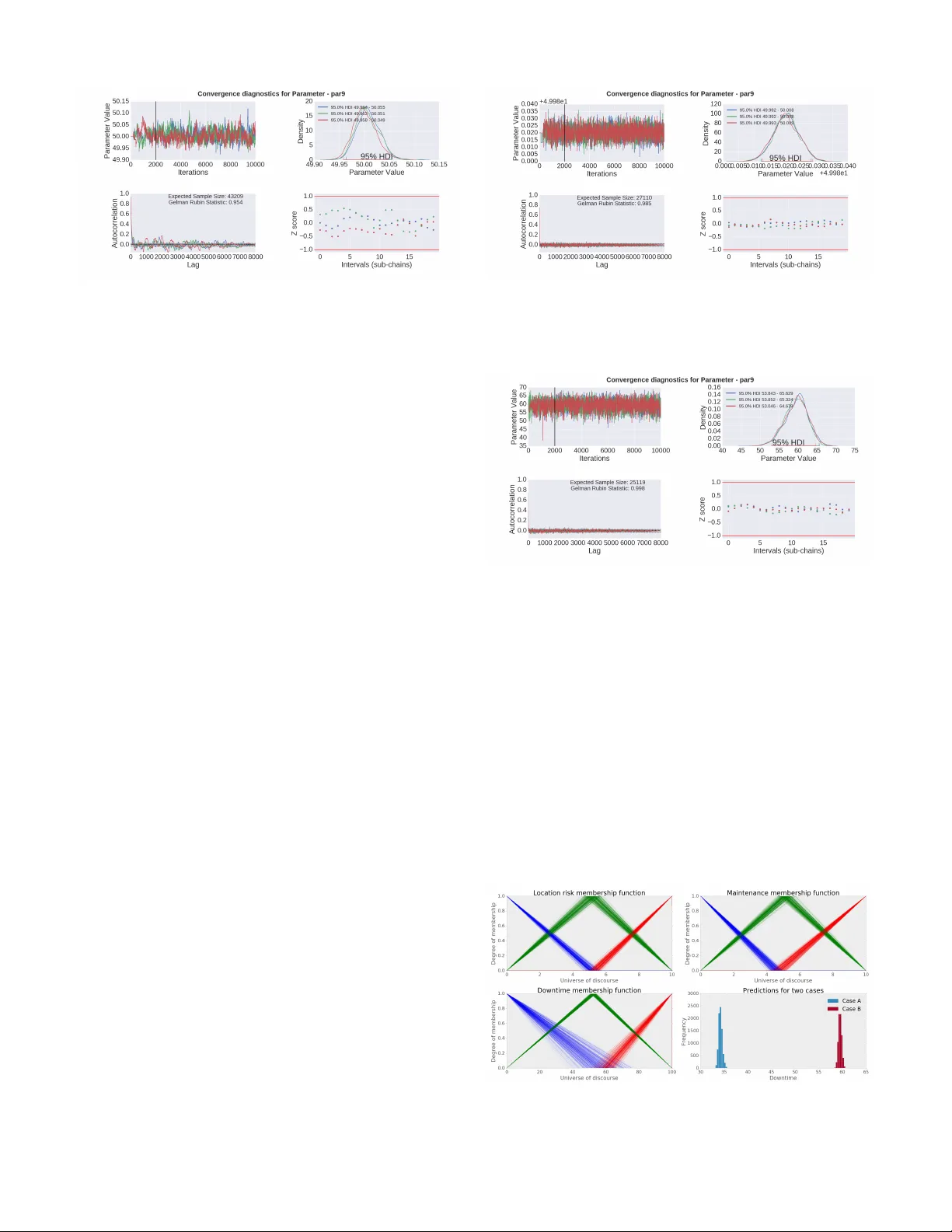
1 Fuzzy Bayesian Learning Indranil Pan and Dirk Bester Abstract —In this paper we propose a novel appr oach for learn- ing from data using rule based fuzzy inference systems where the model parameters are estimated using Bay esian inference and Markov Chain Monte Carlo (MCMC) techniques. W e show the applicability of the method for regression and classification tasks using synthetic data-sets and also a real world example in the financial services industry . Then we demonstrate how the method can be extended for knowledge extraction to select the individual rules in a Bayesian way which best explains the given data. Finally we discuss the advantages and pitfalls of using this method over state-of-the-art techniques and highlight the specific class of problems where this would be useful. Index T erms —fuzzy logic; mamdani method; machine learn- ing; MCMC. I . I N T RO D U C T I O N P R OB ABILITY theory and fuzzy logic hav e been shown to be complementary [1] and various works ha ve looked at the symbiotic integration of these two paradigms [2], [3] including the recently introduced concept of Z-numbers [4]. Historically fuzzy logic has been applied to problems in v olving imprecision in linguistic variables, while probability theory has been used for quantifying uncertainty in a wide range of disciplines. V arious generalisations and extensions of fuzzy sets ha ve been proposed to incorporate uncertainty and vagueness which arise from multiple sources. For example, the type-2 fuzzy [5], [6] sets and type-n fuzzy sets [5] can include uncertainty while defining the membership functions themselves. Intuitionistic fuzzy sets [7] additionally introduce the degree of non-membership of an element to take into account that there might be some hesitation degree and the degree of membership and non-membership of an element might not always add to one. Non-stationary fuzzy sets [8] can model v ariation of opinion ov er time by defining a collection of type 1 fuzzy sets and an explicit relationship between them. Fuzzy multi-sets [9] generalise crisp sets where multiple occurrences of an element are permitted. Hesitant fuzzy sets [10] hav e been proposed from the motiv ation that the problem of assigning a degree of membership to an element is not because of a margin of error (like Atanassov’ s intuitionistic fuzzy sets) or a possibility distribution on possibility values (e.g. type 2 fuzzy sets), but because there is a set of possible values [10]. Formally these can be viewed as fuzzy multi- sets b ut with a different interpretation. Apart from these quantitativ e tools, other approaches have been used to address the vagueness of the qualitativ e meanings used by experts like fuzzy linguistic approaches [11] and various linguistic models hav e been proposed to address this [12]–[14]. I. Pan was with Imperial College London, UK, and now works at Sciemus Ltd, London UK. e-mail: i.pan11@imperial.ac.uk, ipan@sciemus.com D. Bester was with Univ ersity of Oxford, UK, and now works at Sciemus Ltd, London UK. e-mail: dbester@sciemus.com Bayesian inference, on the other hand, provides a method of incorporating the subjectiv e beliefs of the experts about the value of a model parameter , using prior probability dis- tributions, through expert elicitation methods [15]. Howe ver , expert knowledge does not always come in the form of precise probability distributions and often hav e vague and ambiguous statements embodying some form of knowledge [16]. In such cases, both uncertainty and imprecision exist simultaneously [17]. The data is said to be uncertain if the degree of confidence in what is represented by the data is less than one [17], [18]. On the other hand data is imprecise if the implied attrib ute is not singular but belongs to an ill defined set [17], [18]. These two things cannot be discerned if they are represented by a single probability distribution and the contribution of each of these in the final posterior distribution cannot be tracked [19]. Howe v er , fewer works ha ve looked at integration of Bayesian methods with fuzzy logic [20], [21]. For example, [22] attempts to generalise Bayesian methods for samples of fuzzy data and for prior distributions with imprecise param- eters. Recent works have also looked at extension of these works for possibilistic Bayesian inference [23]. Howe v er , in all the above-mentioned literatures, most of the work is on representing the data in terms of fuzzy numbers and optimising model parameters based on that. None of the literatures specifically lev erage on one of the fundamental strengths of the fuzzy inference system, i.e. expressing the expert opinion in terms of rule bases. This is specifically what this paper addresses and the idea stems from the fact that often the experts not only ha ve an opinion on the uncertainty estimates of the model covariates, but also have an intuition of the inter-dependence between the various model cov ariates on the final output. None of the above-mentioned methods take this explicitly into account and hence do not fully exploit the embodied kno wledge provided by the experts. Another line of research has been the use of the belief rule base (BRB) inference methodology as proposed in [24] which uses an expert rule base and assigns a belief degree to each rule, individual rule weights and attribute weights. This treatment is not fully Bayesian and including these additional parameters for characterising these rule bases requires multi- objectiv e optimisation methods to giv e acceptable lev els of performance [25]. Having to estimate more number of param- eters from a small data-set is inherently difficult and would hav e large confidence intervals (using frequentist methods) or large highest density intervals (using Bayesian methods). This issue is addressed in our methodology , since it does not need to have too many additional parameters over and abov e that required by the fuzzy rule base itself. This also helps in reducing the explosion of parameters if higher number of rule bases or fuzzy sets are used. Also the outputs in these 2 works is a belief distribution ov er the fuzzy variables like low , medium and high, instead of a distribution on the crisp output of real numbers, as proposed later in this work. This is important especially if such models are de v eloped as a part of a larger decision making framew ork which relies on probability distributions as outputs from the sub-models. A Bayesian extension of this frame work is proposed in [26] to update the belief degrees based on a recursi v e online estimation. This also addresses a dif ferent problem and has the same issues as the BRB methodology mentioned earlier . Adaptiv e fuzzy systems ha ve been used to approximate non- conjugate priors, likelihoods and approximate hyper-priors in Bayesian inference, which helps in allowing users to extend the inference for a wider range of prior and likelihood prob- ability density functions [27]. In our proposed method, we use Markov Chain Monte Carlo (MCMC) [28] to numerically approximate the posterior distribution and hence do not have the issues relating to conjugacy . Consequently , our method can work on any likelihood or prior distribution. The motiv ation of the present work stems from the need to incorporate linguistic expert opinion within the standard Bayesian framework, so that the end-to-end overall system works on a set of crisp input-output data, which might have probabilistic uncertainties associated with them. It is easier for experts with domain knowledge to come up with a linguistic rule base, but to get good prediction accuracy on any data-set, the shape of the membership functions need to be appropri- ately chosen. The novelty of our work is that we con vert this problem into a Bayesian parameter estimation problem where the shape of the membership functions are estimated through an MCMC algorithm for a given data-set. W e also extend this to Bayesian inference on the individual rules themselves to find out which of the rules are more probable, giv en the data. This approach le verages on the strengths of both the disci- plines – statistics and computational intelligence to come up with a practical solution methodology . In traditional statistics, the emphasis is on parameter estimation for a giv en model structure (which is chosen by the user) from a given set of data-points. In soft computing, the emphasis is on mathemat- ically laying down the imprecision in the spoken language and expert opinions in the form of rule bases and does not need data to generate membership functions at the outset (data might be used later for calibration of the membership functions to impro ve prediction accuracies). Both of these advantages are synergistically used in the present work and the subsequent section de velops this proposition in more detail. I I . P RO P O S E D M E T H O D O L O G Y A N D D E M O N S T R A T I V E E X A M P L E S All empirical modelling approaches which learn from data, like linear and non-linear regression, generalised linear mod- els, neural networks, or kernel based methods like Gaussian processes, support vector machines etc. can be interpreted using a generic Bayesian framew ork as an inference of the underlying non-linear model function g ( x ; θ ) (with parameters θ ), giv en the data. For the set of input vectors X N = x i ∀ i ∈ { 1 , 2 , ..., N } and the set of outputs Y N = y i ∀ i ∈ { 1 , 2 , ..., N } the inference of the function g ( x ; θ ) can be mathematically represented by the posterior probability distribution [29] p ( g ( x ; θ ) | Y N , X N ) = p ( Y N | g ( x ; θ ) , X N ) p ( g ( x ; θ )) p ( Y N | X N ) (1) where, p ( Y N | g ( x ; θ ) , X N ) is the likelihood function which giv es the probability of the output values giv en the function g ( x ; θ ) and the term p ( g ( x ; θ )) is the prior distribution of the functions and its corresponding parameters assumed by the model. As with most other modelling approaches, the abov e equation assumes that the covariates are independent of the model parameters and the functional form of g ( x ; θ ) , i.e., p ( X N | g ( x ; θ )) = p ( X N ) , but the assumption breaks if there is selection bias [15]. Any choice on the parametric structure of the model g ( x ; θ ) , implicitly specifies p ( g ( x ; θ )) in terms of the non-linear relationships among the cov ariates, smoothness, continuity etc. For parametric models like linear regression where the structure of the model g ( x ; θ ) is known, Eq. (1) essentially transforms into an inference only on the model parameters θ giv en by p ( θ | Y N , X N ) = p ( Y N | θ , X N ) p ( θ ) p ( Y N | X N ) (2) For non-parametric approaches, like Gaussian processes, the prior p ( g ( x ; θ )) can be placed directly on the function space without any requirement of explicit parameterisation of the function g ( x ; θ ) . In our case, the function g ( x ; θ ) is a fuzzy inference system gi ven by the rule base Eq. (3) β k R k : if A k 1 ⊕ A k 2 ⊕ . . . ⊕ A k T k then C k (3) where β k is a dichotomous variable indicating the inclusion of the k th rule in the fuzzy inference system, A k i ∀ i ∈ { 1 , 2 , ..., T k } is a referential value of the i th antecedent attribute in the k th rule, T k is the number of antecedent attributes used in the k th rule, C k is the consequent in the k th rule, ⊕ ∈ {∨ , ∧} represents the set of connectiv es (OR, AND operations) in the rules. A referential value is a member of a referential set with the universe of discourse U i , which are meaningful representations for specifying an attrib ute using subjectiv e linguistic terms which are easily understood by an expert. For example, an attribute representing maintenance lev el might consist of linguistic terms like ‘poor’, ‘medium’ and ‘good’. Each of these referential v alues are characterised by membership functions f i ( A i , U i , φ i ) or f i ( C i , U i , φ i ) and for the inference of the function g ( x ; θ ) in Eq. (1), the set of parameters to be estimated is θ , which contains all φ i and β k Remark 1: Since the parameter estimation problem does not impose any specific structure on Eq. (3), the underlying fuzzy rule bases or sets can be defined to be of other types like fuzzy type II, intuitionistic fuzzy sets, hesitant fuzzy sets etc. Remark 2: Including β k in Eq. (3) for selecting each rule and estimating these co-efficients within a Bayesian framew ork, essentially results in knowledge extraction from the data in the form of rules, i.e., the expert has some prior opinion on specific set of rules and the Bayesian inference 3 engine combines the data with this to show which of the ones are more likely given the data. A. Re gr ession on synthetic data-sets 1) Bayesian estimation of fuzzy membership function pa- rameters: Consider the synthetic example of predicting down- time of an engineering process system based on the vari- ables location risk and maintenance lev el. For the refer- ential sets loc r isk, maintenance, dow ntime the referen- tial values are { LO , M E D , H I } , { P OO R, AV G, GO OD } , { LO , M E D , H I } respectively . The corresponding member- ship functions are considered to be triangular and can be mathematically expressed as f i ( u, φ i ) =          ( u − φ i 1 ) ( φ i 2 − φ i 1 ) if φ i 1 ≤ u ≤ φ i 2 ( u − φ i 3 ) ( φ i 2 − φ i 3 ) if φ i 2 ≤ u ≤ φ i 3 0 other wise (4) where, u ∈ U i is any value within the univ erse of discourse and φ i j ∈ φ i ∀ j are the parameters of the membership functions to be estimated by the MCMC algorithm. The rule base used for constructing the fuzzy inference system is as follows: R 1 : if l oc r isk == H I ∨ maintenance == P O OR then dow ntime == H I R 2 : if l oc r isk == M E D ∨ maintenance == AV G then dow ntime == M E D R 3 : if l oc r isk == LO W ∧ maintenance == GOO D then dow ntime == LO W (5) For this case we assume all the rules to be kno wn ( β k = 1 , ∀ k ) and only the parameters ( φ i ) of the membership func- tions ( f i ) need to be estimated. For this example, 100 data points are generated from the rule base in Eq. (5) using triangular membership functions and centroid method of de- fuzzification. The values of the tips and the bases of the trian- gular membership functions are to be estimated by the MCMC algorithm. Therefore, for this case with three referential sets each with three referential attributes, there are 9 parameters to be estimated. Assume the follo wing for the set of observations { Y N , X N } : Y N ∼ MV N  g ( X N ; θ ) , σ 2 I N  , (6) where MV N ( µ , Σ) is the Multiv ariate-Normal distribution with mean vector µ and covariance matrix Σ . The mean vector for our model comes from g ( X N ; θ ) and the fuzzy inference system from Eq. (3). W e use I N , the N × N identity matrix, along with a parameter σ to construct the cov ariance matrix. In other words, the observations of 100 data-points are assumed to come from a normal distribution with the mean ( µ ) of the distribution giv en by the output of the fuzzy inference system and a variance ( σ ) representing the measurement error . This leads to the likelihood p ( y N | g ( x ; θ ) , X N ) = 1 p (2 π ) N σ 2 N × exp  − 1 2 σ 2 N  y N − g ( X N ; θ )  T  y N − g ( X N ; θ )   . (7) where y N is a realisation of the random variable Y N . The set of parameters is θ = { φ i : i = 1 . . . n } where n is the number of parameters to be estimated, and we can estimate it by being Bayesian and assuming a prior p ( θ ) . This giv es the posterior distribution: p ( θ | y N , X N ) ∝ p ( y N | g ( x ; θ ) , X N ) p ( θ ) . (8) Although Eq. (8) is not mathematically tractable, we can draw samples from it using a Metropolis-Hastings algorithm such as the Gibbs sampler [30]. a) Case I: P arameter estimation without measur ement noise and small data set: For this case, since the data-points are generated from the true fuzzy inference system without any addition of noise, we set σ = 0 . 001 , i.e. the measurement error is negligible. W e set the prior p ( θ ) to be independent uniform distributions over the parameter space for each φ i φ i ∼ Uniform (0 , C max ) (9) such that p ( θ ) = p ( φ 1 , φ 2 , . . . , φ n ) = p ( φ 1 ) p ( φ 2 ) . . . p ( φ n ) =  1 C max  n . (10) Here, C max is the maximum allo wed value for the parameter φ i , see table V for the values. The first set of MCMC simulations are run with only 15 data points and the conv ergence diagnostics for one of the parameters (parameter 9) is shown below in Fig. 1. The con ver gence curves for all the others parameters are similar and the Highest Density Intervals (HDIs) are tabulated in T able V in the appendix. For all the simulation cases, non- informativ e priors are used for all the parameters during the Bayesian estimation phase. For all the MCMC simulations in this paper , the python package pymc3 [31] is used. The top left sub-plot in Fig. 1 shows the trace plots for three independent MCMC chains over the parameter space for 10,000 iterations. The burn-in is set at 2000 iterations and is indicated in the figure with a black line. The chains are well mixed and the density plots on the top right are ov erlapping and indicate that they are representativ e of the true posterior distribution. The 95% highest density intervals (HDIs) are also plotted on the x-axis which represent the most probable range of the parameter value. For parameter 9, the true value was 50, and the HDIs for all the three chains are within 49.95 and 50.05, showing that the MCMC algorithm is able to correctly identify the true value of the parameter within a very tight range with only 15 data points. The con v ergence characteristics can also be checked with the 4 Fig. 1. Case I: MCMC conv ergence diagnostics for parameter 9 with 15 data points auto-correlation plots of the three chains on the bottom left. The auto-correlation falls quickly with the number of lags for the post burn-in samples and therefore other methods like chain thinning are not required to obtain a good posterior dis- tribution. The ef fecti ve sample size (ESS) [15] is also reported in this sub-plot which essentially reflects the sample size of a completely non-autocorrelated chain which would yield the same information as the one obtained from the MCMC algorithm. A higher ESS indicates better approximation of the posterior distribution. The Gelman-Rubin statistic or the shrink factor is a measure of the v ariance between the chains relativ e to the variance within the chains. The value for this case, as indicated in the figure, is near 1 which implies that the chains hav e con ver ged. As a thumb rule, if the value is more than 1.1, then there are orphaned or stuck chains. The Z-scores given in the con ver gence diagnostic plots are the Ge weke’ s diagnostic. W e expect these to be from a normal distribution, so most values should be within the red lines in the range [-1,1]. If a substantial amount of the Z-scores fall outside of this, it implies a failure in con ver gence. b) Case II: P arameter estimation without measur ement noise and more data points: The next set of simulations are done with the same settings as the previous case but with 100 data-points instead of 15. The con ver gence characteristics of the same parameter (par9) is sho wn in Fig. 2 and as can be seen in the top right density sub-plot, the 95% HDI is very small around the true value of 50, demonstrating that more data-points help in obtaining much tighter estimates of the parameter values. The trace plots, auto-correlation plots and the Geweke scores indicate that the simulations hav e con ver ged. c) Case III (a): P arameter estimation with additional measur ement noise: For this case, noise from a distribution of N (0 , 1) is added to the 100 observations. The likelihood function for the MCMC in Eq. (6) then has σ = 1 . The con ver gence diagnostics with the density plots for the same parameter (par9) is sho wn in Fig. 3. It can be seen that the HDI of the parameter estimate now spans a much larger region than the two previous simulation runs, due to the noisy data-points. The uncertainty in parameter estimates can be seen from the plots of the membership Fig. 2. Case II: MCMC conv ergence diagnostics for parameter 9 with 100 data points Fig. 3. Case III: MCMC conv ergence diagnostics for parameter 9 with 100 data points and added noise functions obtained by plugging in the v alues from the posterior distribution, as depicted in Fig. 4. It can be observed that for some of the membership function values like the LOW and HI membership function for Downtime, the uncertainties are much higher than the other ones. This might indicate that either there were not enough samples in that region to hav e more tighter estimates for these membership functions, or due to the non-linear nature of the fuzzy rule base, the output variable (Do wntime) and its membership functions have more flexibility and can map the final output for a wider range of parameters. Fig. 4. Posterior of the membership functions and predictive distrib ution for two cases A and B. Fuzzy sets with blue colour indicate LO or POOR, green colour indicate MED or A VG and red colour indicate HI or GOOD. 5 The bottom right sub-plot in Fig. 4 shows the predictions of the Downtime for two different scenarios (Cases A and B). For Case A, the input variables are set to [1.1,8.8] for location risk and maintenance respectively . For Case B, the values are set to [7.7,1.1]. Therefore, in Case A the input suggests that the location risk is low while the maintenance is good. Hence we would intuitiv ely expect the downtime to be low . For case B, the values suggest that the location risk is high and the maintenance is poor . Hence we would intuitiv ely expect the Downtime to be high. This is confirmed by looking at the predictions obtained from the posterior samples as shown in the histograms at the bottom right sub-plot in Fig. 4. For Case A, the Downtime is low with a distribution around 34 and for Case B, the Do wntime is high with a distribution around 59. Once the parameter estimates are obtained, the prediction ov er the whole universe of discourse for all the variables can be obtained along with the posterior distribution of the uncer- tainty at each point as shown in Fig. 11 in the supplementary materials. d) Case III (b): P arameter estimation with additional measur ement noise, when the noise parameter is unknown: This case is similar to Case III (a), except that we assume σ , the noise parameter , is unknown and has to be estimated along with the rest of the parameters. In the estimation, a vague prior ( σ ∼ Uniform (0 . 01 , 10) ) is used. The results sho w that the MCMC algorithm is able to identify the true v alue of σ to reasonably good accuracy with tight HDI bounds. The parameters of the fuzzy membership functions themselves are also identified, though the uncertainty bounds on them (as measured through HDI) are a bit larger than Case III (a), where the value of σ was specified to the true value. This matches with our intuitive understanding of the problem; adding more parameters while keeping the amount of data constant leads to more uncertainty in the estimates. Thus, the FBL technique is not o verly sensitiv e to the value of σ in the present simulation. Care has to be taken with σ ’ s prior . If it is completely erroneous (e.g. range of prior does not include the true value etc.), then the algorithm would fail (or giv e completely erroneous results); as is the case for any Bayesian analysis with wrong priors. In cases where the signal to noise ratio is too lo w , estimating the value of σ would be difficult and the analysis would not provide useful outputs. 2) Bayesian rule base selection and parameter estimation of membership function (Case IV): Consider the case where the dataset is generated as before from the three rules in Eq. (5), but two additional spurious rules are considered while estimating the parameters using MCMC. They are gi ven by: R 4 : if l oc r isk == LO then dow ntime == H I R 5 : if maintenance == P OO R then dow ntime == LO W (11) Clearly these two rules are contrary to our intuition of maintenance and breakdown ev ents mapped on to system downtime and are antagonistic to the original three rules given by Eq. (5). For this case, we set up the MCMC to not only select the parameters of the membership functions ( φ i ) but also the β k in Eq. (3) which indicates the specific rules to be included for best explaining the dataset. Follo wing the lines of [32], we set up a reversible jump MCMC by assuming a prior on the β k parameters, which controls the inclusion of rule k . W e assume that the inclusion of any rule is independent of the inclusion of other rules, and that rules are equally likely to be included as excluded. Probabilistically , this is represented as: β k ∼ Bernoulli (0 . 5) (12) and the β k parameters can be sampled from the posterior distribution along with the other parameters. As before, we ran the MCMC algorithm for 10,000 itera- tions and the con ver gence diagnostics of the same parameter (par9) is sho wn in Fig. 5. The effect of the burn-in is clear from the top left plot and the parameter estimates in the top right have a higher variance (compared to the pre vious cases) around the true v alue of 50. This is due to the fact that the same 100 data points are used to estimate the parameters as before, but in this case the number of parameters are greater – 14 parameters (9 parameters for the fuzzy membership functions and 5 parameters for selecting the individual rules) as opposed to just 9 parameters in the previous cases. The algorithm tries to extract more information from the data (more parameters to estimate) and hence the uncertainties in the parameters are higher . More data would decrease uncertainty around the estimates. Fig. 5. Case IV : MCMC con vergence diagnostics of parameter 9 with for the case of rule base selection Since the rule selection parameter is a Bernoulli distribution (essentially 0 or 1 values instead of continuous real values), it is easier to interpret the results from a histogram plot (Fig. 6) of the MCMC samples for these parameters. Fig. 6 shows that the two spurious rules (Rule 4 & 5) were not chosen by the algorithm (most of the MCMC samples for these have zero values) and the other three rules which generated the data (Rule 1, 2, 3) were correctly identified by the algorithm (most values are one). A small number of MCMC samples for Rules 4, 5 hav e values of one as well, which is during the initial exploration phase of the MCMC (the plot shows values for all the samples and not just post burn-in) and they quickly con v erge to the true values. 3) FBL for the case of sparse rule bases: Next we show how the FBL can work for inference systems with sparse membership sets and with missing rules like the 6 Fig. 6. Histogram of the rule base selection parameters. All values are binary (0 or 1), and due to the stacked nature of the plot the y appear on the continuum of the abscissa. canonical example of the tomato classification problem as discussed in [33], [34]. The problem with such cases is that the rule bases are incomplete and there are empty spaces between membership functions of the antecedants so that when the membership function of the observation falls in the empty space, no rule is fired and therefore no output or consequent is obtained [34], [35]. Follo wing the example of [33], [34] we define the referential sets colour, r ipeness the referential values { GRE E N , Y E LLOW, RE D } , { U N RI P E , H ALF − RI P E , RI P E } , respectiv ely , using triangular membership functions as in Eq. (4), without any ov erlap. The full rule base is giv en as Eq. (13), which includes all the three rules { R a , R b , R c } from which 100 data points are generated (which serves as the observations) and the MCMC algorithm is run on this rule base and data-set. R a : if col our == GRE E N then r ipeness == U N R I P E R b : if col our == Y E LLO W then r ipeness == H ALF − RI P E R c : if col our == RE D then r ipeness == RI P E (13) The results (posterior of the membership functions) are shown in the top row of Fig. (7) which depicts that the true underlying membership functions can be approximated with the full rule base. The second set of simulations is run with only two rules { R a , R c } and the referential values of Y E LLO W , H ALF − RI P E are deleted from the referential sets col our , r ipeness . The results from the MCMC simula- tions using the previous 100 data points are shown in the bottom ro w of Fig. (7). As can be observed, the empty space for the value Y E LLO W is made up for in the antecedant by significant overlap of the other two sets. Also the empty space for H ALF − RI P E is taken care of by the other two sets in the consequent which are much wider now to cover the whole space. Therefore we can see that in the case of sparse rules and membership functions, the MCMC algorithm automatically adjusts the membership functions in such a way that they cover the empty spaces and does a sort of smart interpolation to best explain the data with the sparse rule-base. Fig. 7. Posterior of the membership functions for the sparse rule base case. Colour coding for membership functions: green, golden and orange colours indicate the referential v alues GREEN, YELLO W and RED respecti vely; blue, gray and maroon indicate UNRIPE, HALF-RIPE and RIPE respectiv ely . Of course, more complicated interpolation rules can be incorporated in FBL if it is desired to have, for example, a triangular-type interpolated conclusion for triangular-type observations as proposed in [34]. The framework proposed here-in is generic to accommodate for such intricacies albeit at the cost of higher model complexity . 4) Algorithmic details of MCMC for FBL and its estimation pr operties: W e present a brief discussion on the computational details of the MCMC algorithm, giv en in algorithm 1. Here, Algorithm 1 MCMC Gibbs Sampling Input: G (Number of samples required), Output: G , Posterior samples of θ 1: θ ← arbitrary starting values  Initialisation 2: for G iterations do 3: for i = 1 to n do  n is number of parameters in θ 4: θ i ← DrawSample( p  θ i | θ /θ i  , θ i ) 5: Store( θ i )  Write to MCMC chain 6: end f or 7: end f or DrawSample() is a function that takes a distribution and an optional current value of θ i , and gives a new sample of θ i from the giv en distribution. The distribution p  θ i | θ /θ i  is the conditional distribution of θ i giv en all other parameters in θ , excluding θ i , where n is the number of parameters in the model: p  θ i | θ /θ i  = p  θ i   θ 1 , . . . , θ i − 1 , θ i +1 , . . . , θ n  . This will be proportional to the joint distribution: p  θ i | θ /θ i  = p ( θ 1 , . . . , θ n ) p ( θ 1 , . . . , θ i − 1 , θ i +1 , . . . , θ n ) ∝ p ( θ 1 , . . . , θ n ) . The proportionality is important, since the DrawSample() function is usually the Metropolis-Hastings algorithm (or one of its deriv ates), which only requires the target density to a normalising constant. In our case, this means we hav e to 7 pass the density in Eq. (8) to DrawSample(), which includes g ( x ; θ ) . The DrawSample() function usually in v olves propos- ing new values, and accepting/rejecting these values, as shown in algorithm 2. Candidates for the DrawSample() function Algorithm 2 Sample from arbitrary density function 1: procedur e D R AW S A M P L E ( p ( · ) , θ current ) 2: for L iterations do  Some limit to avoid infinite loop 3: Propose ne w sample θ new using θ current 4: Calculate acceptance probability using p ( θ new ) and p ( θ current ) 5: if Ne w sample accepted then 6: retur n θ new 7: end if 8: end f or 9: retur n θ current 10: end procedur e include Metropolis-Hastings and Slice sampling. When com- paring the GLM to the fuzzy model, the only difference is the specification of g ( x ; θ ) . The GLM has a simple function, defined in terms of a link function and a linear equation and is computationally inexpensiv e since the predictions can be made using efficient matrix multiplications. The fuzzy model has to re-compile each time the rule-base or its parameters changes, which is more computationally expensiv e. T o demonstrate the scaling of the MCMC algorithm with FBL in terms of computational time, we construct two differ- ent cases - (i) v arying the number of estimation parameters and (ii) v arying number of rules in the rule base. F or case (i), the 15 data points are generated using the rules in Eq. (5) as in Case I of section (II-A1a). Dummy estimation variables are added in the MCMC code so that the problem dimension increases but only nine of the original v ariables actually contribute to the fuzzy function. For case (ii), dummy input v ariables are added to the fuzzy inference system with fixed membership functions with dummy rules, so that the complexity of the rule base increases, but number of estimation parameters remain the same. MCMC simulations are performed for 5000 iterations for each case on a 2.40 GHz Intel Xeon CPU with 16 cores and 24 GB RAM running Ubuntu 14.04 Server . The mean of three independent runs are reported in Fig. (8) which sho ws that the computational time increases in a near exponential fashion with the number of rules in the fuzzy inference system while the increase is almost linear with respect to the number of parameters to be estimated by MCMC. This implies that there is more room for improvement of o verall computational time by speeding up the fuzzy function ev aluation. In our synthetic example (Case I in Sec. II-A1a), we knew the true parameter values, thus we used a simulation study with 30 generated datasets to check if we were consistently ov er or underestimating the true parameters, using the pos- terior probability p ( θ < θ true |{ Y N , X N } ) calculated from the MCMC chains for each parameter . W ith no systematic bias, these probabilities should adhere to a Uniform (0 , 1) distribution. W e used a Chi-squared test on our posterior probability estimates, and it did not reject the null hypothesis Fig. 8. Comparison of computation times with respect to number of estimation parameters and rule base complexity of a uniform distribution, showing that the estimates do not hav e a systematic bias. 5) Comparison of the method with Generalised Linear Models (GLM) using Bayesian parameter estimation: T o show the ef fecti veness of the proposed method, we compare four GLM structures with Bayesian parameter estimation. A GLM is composed of the following three elements: an error distribution, a link function, and a linear predictor [36]. W e use the normal distrib ution as our error distribution: Y i ∼ N  µ, σ 2  (14) W e use the identity link function to link the expected value to the linear predictor . W e test four GLMs, with linear predictors as giv en by the following equations, where α i ∀ i are the parameters to be estimated using MCMC. GLM 1 : µ = α 0 + α 1 x 1 + α 2 x 2 (15) GLM 2 : µ = α 0 + α 1 x 1 x 2 (16) GLM 3 : µ = α 0 + α 1 x 2 1 + α 2 x 2 2 + α 3 x 1 x 2 (17) GLM 4 : µ = α 0 + α 1 x 1 + α 2 x 2 + α 3 x 2 1 + α 4 x 2 2 + α 5 x 1 x 2 (18) For the MCMC sampling, the priors on the parameters were σ ∼ half-Cauchy (10) and α i ∼ N (0 , 20) ∀ i , which are noninformativ e priors, ensuring that most of the information would come from the data. The half-Cauchy distribution is defined as the Cauchy distribution left-truncated at zero, as giv en in [37]. The number of MCMC iterations are set to 2,000 and the burn-in as 500. The results are checked for con ver gence as before and the posterior samples after b urn-in are plugged in to each of the GLMs and a distribution of the Downtime predictions ov er the whole 2D surface of Location Risk and Maintenance is obtained. The mean of these surfaces is plotted superimposed with the interpolated surface of the data points as sho wn in Fig. 9. As can be observed from Fig. 9, as more interactions and parameters are added in the GLM structure, it has more flexibility in fitting the data and consequently the fits are better , with GLM4 gi ving the closest fit among all others. Ho we ver , as can be seen from the actual structure of GLM4 in Eq. 18, not much can be gleaned to relate to the expert opinions as 8 Fig. 9. Comparison of the mean surface of the predictions (red surface) from GLM posteriors with the interpolated surface of the actual data-points expressed in Eq. 5 from which the data was generated. In essence, the GLM is one of the many proxies that can fit the data. Also since the surface plots are interpolated from the data-points themselves, they are an approximation of the real surface which generated the data and would be more closer to the real one as and when more data-points are gathered. This might also imply that as more data points are gathered, a different GLM structure might fit better . This can also happen with the fuzzy rules where the algorithm has to choose the rules (as sho wn in the previous section), but if the algorithm selects a different fuzzy rule on having more data points, there is a more transparent e xplanation of the dynamics in the model. In short, it is difficult to come up with a GLM model structure to explain such non-linear relationship in the data. In general, modellers experiment with a combination of linear models, models with interactions, models with higher order terms etc. The only way to include expert opinion in a traditional GLM is to use priors on the parameters (which is a lot less flexible that the IF-ELSE structured fuzzy rule base method proposed in the paper). But since the structure of a GLM is decided ad-hoc it is unclear how to transform expert opinions into priors or model parameters. 6) Comparison with other popular fr equentist machine learning methods: For the sake of comprehensi veness, we also compare the FBL method with some of the popular methods in machine learning which are used in a similar way to learn from data and the corresponding results are reported in T able I. W e use the small dataset (15 data points) for training as in Case I of II-A1a and use a test dataset of 5 data points. The Adaptiv e Neuro Fuzzy Inference System (ANFIS) is trained with 3 membership functions for each of the inputs with 30 epochs. The neural network is trained with a Lev enberg-Marquardt algorithm, has a single hidden layer with 10 neurons and 2 neurons in cases A and B respectiv ely . The support vector regressor (SVR) is trained with a radial basis function kernel. The key issue is that all of the other methods give point estimates and not probabilistic predictiv e distributions (like the FBL). Therefore the mean of the predictiv e distribution from the FBL is used to calculate the MSE (mean squared error) of prediction to compare the performance with other methods. There is no way to compare the uncertainties of the predictions. The results in T able I show that in most of the methods the training MSEs are generally quite low (due to the small dataset), but the test MSEs are much higher (i.e. methods do not generalise well to unseen data). The neural net A case is much worse than neural net B in test MSE due to higher number of neurons (it actually has more parameters than data points which would result in ov erfitting). None of the neural net or SVR giv es rule bases like FBL or ANFIS. The ANFIS rule bases have the additional problem that they are generated from the data and are not always intuiti ve. The FBL method giv es good train and test MSE since the rule base is correctly specified, which might not always be the case in real world cases as discussed later in Section III-E. T ABLE I C O MPA R IS O N O F M E AN S QU A RE D P RE D I C TI O N E R RO R S F O R T H E F U Z Z Y B AY ES I A N M O D EL W I TH OT H E R M AC H I NE L E A RN I N G M E T HO D S Model Prediction T ype T rain MSE T est MSE ANFIS Point predictions 3 . 84 × 10 − 9 7.857 SVR Point predictions 2 . 31 × 10 − 2 1 . 22 Neural Net A Point predictions 7 . 31 × 10 − 2 10.378 Neural Net B Point predictions 5 . 38 × 10 − 1 0.810 FBL Predictiv e distribution 5 . 93 × 10 − 5 7 . 64 × 10 − 5 B. Classification on synthetic data-sets Our modelling methodology for regression can be easily extended for classification tasks. This extension is quite similar to using a logistic regression as a binary classifier . The binary classification task can be defined in terms of a Bernoulli likelihood function whose parameter ( ψ ) is set by the fuzzy inference system ( g ( · ) ) as shown in Eq. 19. Y N ∼ Bernoulli ( ψ ) ψ = g ( X N ; θ ) (19) The rationale for this model for the classification task, is that the Bernoulli distribution gi ves either a one or a zero value (essentially representing the output class) depending on the probability parameter ψ . The fuzzy function acts like a non- linear link function by taking in the input vectors X N and transforming it into a value in the range [0,1] using the pre- specified rule base and the corresponding parameters θ . The rule bases are specified as before (or can be learned using the rule base selection parameter) and the parameters of the fuzzy function can be estimated using the MCMC algorithm. As an illustrative example, we use the same rule base as in Eq. 5 where the input co-variates are in the range [0-10], but the output is in the range [0,1] using triangular membership functions as in Eq. 4. W e generate 100 data points from this fuzzy function and set any data point above a threshold of 0.5 to a value of 1 and any data point belo w it to a value of 0. This forms the training data-set for running the MCMC algorithm to see if the true parameters θ of the fuzzy membership function 9 can be recovered which would classify the data-points into the two classes. Fig. 12, in the supplementary materials, sho ws the underlying surface generated with the true parameters θ , with superimposed 100 randomly drawn samples which is used as the training data-set. For the simulations, 10,000 iterations are done for 3 in- dependent chains and vague priors are chosen for θ as also done in all the regression cases. After rejecting 2000 samples for burn-in, the mean of the posterior parameter samples are plugged into the fuzzy function, with 0.5 as the threshold and the predicted class labels is plotted in Fig. 10. Fig. 10. Binary classification results using the mean of the posterior samples in the Fuzzy Bayesian Learning approach. Predictions for Class 1 is in red, class 0 is in blue and the mis-classifications are sho wn with lime circles. One advantage of this method is that the introduction of the fuzzy system acts as a non-linear kernel and helps in classifying data which are not necessarily linearly separable in the feature space. Also, class one (in red) has much more number of data points than the other (blue) and therefore this is the so-called imbalanced data-set case [38]. The method is able to determine the classes without any special modification for imbalanced data-sets (e.g. changing objective function v alues to penalise mis-classification of one class more than the other etc). Howe ver , as explained earlier in the regression cases as well, the ca veat with this method is that the rule bases might not always be trivial to find and choosing a totally wrong rule base would drastically affect the performance of the classifier . Also, the class label prediction plots in Fig. 10 shows that there is a higher mis-classification at the class boundaries where the underlying fuzzy surface transits from greater than 0.5 to less than 0.5. This implies that the underlying fuzzy surface is not estimated properly with 100 data points, unlike the regression cases (with same or less number of data points) where the parameter estimates had really tight bounds. One possible reason might be that since the observations are just integer values (zeros or ones) instead of real numbers, there is less information for the MCMC algorithm to find the actual parameters with tighter uncertainty bounds. C. Application to a r eal world pr oblem 1) Context and backgr ound of the pr oblem: The back- ground of the problem is rooted in the financial services sector , specifically for making risk quantification models for the non- life speciality insurance domains. For this particular example, consider the case of insuring a power plant operation in the ev ent of business interruption (BI) and property damage (PD) due to various risks like fire hazard, machinery breakdown etc. The focus of this paper is specifically the BI which depends on various factors like the reliability of each of the machinery components, redundancy schemes employed, maintenance schedules etc. Therefore, giv en a set of historic data on these co-variates and the corresponding system uptime in a year, it would be possible to fit a simple GLM or other regression models for prediction. The distribution of the system uptime can then be subsequently used in an insurance pricing model to obtain the required premium. This example focuses on better estimation of the system uptime for the insured engineering process. It is possible to build more in volv ed models of such engi- neering process systems in cases where individual failure and repair data of each of the underlying component is av ailable as has been pursued in [39]. Howe ver , many plant operators are reluctant to share data and therefore such data might not be av ailable for all different kind of process plants, to actually make a sizeable population so as to draw a statistical estimate of the failures and reliability of each component. The proposed Fuzzy Bayesian Learning (FBL) method is useful in such scenarios as it starts with some prior knowledge which informs the model parameters and some prior expert opinion which informs the model structure. As data comes in, the parameters can be re-estimated with these observations to get more tighter estimates around the model parameters and consequently predictions with less uncertainties. This case also serves as a validation of the ability to use this kind of modelling for other type of emerging risk areas where no prior insurance product has been offered and consequently there is little or no loss history data that can be used to build a data-driv en model. In such cases, the fuzzy rule base relying on the underwriter’ s opinion without any data can be constructed to giv e a sense of the outputs. Later the Bayesian parameter estimation can be introduced as the actual claims data start coming in. 2) Dataset description: The data-set is collected in-house at Sciemus Ltd. London, for underwriting insurance risks for its power sector business. The data-set consists of 3 variables, which serve as an input to our model – operation & maintenance (O&M), loss history , design & technology & fire risk (DnTnF). These are qualitativ e opinions indicated by the underwriter from the submission document of the specific risk which comes in to get a quotation for insurance. All these variables are on a scale of 0-10 with 0 representing very poor and 10 indicating very good. Since the dataset consists of historical information from the actual underwriting process, it is possible to see which risk actually led to a loss ev ent and a consequent claim, what was the claim amount and the amount of system uptime during the gi ven insurance period. 10 For this problem setting, the actual outcome is the the system uptime (percentage of time the system was working during the insurance period which is typically one year). This is a small data-set and T able IV giv es the summary statistics of the 24 data-points av ailable in it. 3) Simulations: The fuzzy rule base used for simulation is sho wn in T able II. This is extracted from the intuition of the underwriter who believ es that O&M rating is the key to system uptime. This can be seen reflected in the table – e.g. the first rule states that if the O&M is good, then irrespectiv e of the loss history and design factors the system uptime would be high. The rationale behind such a rule is that if the plant engineers know how the plant operates and are very rigorous with the maintenance schedule and monitoring aspects then they might get a few failures no w and then (and hav e some history of losses), but this is inherently a good risk to underwrite. In some cases though, the loss history can be the ov erriding factor , e.g. rule 4 states that if the loss history is good, then the underwriter gives precedence to this over the bad O&M. Similar lines of reasoning are extracted for the other rules as well. It is important to stress that multiple rules are triggered, each to a different extent, inside the fuzzy inference system, for one given antecedent input set. The final output is a combination of all these triggered values. T ABLE II R U L E B AS E F OR T H E F U Z ZY B AY ES I A N M O D EL FI T T ED O N T H E R E A L W OR L D C A S E Antecedents Consequent O&M Loss history DnTnF System uptime Good - - High Good - A verage Medium A verage - - High Bad Good - High Bad Bad Bad Low Nev ertheless, this rule base extraction is not exhaustiv e and neither all the possible model spaces are explored to see if they giv e similar results. A more rigorous approach to this would be Bayesian model comparison which in v olves comparing the evidence of different models to come up with the model that best explains the data. This is an in vestigation in its own right and a digression from the main theme of the paper which aims to introduce Fuzzy Bayesian Learning and therefore is not pursued in this paper . Ho wev er , to sho w the effecti veness of this simple rule base, it is compared with the predictive accuracies of three GLMs (as shown in Eq. 24-26) fitted with MCMC techniques. The generic likelihood as specified in Eq. 14 is used for all the GLMs. The priors on each of the parameters are sufficiently non-informative to let the model learn from the dataset itself. The σ in Eq. 14 is set to a fixed value of 0.25 (as also done while estimating the parameters of the Fuzzy Bayesian model). Ideally this should hav e been estimated from the data-set itself, but estimating the variance with tight uncertainty bounds actually requires large number of data points and hence this is pre-specified to a small value. Doing so implies that we are relying on the linear predictor to explain most of the relationships in the underlying data-set. For comparing among these models the mean squared error (MSE) is used to gauge the predictiv e accuracies. In Bayesian models, prediction of a new set of values ˜ y N is done using the posterior predicti ve distribution: p ( ˜ y N | y N , X N ) = Z p ( ˜ y N , θ | y N , X N ) dθ = Z p ( ˜ y N | θ , y N , X N ) p ( θ | y N , X N ) dθ = Z p ( ˜ y N | θ , X N ) p ( θ | y N , X N ) dθ . (20) Here, p ( ˜ y N | θ , X N ) is the likelihood assumed on the model in Eq. (8), and p ( θ | y N , X N ) is the posterior distribution. Draw- ing samples from the posterior predictive distrib ution is simple when we already have draws from the posterior distribution as provided by the MCMC sampler [15]. W e used the mean of the posterior predictiv e distribution, y pred N = E [ ˜ y N ] as our final prediction and compare it with the real data-point by calculating the mean squared error (MSE): MSE = 1 N  y pred N − y N  T  y pred N − y N  (21) Howe v er , the MSE metric being a single number does not con ve y the uncertainties in the predictions properly , which can be gleaned from the whole posterior distribution of the prediction (but this again is difficult to compare with each other). The data-set is intentionally not divided into a training and a test set to perform hold out cross validation or k-fold cross validation, since this is a small data-set and ideally we would like the model not to lose out on much information so as to estimate the parameters with more certainty . The resulting comparativ e analysis (using MSE as a metric), between the different models on the real world problem is shown in T able III. As can be observed, the Fuzzy-Bayesian model has a better MSE than GLM 5 which has a simple struc- ture, but is worse of f as compared to the other two GLMs (6 and 7). Ho wev er , as discussed before, there is a narrati ve and more open interpretation for why the Fuzzy-Bayesian model works as opposed to the GLMs. Also predicti ve accuracy from such a small data-set is not really indicativ e of the performance of the model on the true underlying process and obtaining a lower MSE on this data-set might not always be the best option in the long run. As already discussed before, with new data points, different GLMs might gi ve lo wer MSEs. Howe v er , if the underlying process can be quantified with the fuzzy rule bases, then this would lead to a good fit in subsequent scenarios. T ABLE III C O MPA R IS O N O F M E AN S QU A RE D P RE D I C TI O N E R RO R S F O R T H E F U Z Z Y B AY ES I A N M O D EL V I S - A - V IS OT H E R G L M S Model MSE GLM 5 0.4098 GLM 6 0.3649 GLM 7 0.3596 Fuzzy Bayesian 0.3654 11 The advantage of FBL in the real world example is that the underwriting insights can make the model better . But the other downside is that if the rules are extracted only from one underwriter , then their o wn biases and risk perceptions might adversely af fect the model. T o alleviate such concerns, the rule base can be constructed by consulting multiple underwriters and as more data comes in, the individual rule selection methodology (as shown in Section II-A2) can be applied in the parameter estimation process to reject the rules that do not describe the data properly . This allows the model to le verage on the expertise of the best underwriters. I I I . D I S C U S S I O N S A N D C H A L L E N G E S A. Relationship with other machine learning methods Most machine learning methods cannot intuiti vely explain the fitted model in terms of the underlying assumptions. For example, a neural network might giv e very good prediction accuracy on a data-set, but not much reasoning can be gleaned from the model, just by looking at the learned weights of the individual neurons. This might work in applications in an auto- mated framework (like recommender systems, user behaviour prediction etc.) where large number of decisions need to be made in very short time scales without human interventions, and the financial liabilities associated with a mis-classification is not that high. Howe ver , in other industries like personalised healthcare/medicine or specifically our real world example of speciality non-life insurance, prediction from a computer model is almost always validated by a human before taking a final decision, since the consequences of such decisions hav e huge financial/le gal implications. In such circumstances, having a deeper insight into why the algorithm actually works (as opposed to a black-box which just spits out gospel) makes it easier to take a decision and is always preferable. This issue is addressed by our proposed framework since the fuzzy rule base deriv ed from the experts is used to inform the model structure for the regression or classification task. Also the associated uncertainties in the predictions would help the human decision maker to either ask for more information (i.e. recommend to do more medical tests for the healthcare case) or arri ve at a different decision altogether due to the higher associated uncertainties (e.g. decide not to insure a specific risk or charge higher premiums to reflect the higher undertaking of risk). The other issue with traditional machine learning methods, is that they require quite significant amount of data to train and cross-validate a model properly . For the real world cases described abo ve, e v en though the expert kno ws the dependence between the co-variates, it is almost always difficult and expensi ve to collect a comprehensive data-set and therefore modelling methodologies hav e to work with small data-sets and still giv e reasonable predictions. These kind of application areas would also be the ones where the proposed methodology would work well. The advantage would also be that we can start with just the opinions of the expert without any data (there would be more uncertainties in the predictions) and then update the model with the data as we get more information (uncertainties in the predictions would decrease). The use of Fuzzy Bayesian Learning allo ws for such flexibility . B. Effect of informative priors In all the simulations, a have used noninformativ e priors. It might be especially useful to incorporate informative priors when there is e ven less data-points (e.g. underwriting emerging risks in a new sector which has only been done a few times or not at all). Judicious choice of the informativ e priors would help in giving smaller variance around the predictions. The predictiv e outputs for a Bayesian case is always a trade-off between the priors and the observed data. Therefore, as more data comes in, the model outputs are dictated by the data and the ef fect of these informati ve priors would diminish. C. Impr ovement over traditional GLMs This work can be seen as an extension of traditional GLMs with Bayesian parameter estimation. The proposed methodol- ogy retains all the advantage of Bayesian GLMs (e.g. simple model, intuitive explanation of parameters, inclusion of prior knowledge in the form of probability distribution), but makes the modelling methodology more flexible in the sense that the arbitrary choice of link functions can now be replaced with a model structure from the judgement of experts. Also qualitativ e imprecise opinions from the experts can be used to drive the model. Therefore, the model can handle both imprecision and uncertainty in the same framework. In fact, the general model structure is the same for our proposed model and a GLM. Let y be a response variable, and let x be a set of cov ariates observed alongside it. Let µ and σ 2 be the mean and v ariance of a chosen error distrib ution, respectiv ely . W e construct the general model structure as: y ∼ Error-Distrib ution ( µ, σ 2 ) µ = g ( x ; θ ) (22) where θ is the set of parameters to be estimated in the model. For a GLM with k cov ariates, we ha ve: g ( x ; θ ) = h θ 0 + k X i =1 θ i x i ! (23) where h ( · ) is known as the in verse-link function, and it connects a linear combination of the parameters to the mean of the response variable. In this paper, g ( x ; θ ) is the fuzzy system defined by the rulebase in Eq. (3), so we replaced the in verse-link function and the linear predictor in the GLM. D. Relationship with type-2 and higher fuzzy sets A type-2 fuzzy set can incorporate uncertainty about its membership functions using a third dimension and its associ- ated footprint of uncertainty (FOU). For interval type-2 fuzzy sets, the third dimension has the same value e verywhere and can be completely defined by an upper & lo wer membership function (UMF and LMF respecti vely) both of which are fuzzy type-1 sets. For this case, the area between the UMF and the LMF essentially represents the uncertainty . The Bayesian method can be used to learn from the data and reduce the area representing the uncertainties, thereby improving the predictions. 12 This framework therefore complements higher order fuzzy sets in the sense that irrespective of how the uncertainty is defined, the Bayesian method would act as a wrapper on top of the fuzzy logic based model, to reduce the band of uncertainty by learning from the data as more data-points come in. In terms of the present framework, defining an uncertainty range for the membership functions is some what similar to setting informativ e priors, instead of the uniform priors that we ha ve considered in our simulations. The other key difference is that the fuzzy type-2 method uses a type reducer between the inference and the de- fuzzification steps and the final output is always crisp, e ven though the membership functions hav e uncertainties in them. Howe v er , the proposed frame work gi v es a posterior probability distribution for the predictions which helps in understanding the uncertainties associated with the predictions and aids in better decision making. It can also learn from new data that comes in and decrease the uncertainties in the membership functions and consequently in the predictions. E. P otential pr oblems and unr esolved issues with the method- ology Since the model structure is shaped by the rule base provided by the experts, the predictiv e accuracy would be dependent on how good these rules are at explaining the data. Therefore, this methodology would work well in cases with small to medium data sets where the expert has good understanding of the problem domain. For other cases where there is a large number of data and there is not much domain knowledge, traditional machine learning methods like neural networks, support vector machines etc. would be a better alternativ e. Proper choice of the specific rules would also affect the uncertainties in the parameter estimates and consequently in the predictions. Each rule would add an extra rule selection parameter ( β k ) to be estimated by the MCMC from the data- set. If the data-set is small, estimation of more β k ’ s indicate that the uncertainty in the parameter estimates would be higher . On the other hand if the rules are not exhausti ve enough to explain the data, then the predictiv e accuracy of the model would be poor as the search space of the MCMC is effecti v ely limited by this rule base set. Therefore, succinct and judicious choice of rules are important for smaller predictiv e uncertainties and better predicti ve accuracies. Even though the present work is geared primarily to wards small and medium data-sets, the same methodology might be useful for lar ge data-sets which do not fit in memory (i.e. big data). The rationale for this might be along similar lines to that of the present paper , where the interpretability of the model is also important vis- ´ a-vis the predictive accuracy . Ho wev er , Bayesian methods & particularly MCMC is inherently a sequential algorithm and hence would not directly scale to huge datasets. Howe v er , partitioning the data and training the model on a subset of the data and recursively estimating the parameters by doing block updates might be a solution, i.e. the posterior distribution of the parameters estimated from one subset of the data becomes the prior distribution for the next subset. Other sampling methods or variational inference might also help in speeding up the computations, but more research needs to be done in this area. Including the fuzzy inference system and calling it at each MCMC iteration inherently makes the computation times much higher . Other solutions like de v eloping surrogates for the expensi ve function and sampling from it only when required might be an avenue to explore. Howe ver , this might introduce additional errors in the parameter estimates as the surrogate model itself would be an approximation of the true function. Further research needs to be done on this. F . Dir ections for futur e resear ch Future improvisations can look at recursiv e updating and se- quential monte carlo methods (like particle filtering, unscented Kalman filtering etc.) so that when a new data-point arriv es, the algorithm does not need to run again from scratch with the whole data-set and just updates the parameter values from the posterior of the old data-set and the new observation v alue. Another direction of research can be to look at more efficient sampling techniques than the present Metropolis- Hastings one, to impro ve con vergence characteristics. Gradient free samplers like Slice sampling can be used for this case, but most other improved sampling like Hamiltonian Monte Carlo etc. would require gradients from the black box fuzzy function, which is dif ficult to obtain. Improvisations could also be made in the direction of computational intelligence, like extending the methodology to other kinds of fuzzy sets like intuitionistic fuzzy sets, non-stationary fuzzy sets, type-2 fuzzy sets, hesitant fuzzy sets etc. The fuzzy rule bases could be ev olv ed through genetic programming or some variant of genetic algorithm [40], howe ver this would potentially require more data for the learning process or might result in ov erfitting and consequent loss of generalisation capabilities of the model. Automated rule generation processes might also result in logically incoherent rule bases (ev en though they might have high predictiv e accuracy) and also loss of coherent reasoning behind the choice of such rules [41]. I V . C O N C L U S I O N This paper introduced the symbiotic confluence of Fuzzy logic and Bayesian inference to learn from data and also incorporate the model structure in the form of an expert rule base. This helps in providing a narrativ e and transparency regarding the workings of the model while being able to include complicated non-linear transformations (in the form of rule bases) which giv e good predictiv e accuracy on a data-set. Unlike the generic fuzzy logic models, the outputs from the Fuzzy-Bayesian models are probabilistic and as demonstrated in the paper, can be used for regression, classification and also rule base selection tasks. Apart from synthetic examples, the approach is also demonstrated on a real life application in the financial services sector and is especially suited to small and medium data-sets. Extensive discussions are included for the relationship of this methodology with other machine learning methods and potential pitfalls like improper choice 13 of rule-bases which would hamper the predictiv e capabilities of the model. A working example of the code is available at https://github .com/SciemusGithub/FBL to ensure reproducibil- ity of the work, help readers build on it and implement their own ideas. Future directions for research in volv e using higher order fuzzy sets, improved sampling algorithms, recursiv e estimation and surrogate model based techniques for compu- tational run-time reduction. A C K N O W L E D G M E N T The authors w ould lik e to thank Sciemus Ltd. for sponsoring this work. They would also like to thank Angelo Nicotra for helping with the underwriting information gathering process and Stefan Geisse for his insights in the power underwriting business. R E F E R E N C E S [1] L. A. Zadeh, “Discussion: Probability theory and fuzzy logic are complementary rather than competitive, ” T echnometrics , vol. 37, no. 3, pp. 271–276, 1995. [2] R. R. Y ager, “ A note on probabilities of fuzzy ev ents, ” Information Sciences , vol. 18, no. 2, pp. 113 – 129, 1979. [3] L. A. Zadeh, “Special issue information theory applications to problems of information science fuzzy probabilities, ” Information Processing & Management , vol. 20, no. 3, pp. 363 – 372, 1984. [4] ——, “ A note on z-numbers, ” Information Sciences , vol. 181, no. 14, pp. 2923 – 2932, 2011. [5] D. Dubois and H. Prade, Fuzzy sets and systems: theory and applica- tions . Academic Press, Access Online via Else vier , 1980. [6] M. Mizumoto and T . K., “Some properties of fuzzy sets of type 2, ” Information and Control , vol. 31, pp. 312–340, 1976. [7] K. Atanassov , “Intuitionistic fuzzy sets, ” Fuzzy Sets and Systems , v ol. 20, pp. 87–96, 1986. [8] J. M. Garibaldi, M. Jaroszewski, and S. Musikasuwan, “Nonstationary fuzzy sets, ” IEEE T ransactions on Fuzzy Systems , vol. 16, no. 4, pp. 1072–1086, 2008. [9] R. R. Y ager , “On the theory of bags, ” International Journal of General System , vol. 13, no. 1, pp. 23–37, 1986. [10] V . T orra, “Hesitant fuzzy sets, ” International Journal of Intelligent Systems , vol. 25, no. 6, pp. 529–539, 2010. [11] L. A. Zadeh, “The concept of a linguistic v ariable and its application to approximate reasoningi, ” Information sciences , vol. 8, no. 3, pp. 199– 249, 1975. [12] Y . Dong, Y . Xu, and S. Y u, “Computing the numerical scale of the linguistic term set for the 2-tuple fuzzy linguistic representation model, ” IEEE T r ansactions on Fuzzy Systems , v ol. 17, no. 6, pp. 1366–1378, 2009. [13] F . Herrera and L. Mart ´ ınez, “ A 2-tuple fuzzy linguistic representation model for computing with words, ” IEEE T ransactions on fuzzy systems , vol. 8, no. 6, pp. 746–752, 2000. [14] R. M. Rodriguez, L. Martinez, and F . Herrera, “Hesitant fuzzy linguistic term sets for decision making, ” IEEE T ransactions on Fuzzy Systems , vol. 20, no. 1, pp. 109–119, 2012. [15] A. Gelman, J. B. Carlin, H. S. Stern, and D. B. Rubin, Bayesian data analysis , 3rd ed. T aylor & Francis, 2014. [16] Y . Li, J. Chen, and L. Feng, “Dealing with uncertainty: a survey of theories and practices, ” IEEE T ransactions on Knowledge and Data Engineering , vol. 25, no. 11, pp. 2463–2482, 2013. [17] M. M. Rajabi and B. Ataie-Ashtiani, “Ef ficient fuzzy bayesian inference algorithms for incorporating expert knowledge in parameter estimation, ” Journal of Hydr ology , vol. 536, pp. 255–272, 2016. [18] B. Khaleghi, A. Khamis, F . O. Karray , and S. N. Razavi, “Multisensor data fusion: A review of the state-of-the-art, ” Information Fusion , vol. 14, no. 1, pp. 28–44, 2013. [19] J. L. Ross, M. M. Ozbek, and G. F . Pinder, “ Aleatoric and epistemic uncertainty in groundwater flow and transport simulation, ” W ater Re- sour ces Resear ch , vol. 45, no. 12, 2009. [20] R. V iertl, Is it Necessary to Develop a Fuzzy Bayesian Infer ence ? Boston, MA: Springer US, 1987, pp. 471–475. [Online]. A vailable: http://dx.doi.org/10.1007/978- 1- 4613- 1885- 9 48 [21] ——, Fuzzy Bayesian Infer ence . Berlin, Heidelberg: Springer Berlin Heidelberg, 2008, pp. 10–15. [Online]. A v ailable: http: //dx.doi.org/10.1007/978- 3- 540- 85027- 4 2 [22] S. Fr ¨ uhwirth-Schnatter , “On fuzzy bayesian inference, ” Fuzzy Sets and Systems , vol. 60, no. 1, pp. 41–58, 1993. [23] M. Arefi and S. M. T aheri, “Possibilistic bayesian inference based on fuzzy data, ” International J ournal of Machine Learning and Cybernetics , pp. 1–11, 2010. [24] J.-B. Y ang, J. Liu, J. W ang, H.-S. Sii, and H.-W . W ang, “Belief rule-base inference methodology using the evidential reasoning approach-rimer, ” IEEE Tr ansactions on systems, Man, and Cybernetics-part A: Systems and Humans , vol. 36, no. 2, pp. 266–285, 2006. [25] J.-B. Y ang, J. Liu, D.-L. Xu, J. W ang, and H. W ang, “Optimization models for training belief-rule-based systems, ” IEEE T ransactions on systems, Man, and Cybernetics-part A: Systems and Humans , v ol. 37, no. 4, pp. 569–585, 2007. [26] Z.-J. Zhou, C.-H. Hu, D.-L. Xu, J.-B. Y ang, and D.-H. Zhou, “Bayesian reasoning approach based recursiv e algorithm for online updating belief rule based expert system of pipeline leak detection, ” Expert Systems with Applications , vol. 38, no. 4, pp. 3937–3943, 2011. [27] O. Osoba, S. Mitaim, and B. K osko, “Bayesian inference with adapti ve fuzzy priors and likelihoods, ” IEEE T ransactions on Systems, Man, and Cybernetics, P art B (Cybernetics) , vol. 41, no. 5, pp. 1183–1197, 2011. [28] W . Gilks, S. Richardson, and D. J. Spiegelhalter , “Introducing Markov chain Monte Carlo, ” in Markov Chain Monte Carlo in Practice , W . Gilks, S. Richardson, and D. Spiegelhalter , Eds. Chapman & Hall/CRC, 1996, ch. 1, pp. 1–19. [29] D. J. MacKay , Information theory , inference and learning algorithms . Cambridge uni versity press, 2003. [30] C. P . Robert and G. Casella, Monte Carlo Statistical Methods . Springer- V erlag New Y ork Inc., 2004. [31] J. Salvatier , T . V . Wiecki, and C. Fonnesbeck, “Probabilistic program- ming in python using pymc3, ” P eerJ Computer Science , vol. 2, p. e55, 2016. [32] D. J. Lunn, N. Best, and J. C. Whittaker , “Generic rev ersible jump MCMC using graphical models, ” Statistics and Computing , vol. 19, no. 4, pp. 395–408, 2009. [33] M. Mizumoto and H.-J. Zimmermann, “Comparison of fuzzy reasoning methods, ” Fuzzy sets and systems , vol. 8, no. 3, pp. 253–283, 1982. [34] W .-H. Hsiao, S.-M. Chen, and C.-H. Lee, “ A ne w interpolati ve reasoning method in sparse rule-based systems, ” Fuzzy Sets and Systems , vol. 93, no. 1, pp. 17–22, 1998. [35] S. Y an, M. Mizumoto, and W . Z. Qiao, “Reasoning conditions on koczy’ s interpolativ e reasoning method in sparse fuzzy rule bases, ” Fuzzy Sets and Systems , vol. 75, no. 1, pp. 63–71, 1995. [36] P . McCullagh and J. Nelder , Generalized Linear Models, Second Edi- tion , ser. Chapman & Hall/CRC Monographs on Statistics & Applied Probability . T aylor & Francis, 1989. [37] A. Gelman et al. , “Prior distrib utions for v ariance parameters in hier- archical models (comment on article by browne and draper), ” Bayesian analysis , vol. 1, no. 3, pp. 515–534, 2006. [38] H. He and E. A. Garcia, “Learning from imbalanced data, ” IEEE T r ansactions on knowledge and data engineering , vol. 21, no. 9, pp. 1263–1284, 2009. [39] I. Pan, A. Korre, and S. Durucan, “ A systems based approach for financial risk modelling and optimisation of the mineral processing and metal production industry , ” Computers & Chemical Engineering , vol. 89, pp. 84–105, 2016. [40] O. Cord ´ on, F . Herrera, and P . V illar , “Generating the knowledge base of a fuzzy rule-based system by the genetic learning of the data base, ” IEEE T r ansactions on fuzzy systems , vol. 9, no. 4, pp. 667–674, 2001. [41] J. Casillas, O. Cord ´ on, F . H. T riguero, and L. Magdalena, Interpr etability issues in fuzzy modeling . Springer, 2013, vol. 128. 14 Supplementary materials GLMs used for comparison with FBL in the real world case GLM 5 : µ = X i α i x i (24) GLM 6 : µ = X i α i x i + X i,j i 6 = j α ij x i x j (25) GLM 7 : µ = X i α i x i + X i,j i 6 = j α ij x i x j + X i,j,k i 6 = j 6 = k α ij k x i x j x k (26) Fig. 11. The env elope of the minimum and maximum values of Downtime for Location Risk and Maintenance obtained by running the fuzzy function with the parameter samples from the posterior Fig. 12. Underlying true surface from the fuzzy function which generates the two classes (red=1, blue=0) Cases for T ables V and VI: Case I: Regression with small dataset and no noise Case II: Regression with bigger dataset and no noise Case III: Regression with noise Case IV : Regression with rule base selection Note: Case IV also has the rule selection parameters which are binary and hence HDIs are not reported 15 T ABLE IV S U MM A RY S TA T IS T I C S F O R I N PU T DAT A O&M Loss history DnTnF System uptime count 24 24 24 24 mean 6.71 6.42 5.71 8.54 std 1.65 1.93 1.49 2.52 min 4.00 2.00 2.00 2.00 25% 6.00 5.00 5.00 7.75 50% 7.00 6.50 6.00 10.00 75% 8.00 7.00 6.25 10.00 max 9.00 10.00 8.00 10.00 T ABLE V H I GH E S T P O S TE R I O R D E NS I T Y E S T IM ATE S ( L= L OW E R R A N G E O F H D I , H = H I GH E R R A N G E O F H D I ) F O R R E G RE S S I ON C A SE S I - IV Case I Case II Case III (a) Case III (b) Case IV HDI (L) HDI (H) HDI (L) HDI (H) HDI (L) HDI (H) HDI (L) HDI (H) HDI (L) HDI (H) Chain 1 4.997 5.002 5.000 5.000 4.761 5.620 4.708867 5.695282 4.587 5.476 Param 1 Chain 2 4.997 5.003 5.000 5.000 4.768 5.600 4.710066 5.694645 4.592 5.468 Chain 3 4.997 5.002 5.000 5.000 4.779 5.602 4.726268 5.664757 4.590 5.501 Chain 1 4.998 5.003 4.999 5.000 4.650 5.676 4.528678 5.739515 4.528 5.482 Param 2 Chain 2 4.998 5.003 5.000 5.000 4.657 5.686 4.533569 5.747654 4.469 5.502 Chain 3 4.998 5.003 5.000 5.000 4.651 5.654 4.577323 5.797228 4.475 5.478 Chain 1 4.999 5.001 5.000 5.000 4.948 5.661 4.892274 5.717771 4.608 5.303 Param 3 Chain 2 4.999 5.001 5.000 5.000 4.906 5.614 4.855079 5.719516 4.641 5.369 Chain 3 4.999 5.001 5.000 5.000 4.947 5.649 4.858045 5.679679 4.650 5.336 Chain 1 4.999 5.001 5.000 5.000 4.188 4.964 4.167774 5.079541 4.603 5.480 Param 4 Chain 2 4.999 5.001 5.000 5.000 4.198 5.002 4.114447 5.083357 4.553 5.415 Chain 3 4.999 5.001 5.000 5.000 4.209 5.051 4.203955 5.102892 4.510 5.417 Chain 1 4.997 5.002 4.999 5.000 4.682 5.523 4.612193 5.627037 4.573 5.412 Param 5 Chain 2 4.998 5.002 5.000 5.000 4.650 5.543 4.620157 5.621127 4.539 5.389 Chain 3 4.998 5.002 5.000 5.000 4.699 5.569 4.597553 5.543606 4.578 5.432 Chain 1 4.999 5.001 4.999 5.001 4.205 5.222 4.128313 5.281103 4.509 5.485 Param 6 Chain 2 4.999 5.001 4.999 5.001 4.205 5.241 4.116372 5.311240 4.481 5.442 Chain 3 4.999 5.001 4.999 5.001 4.250 5.222 4.197869 5.326436 4.452 5.448 Chain 1 49.922 50.060 49.970 50.031 41.959 72.715 40.127977 75.967792 35.040 83.099 Param 7 Chain 2 49.927 50.063 49.975 50.034 39.990 71.748 40.221376 76.146952 33.714 82.078 Chain 3 49.931 50.068 49.970 50.030 40.781 73.217 39.513554 75.267501 33.257 81.149 Chain 1 49.995 50.006 49.998 50.002 50.788 54.042 50.544871 54.176391 48.119 51.368 Param 8 Chain 2 49.995 50.006 49.999 50.002 50.785 53.874 50.486219 54.487353 48.499 51.657 Chain 3 49.994 50.006 49.998 50.002 50.634 53.941 50.531675 54.252469 48.540 51.846 Chain 1 49.964 50.055 49.992 50.008 53.843 65.629 52.555372 65.678843 41.053 57.158 Param 9 Chain 2 49.963 50.051 49.992 50.008 53.852 65.324 52.118596 66.178505 41.318 57.918 Chain 3 49.958 50.049 49.993 50.009 53.046 64.679 52.363778 66.301491 40.833 57.461 Chain 1 0.980323 1.316020 Sigma Chain 2 0.977340 1.312611 Chain 3 0.970832 1.302701 16 T ABLE VI N U ME R I C AL C O NV E R G EN C E D I AG N O ST I C S F O R T H E R E G RE S S I ON C A SE S I -I V , ( E S S = E FF E CT I V E S A M PL E S IZ E , G L S T A T = G E LM A N R UB I N S TA T IS T I C ) Case I Case II Case III (a) Case III (b) Case IV ESS GL stat ESS GL stat ESS GL stat ESS GL stat ESS GL stat Param 1 26256 0.986 24922 0.995 22599 1.006 26846 1.011484 25721 0.995 Param 2 35320 0.964 24960 1.000 23192 0.997 29087 1.003060 23239 0.999 Param 3 21440 1.019 26320 0.990 24140 1.002 24893 1.025118 26075 0.990 Param 4 24326 0.997 26535 0.991 22565 1.007 26061 1.014798 27549 0.990 Param 5 40145 0.959 24867 0.998 24191 0.993 29637 0.999058 25653 0.995 Param 6 26620 0.992 25598 0.989 24643 0.996 28051 1.001591 24795 0.998 Param 7 41571 0.958 22331 1.012 23611 1.002 28616 1.002788 25420 0.991 Param 8 25070 0.995 27746 0.984 23939 1.004 23690 1.029275 27761 0.992 Param 9 43209 0.954 27110 0.985 25119 0.998 29310 1.001493 26356 0.992 Sigma 18140 1.073940