Robust Probabilistic Modeling with Bayesian Data Reweighting

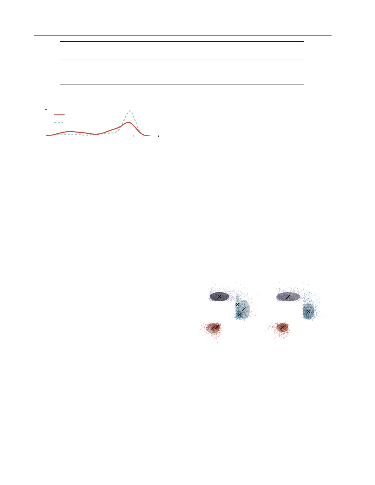
Rob ust Pr obabilistic Modeling with Bayesian Data Reweighting Y ixin W ang 1 Alp Kucukelbir 1 David M. Blei 1 Abstract Probabilistic models analyze data by relying on a set of assumptions. Data that exhibit de via- tions from these assumptions can undermine infer- ence and prediction quality . Robust models of fer protection against mismatch between a model’ s assumptions and reality . W e propose a way to systematically detect and mitigate mismatch of a large class of probabilistic models. The idea is to raise the likelihood of each observation to a weight and then to infer both the latent v ariables and the weights from data. Inferring the weights allo ws a model to identify observ ations that match its assumptions and down-weight others. This en- ables robust inference and impro ves predictive accuracy . W e study four dif ferent forms of mis- match with reality , ranging from missing latent groups to structure misspecification. A Poisson factorization analysis of the Movielens 1M dataset shows the benefits of this approach in a practical scenario. 1. Introduction Probabilistic modeling is a powerful approach to discov- ering hidden patterns in data. W e begin by expressing as- sumptions about the class of patterns we expect to discover; this is how we design a probability model. W e follow by inferring the posterior of the model; this is ho w we discover the specific patterns manifest in an observed data set. Ad- vances in automated inference ( Hof fman and Gelman , 2014 ; Mansinghka et al. , 2014 ; Kucukelbir et al. , 2017 ) enable easy de velopment of ne w models for machine learning and artificial intelligence ( Ghahramani , 2015 ). In this paper , we present a recipe to rob ustify probabilistic models. What do we mean by “robustify”? Departure from a model’ s assumptions can undermine its inference and prediction performance. This can arise due to corrupted 1 Columbia Univ ersity , New Y ork City , USA. Correspondence to: Y ixin W ang . Pr oceedings of the 34 th International Conference on Machine Learning , Sydney , Australia, PMLR 70, 2017. Copyright 2017 by the author(s). observat ions, or in general, measurements that do not belong to the process we are modeling. Robust models should perform well in spite of such mismatch with reality . Consider a movie recommendation system. W e gather data of people w atching movies via the account they use to log in. Imagine a situation where a few observ ations are corrupted For example, a child logs in to her account and regularly watches popular animated films. One day , her parents use the same account to watch a horror movie. Recommenda- tion models, like Poisson f actorization ( P F ), struggle with this kind of corrupted data (see Section 4 ): it be gins to recommend horror movies. What can be done to detect and mitigate this effect? One strategy is to design new models that are less sensitiv e to corrupted data, such as by replacing a Gaussian likelihood with a heavier -tailed t distribution ( Huber , 2011 ; Insua and Ruggeri , 2012 ). Most probabilistic models we use have more sophisticated structures; these template solutions for specific distributions are not readily applicable. Other clas- sical robust techniques act mostly on distances between observations ( Huber , 1973 ); these approaches struggle with high-dimensional data. How can we still make use of our fa- vorite probabilistic models while making them less sensitive to the messy nature of reality? Main idea. W e propose reweighted probabilistic models ( R P M ). The idea is simple. First, posit a probabilistic model. Then adjust the contribution of each observ ation by raising each likelihood term to its own (latent) weight. Finally , infer these weights along with the latent variables of the original probability model. The posterior of this adjusted model identifies observations that match its assumptions; it do wn- weights observations that disagree with its assumptions. 0 1 2 Density Uncorrupted Corrupted Original Model Reweighted Model Figure 1. Fitting a unimodal distrib ution to a dataset with corrupted measurements. The R P M do wnweights the corrupted observations. Figure 1 depicts this tradeof f. The dataset includes cor- Robust Pr obabilistic Modeling with Bayesian Data Reweighting rupted measurements that undermine the original model; Bayesian data re weighting automatically trades off the low likelihood of the corrupted data near 1.5 to focus on the uncorrupted data near zero. The R P M (green curve) detects this mismatch and mitigates its effect compared to the poor fit of the original model (red curve). Formally , consider a dataset of N independent observations y = ( y 1 , . . . , y N ) . The likelihood factorizes as a product Q N n =1 ` ( y n | β ) , where β is a set of latent variables. Posit a prior distribution p β ( β ) . Bayesian data reweighting follo ws three steps: 1. Define a probabilistic model p β ( β ) Q N n =1 ` ( y n | β ) . 2. Raise each likelihood to a positiv e latent weight w n . Then choose a prior on the weights p w ( w ) , where w = ( w 1 , . . . , w N ) . This gives a reweighted probabilistic model ( R P M ) p ( y , β , w ) = 1 Z p β ( β ) p w ( w ) N Y n =1 ` ( y n | β ) w n , where Z is the normalizing factor . 3. Infer the posterior of both the latent variables β and the weights w , p ( β , w | y ) . The latent weights w allo w an R P M to automatically explore which observ ations match its assumptions and which do not. Writing out the logarithm of the R P M gi ves some intuition; it is equal (up to an additiv e constant) to log p β ( β ) + log p w ( w ) + X n w n log ` ( y n | β ) . (1) Posterior inference, loosely speaking, seeks to maximize the abov e with respect to β and w . The prior on the weights p w ( w ) plays a critical role: it trades off extremely lo w likelihood terms, caused by corrupted measurements, while encouraging the weights to be close to one. W e study three options for this prior in Section 2 . How does Bayesian data reweighting induce robustness? First, consider ho w the weights w affect Equation (1) . The logarithm of our priors are dominated by the log w n term: this is the price of moving w n from one towards zero. By shrinking w n , we gain an increase in w n log ` ( y n | β ) while paying a price in a log w n . The gain outweighs the price we pay if log ` ( y n | β ) is very negati v e. Our priors are set to prefer w n to stay close to one; an R P M only shrinks w n for very unlikely (e.g., corrupted) measurements. Now consider ho w the latent v ariables β af fect Equation (1) . As the weights of unlikely measurements shrink, the like- lihood term can afford to assign low mass to those cor - rupted measurements and focus on the rest of the dataset. Jointly , the weights and latent variables work together to automatically identify unlikely measurements and focus on observations that match the original model’ s assumptions. Section 2 presents these intuitions in full detail, along with theoretical corroboration. In Section 3 , we study four mod- els under various forms of mismatch with reality , including missing modeling assumptions, misspecified nonlinearities, and ske wed data. R P M s provide better parameter inference and improved predicti v e accuracy across these models. Sec- tion 4 presents a recommendation system example, where we improv e on predictiv e performance and identify atypical film enthusiasts in the Movielens 1M dataset. Related work. Jerzy Neyman elegantly moti v ates the main idea behind robust probabilistic modeling, a field that has attracted much research attention in the past century . Every attempt to use mathematics to study some real phenomena must begin with b uilding a mathematical model of these phenomena. Of ne- cessity , the model simplifies matters to a greater or lesser extent and a number of details are ig- nored. [...] The solution of the mathematical problem may be correct and yet it may be in vi- olent conflict with realities simply because the original assumptions of the mathematical model di ver ge essentially from the conditions of the prac- tical problem considered. ( Neyman , 1949 , p.22). Our work draws on three themes around rob ust modeling. The first is a body of work on robust statistics and machine learning ( Prov ost and Fa wcett , 2001 ; Song et al. , 2002 ; Y u et al. , 2012 ; McW illiams et al. , 2014 ; Feng et al. , 2014 ; Shafieezadeh-Abadeh et al. , 2015 ). These dev elopments focus on making specific models more rob ust to imprecise measurements. One strategy is popular: localization. T o localize a proba- bilistic model, allo w each likelihood to depend on its o wn “copy” of the latent v ariable β n . This transforms the model into p ( y , β , α ) = p α ( α ) N Y n =1 ` ( y n | β n ) p β ( β n | α ) , (2) where a top-level latent variable α ties together all the β n variables ( de Finetti , 1961 ; W ang and Blei , 2015 ). 1 Lo- calization decreases the ef fect of imprecise measurements. R P M s present a broader approach to mitigating mismatch, with improved performance over localization ( Sections 3 and 4 ). 1 Localization also relates to James-Stein shrinkage; Efron ( 2010 ) connects these dots. Robust Pr obabilistic Modeling with Bayesian Data Reweighting The second theme is rob ust Bayesian analysis, which studies sensitivity with respect to the prior ( Berger et al. , 1994 ). Recent advances directly focus on sensitivity of the posterior ( Minsker et al. , 2014 ; Miller and Dunson , 2015 ) or the posterior predicti ve distribution ( Kucukelbir and Blei , 2015 ). W e draw connections to these ideas throughout this paper . The third theme is data reweighting. This inv olv es de- signing indi vidual re weighting schemes for specific tasks and models. Consider robust methods that toss away “out- liers. ” This strate gy in volv es manually assigning binary weights to datapoints ( Huber , 2011 ). Another example is cov ariate shift adaptation/importance sampling where reweighting transforms data to match another tar get distri- bution ( V each and Guibas , 1995 ; Sugiyama et al. , 2007 ; Shimodaira , 2000 ; W en et al. , 2014 ). A final example is maximum L q -likelihood estimation ( Ferrari et al. , 2010 ; Qin and Priebe , 2013 ; 2016 ). Its solutions can be interpreted as a solution to a weighted likelihood, whose weights are propor - tional to a po wer transformation of the density . In contrast, R P M s treat weights as latent variables. The weights are auto- matically inferred; no custom design is required. R P M s also closely connect to ideas around boosting ( Schapire and Fre- und , 2012 ) and v ariational tempering ( Mandt et al. , 2016 ), which also places an e xponential weight on the lik elihood term. Howe ver , they serve different purposes. Boosting reweights to b uild an ensemble of predictors for supervised learning; v ariational tempering reweights to escape poor local minima; R P M s reweight to mitigate model mismatch in Bayesian modeling. 2. Reweighted Probabilistic Models Reweighted probabilistic models ( R P M ) offer a ne w ap- proach to robust modeling. The idea is to automatically identify observations that match the assumptions of the model and to base posterior inference on these observ ations. 2.1. Definitions An R P M scaffolds ov er a probabilistic model, p β ( β ) Q N n =1 ` ( y n | β ) . Raise each likelihood to a la- tent weight and posit a prior on the weights. This gives the reweighted joint density p ( y , β , w ) = 1 Z p β ( β ) p w ( w ) N Y n =1 ` ( y n | β ) w n , (3) where Z = R p β ( β ) p w ( w ) Q N n =1 ` ( y n | β ) w n d y d β d w is the normalizing factor . The re weighted density inte grates to one when the normaliz- ing factor Z is finite. This is always true when the likelihood ` ( · | β ) is an exponential family distrib ution with Lesbegue base measure ( Bernardo and Smith , 2009 ); this is the class of models we study in this paper . 2 R P M s apply to likelihoods that f actorize ov er the observ a- tions. (W e discuss non-exchangeable models in Section 5 .) Figure 2 depicts an R P M as a graphical model. Specific models may hav e additional structure, such as a separation of local and global latent variables ( Hof fman et al. , 2013 ), or fixed parameters; we omit these in this figure. β y n p β N (a) Original probabilistic model β y n p β w n p w N (b) Reweighted probabilistic model ( R P M ) β n y n α p α N (c) Localized probabilistic model Figure 2. R P M s begin with a probabilistic model (a) and introduce a set of weights w as latent v ariables. This gi ves a model (b) that explores which data observations match its assumptions. Localiza- tion (c) , instead, builds a hierarchical model. ( Appendix A shows when a localized model is also an R P M .) The reweighted model introduces a set of weights; these are latent v ariables, each with support w n ∈ R > 0 . T o gain intuition, consider how these weights aff ect the posterior , which is proportional to the product of the likelihood of ev- ery measurement. A weight w n that is close to zero flattens out its corresponding likelihood ` ( y n | β ) w n ; a weight that is lar ger than one mak es its lik elihood more peaked. This, in turn, enables the posterior to focus on some measurements more than others. The prior p w ( w ) ensures that not too many likelihood terms get flattened; in this sense, it plays an important regularization role. W e study three options for this prior on weights: a bank of Beta distrib utions, a scaled Dirichlet distrib ution, and a bank of Gamma distributions. 2 Heavy-tailed lik elihoods and Bayesian nonparametric priors may violate this condition; we leav e these for future analysis. Robust Pr obabilistic Modeling with Bayesian Data Reweighting Bank of Beta priors. This option constrains each weight as w n ∈ (0 , 1) . W e posit an independent prior for each weight p w ( w ) = N Y n =1 Beta ( w n ; a, b ) (4) and use the same parameters a and b for all weights. This is the most conservati v e option for the R P M ; it ensures that none of the likelihoods e ver becomes more peaked than it was in the original model. The parameters a , b offer an expressi v e language to describe different attitudes to wards the weights. For e xample, setting both parameters less than one mak es the Beta act like a “tw o spikes and a slab” prior , encouraging weights to be close to zero or one, b ut not in between. As another example, setting a greater than b encourages weights to lean to wards one. Scaled Dirichlet prior . This option ensures the sum of the weights equals N . W e posit a symmetric Dirichlet prior on all the weights w = N v p v ( v ) = Dirichlet ( a 1 ) (5) where a is a scalar parameter and 1 is a ( N × 1) vector of ones. In the original model, where all the weights are one, then the sum of the weights is N . The Dirichlet option main- tains this balance; while certain likelihoods may become more peaked, others will flatten to compensate. The concentration parameter a giv es an intuitiv e way to configure the Dirichlet. Small values for a allow the model to easily up- or do wn-weight man y data observ ations; lar ger values for a prefer a smoother distribution of weights. The Dirichlet option connects to the bootstrap approaches in Rubin et al. ( 1981 ); Kucukelbir and Blei ( 2015 ), which also preserves the sum of weights as N . Bank of Gamma priors. Here we posit an independent Gamma prior for each weight p w ( w ) = N Y n =1 Gamma ( w n ; a, b ) (6) and use the same parameters a and b for all weights. W e do not recommend this option, because observations can be arbitrarily up- or down-weighted. In this paper , we only consider Equation (6) for our theoretical analysis in Sec- tion 2.2 . The bank of Beta and Dirichlet options perform similarly . W e prefer the Beta option as it is more conservati v e, yet find the Dirichlet to be less sensiti v e to its parameters. W e explore these options in the empirical study ( Section 3 ). 2.2. Theory and intuition How can theory justify Bayesian data re weighting? Here we in v estigate its robustness properties. These analyses intend to confirm our intuition from Section 1 . Appendices B and C present proofs in full technical detail. Intuition . Recall the logarithm of the R P M joint density from Equation (1) . Now compute the maximum-a-posterior ( M A P ) estimate of the weights w . The partial deriv ati v e is ∂ log p ( y , β , w ) ∂ w n = d log p w ( w n ) d w n + log ` ( y n | β ) (7) for all n = 1 , . . . , N . Plug the Gamma prior from Equa- tion (6) into the partial deri v ativ e in Equation (7) and set it equal to zero. This gives the M A P estimate of w n , b w n = a − 1 b − log ` ( y n | β ) . (8) The M A P estimate b w n is an increasing function of the log likelihood of y n when a > 1 .This reveals that b w n shrinks the contribution of observ ations that are unlik ely under the log likelihood; in turn, this encourages the M A P estimate for b β to describe the majority of the observations. This is how an R P M makes a probabilistic model more rob ust. A similar ar gument holds for other exponential family priors on w with log w n as a sufficient statistic. W e formalize this intuition and generalize it in the follo wing theorem, which establishes sufficient conditions where a R P M improves the inference of its latent variables β . Theorem 1 Denote the true value of β as β ∗ . Let the pos- terior mean of β under the weighted and unweighted model be ¯ β w and ¯ β u r espectively . Assume mild conditions on p w , ` and the corruption level, and that | ` ( y n | ¯ β w ) − ` ( y n | β ∗ ) | <  holds ∀ n with high pr obability . Then, ther e exists an N ∗ such that for N > N ∗ , we have | ¯ β u − β ∗ |  2 | ¯ β w − β ∗ | , wher e  2 denotes second or der stochastic dominance . (Details in Appendix B .) The likelihood bounding assumption is common in rob ust statistics theory; it is satisfied for both likely and unlikely (corrupted) measurements. How much of an improv ement does it giv e? W e can quantify this through the influence function ( I F ) of ¯ β w . Consider a distribution G and a statistic T ( G ) to be a func- tion of data that comes iid from G . T ake a fixed distrib ution, e.g., the population distribution, F . Then, I F ( z ; T , F ) mea- sures how much an additional observation at z affects the statistic T ( F ) . Define I F ( z ; T , F ) = lim t → 0 + T ( tδ z + (1 − t ) F ) − T ( F ) t Robust Pr obabilistic Modeling with Bayesian Data Reweighting for z where this limit e xists. Roughly , the I F measures the asymptotic bias on T ( F ) caused by a specific observation z that does not come from F . W e consider a statistic T to be robust if its I F is a bounded function of z , i.e., if outliers can only ex ert a limited influence ( Huber , 2011 ). Here, we study the I F of the posterior mean T = ¯ β w under the true data generating distribution F = ` ( · | β ∗ ) . Say a val ue z has likelihood ` ( z | β ∗ ) that is nearly zero; we think of this z as corrupted. Now consider the weight function induced by the prior p w ( w ) . Rewrite it as a function of the log likelihood, like w (log ` ( · | β ∗ )) as in Equation (8) . Theorem 2 If lim a →−∞ w ( a ) = 0 and lim a →−∞ a · w ( a ) < ∞ , then I F ( z ; ¯ β w , ` ( · | β ∗ )) → 0 as ` ( z | β ∗ ) → 0 . This result shows that an R P M is robust in that its I F goes to zero for unlikely measurements. This is true for all three priors. (Details in Appendix C .) 2.3. Inference and computation W e now turn to inferring the posterior of an R P M , p ( β , w | y ) . The posterior lacks an analytic closed-form expression for all but the simplest of models; ev en if the original model admits such a posterior for β , the re weighted posterior may take a dif ferent form. T o approximate the posterior , we appeal to probabilistic pro- gramming. A probabilistic programming system enables a user to write a probability model as a computer program and then compile that program into an inference ex ecutable. Au- tomated inference is the backbone of such systems: it takes in a probability model, expressed as a program, and outputs an ef ficient algorithm for inference. W e use automated infer- ence in Stan, a probabilistic programming system ( Carpenter et al. , 2015 ). In the empirical study that follows, we highlight how R P M s detect and mitigate various forms of model mismatch. As a common metric, we compare the predicti ve accurac y on held out data for the original, localized, and reweighted model. The posterior predictiv e likelihood of a new datapoint y † is p original ( y † | y ) = R ` ( y † | β ) p ( β | y ) d β . Lo- calization couples each observation with its o wn copy of the latent variable; this giv es p localized ( y † | y ) = R R ` ( y † | β † ) p ( β † | α ) p ( α | y ) d α d β † where β † is the lo- calized latent variable for the ne w datapoint. The prior p ( β † | α ) has the same form as p β in Equation (2) . Bayesian data reweighting gi v es the following posterior predictiv e likelihood p R P M ( y † | y ) = Z Z p ( y † | β , w † ) p R P M ( β | y ) p ( w † ) d w † d β , where p R P M ( β | y ) is the marginal posterior , integrating out the inferred weights of the training dataset, and the prior p ( w † ) has the same form as p w in Equation (3) . 3. Empirical Study W e study R P M s under four types of mismatch with reality . This section in v olves simulations of realistic scenarios; the next section presents a recommendation system example using real data. W e default to No-U-T urn sampler ( N U T S ) ( Hoffman and Gelman , 2014 ) for inference in all experi- ments, e xcept for Sections 3.5 and 4 where we le verage vari- ational inference ( Kucuk elbir et al. , 2017 ). The additional computational cost of inferring the weights is unnoticeable relativ e to inference in the original model. 3.1. Outliers: a network wait-time example A router receiv es packets o ver a netw ork and measures the time it waits for each packet. Suppose we typically observe wait-times that follo w a Poisson distribution with rate β = 5 . W e model each measurement using a Poisson likelihood ` ( y n | β ) = Poisson ( β ) and posit a Gamma prior on the rate p β ( β ) = Gam ( a = 2 , b = 0 . 5) . Imagine that F % percent of the time, the network fails. During these failures, the w ait-times come from a Poisson with much higher rate β = 50 . Thus, the data actually contains a mixture of two Poisson distributions; yet, our model only assumes one. (Details in Appendix D.1 .) 0 5 10 15 20 β Density truth prior original R P M Beta R P M Dirichlet localized (a) Posteriors for F = 25% failure rate. 0 0 . 1 0 . 2 0 . 3 0 . 4 5 15 25 F β original R P M Beta R P M Dirichlet localized (b) Posterior 95% credible intervals. Figure 3. Outliers simulation study . W e compare Beta (0 . 1 , 0 . 01) and Dir ( 1 ) as priors for the reweighted probabilistic model. (a) Posterior distributions on β show a marked dif ference in detecting the correct wait-time rate of β = 5 . (b) Posterior 95% confidence intervals across failure rates F show consistent behavior for both Beta and Dirichlet priors. ( N = 100 with 50 replications.) Robust Pr obabilistic Modeling with Bayesian Data Reweighting How do we e xpect an R P M to behav e in this situation? Suppose the network failed 25% of the time. Figure 3a shows the posterior distribution on the rate β . The original posterior is centered at 18; this is troubling, not only because the rate is wrong but also because of ho w confident the posterior fit is. Localization introduces greater uncertainty , yet still estimates a rate around 15. The R P M correctly identifies that the majority of the observations come from β = 5 . Observations from when the netw ork failed are down-weighted. It gives a confident posterior centered at fiv e. Figure 3b shows posterior 95% credible interv als of β under failure rates up to F = 45% . The R P M is rob ust to corrupted measurements; instead it focuses on data that it can explain within its assumptions. When there is no corruption, the R P M performs just as well as the original model. V isualizing the weights elucidates this point. Figure 4 sho ws the posterior mean estimates of w for F = 25% . The weights are sorted into two groups, for ease of viewing. The weights of the corrupted observations are essentially zero; this downweighting is what allows the R P M to shift its posterior on β towards fi v e. 0 75 100 0 1 2 Data Index W eights Figure 4. Posterior means of the weights w under the Dirichlet prior . For visualization purposes, we sorted the data into two groups: the first 75 contain observations from the normal network; the remaining 25 are the observations when the netw ork fails. Despite this downweighting, the R P M posteriors on β are not o verdispersed, as in the localized case. This is due to the interplay we described in the introduction. Downweighting observations should lead to a smaller effecti ve sample size, which would increase posterior uncertainty . But the do wn- weighted datapoints are corrupted observ ations; including them also increases posterior uncertainty . The R P M is insensitiv e to the prior on the weights; both Beta and Dirichlet options perform similarly . From here on, we focus on the Beta option. W e let the shape parameter a scale with the data size N such that N /a ≈ 10 3 ; this encodes a mild attitude to wards unit weights. W e now mov e on to other forms of mismatch with reality . 3.2. Missing latent groups: predicting color blindness Color blindness is une venly hereditary: it is much higher for men than for women ( Boron and Boulpaep , 2012 ). Suppose we are not aware of this fact. W e have a dataset of both gen- ders with each indi vidual’ s color blindness status and his/her relev ant family history . No gender information is av ailable. Consider analyzing this data using logistic regression. It can only capture one hereditary group. Thus, logistic regression misrepresents both groups, ev en though men exhibit strong heredity . In contrast, an R P M can detect and mitigate the missing group effect by focusing on the dominant hereditary trait. Here we consider men as the dominant group. W e simulate this scenario by drawing binary indicators of color blindness y n ∼ Bernoulli (1 / 1 + exp ( − p n )) where the p n ’ s come from tw o latent groups: men exhibit a stronger dependency on f amily history ( p n = 0 . 5 x n ) than women ( p n = 0 . 01 x n ). W e simulate family history as x n ∼ Unif ( − 10 , 10) . Consider a Bayesian logistic regres- sion model without intercept. Posit a prior on the slope as p β ( β ) = N (0 , 10) and assume a Beta (0 . 1 , 0 . 01) prior on the weights. (Details in Appendix D.2 .) 0 0.1 0.2 0.3 0.4 0 . 5 1 F β β men original R P M localized Figure 5. Missing latent groups study . Posterior 95% credible intervals for the R P M always include the dominant β men = 0 . 5 , as we vary the percentage of females in the data. Dataset size N = 100 with 50 replications. Figure 5 shows the posterior 95% credible intervals of β as we v ary the percentage of females from F = 0% to 40%. A horizontal line indicates the correct slope for the dominant group, β men = 0 . 5 . As the size of the missing latent group (women) increases, the original model quickly shifts its credible interval away from 0 . 5 . The reweighted and localized posteriors both contain β men = 0 . 5 for all percentages, but the localized model exhibits much higher variance in its estimates. This analysis shows how R P M s can mitigate the effect of missing latent groups. While the original logistic regression model would perform equally poorly on both groups, an R P M is able to automatically focus on the dominant group. An R P M also functions as a diagnostic tool to detect mis- match with reality . The distribution of the inferred weights indicates the presence of datapoints that defy the assump- tions of the original model. Figure 6 shows a kernel density estimate of the inferred posterior weights. A hypothetical dataset with no corrupted measurements receives weights close to one. In contrast, the actual dataset with measure- ments from a missing latent group exhibit a bimodal dis- Robust Pr obabilistic Modeling with Bayesian Data Reweighting T rue structure Model structure Original R P M Localization mean(std) mean(std) mean(std) β 0 + β 1 x 1 + β 2 x 2 + β 3 x 1 x 2 β 0 + β 1 x 1 + β 2 x 2 3.16(1.37) 2.20 (1.25) 2.63(1.85) β 0 + β 1 x 1 + β 2 x 2 + β 3 x 2 2 β 0 + β 1 x 1 + β 2 x 2 30.79(2.60) 16.32 (1.96) 21.08(5.20) β 0 + β 1 x 1 + β 2 x 2 β 0 + β 1 x 1 0.58 (0.38) 0.60(0.40) 0.98(0.54) T able 1. R P M s improve absolute de viations of posterior mean β 1 estimates. (50 replications.) 0 1 E p ( w | y ) [ w ] Density Corrupted ( F = 25% ) Clean ( F = 0% ) Figure 6. Kernel density estimate of the distribution of weights across all measurements in the missing latent groups study . The percentage of females is denoted by F . A hypothetical clean dataset receiv es weights that concentrate around one; the actual corrupted dataset exhibits a two-hump distrib ution of weights. tribution of weights. T esting for bimodality of the inferred weights is one way in which an R P M can be used to diagnose mismatch with reality . 3.3. Covariate dependence misspecification: a lung cancer risk study Consider a study of lung cancer risk. While tobacco usage exhibits a clear connection, other factors may also contribute. For instance, obesity and tobacco usage appear to interact, with evidence towards a quadratic dependence on obesity ( Odegaard et al. , 2010 ). Denote tobacco usage as x 1 and obesity as x 2 . W e study three models of lung cancer risk dependency on these co- variates. W e are primarily interested in understanding the effect of tobacco usage; thus we focus on β 1 , the regression coefficient for tobacco. In each model, some form of cov ari- ance misspecification discriminates the true structure from the assumed structure. For each model, we simulate a dataset of size N = 100 with random cov ariates x 1 ∼ N (10 , 5 2 ) and x 2 ∼ N (0 , 10 2 ) and regression coef ficients β 0 , 1 , 2 , 3 ∼ Unif ( − 10 , 10) . Con- sider a Bayesian linear re gression model with prior p β ( β ) = N (0 , 10) . (Details in Appendix D.3 .) T able 1 summarizes the misspecification and shows absolute differences on the estimated β 1 regression coef ficient. The R P M yields better estimates of β 1 in the first two models. These highlight ho w the R P M lev erages datapoints useful for estimating β 1 . The third model is particularly challenging because obesity is ignored in the misspecified model. Here, the R P M gi ves similar results to the original model; this highlights that R P M s can only use av ailable information. Since the original model lacks dependence on x 2 , the R P M cannot compensate for this. 3.4. Predicti ve likelihood r esults T able 2 sho ws how R P M s also improve predicti v e accuracy . In all the abov e examples, we simulate test data with and without their respectiv e types of corruption. R P M s improve prediction for both clean and corrupted data, as the y focus on data that match the assumptions of the original model. 3.5. Skewed data: cluster selection in a mixture model Finally , we show how R P M s handle ske wed data. The Dirichlet process mixture model ( D P M M ) is a versatile model for density estimation and clustering ( Bishop , 2006 ; Murphy , 2012 ). While real data may indeed come from a finite mixture of clusters, there is no reason to assume each cluster is distributed as a Gaussian. Inspired by the experiments in Miller and Dunson ( 2015 ), we sho w ho w a reweighted D P M M reliably recovers the correct number of components in a mixture of ske wnormals dataset. (a) Original model (b) R P M Figure 7. A finite approximation D P M M to ske wnormal distributed data that come from three groups. The shade of each cluster indicates the inferred mixture proportions ( N = 2000 ). A standard Gaussian mixture model ( G M M ) with large K and a sparse Dirichlet prior on the mixture proportions is an approximation to a D P M M ( Ishwaran and James , 2012 ). W e simulate three clusters from tw o-dimensional ske wnor - mal distributions and fit a G M M with maximum K = 30 . Here we use automatic differentiation v ariational inference ( A DV I ), as N U T S struggles with inference of mixture mod- els ( Kucukelbir et al. , 2017 ). (Details in Appendix D.4 .) Robust Pr obabilistic Modeling with Bayesian Data Reweighting Outliers Missing latent groups Misspecified structur e Clean Corrupted Clean Corrupted Clean Corrupted Original model −744.2 −1244.5 −108.6 −103.9 −136.3 −161.7 Localized model −730.8 −1258.4 −53.6 −112.7 −192.5 −193.1 R P M −328.5 −1146.9 −43.9 −90.5 −124.1 −144.1 T able 2. Posterior predictiv e likelihoods of clean and corrupted test data. Outliers and missing latent groups hav e F = 25% . The misspecified structure is missing the interaction term. Results are similar for other le vels and types of mismatch with reality . A verage log likelihood Corrupted users 0% 1% 2% Original model − 1 . 68 − 1 . 73 − 1 . 74 R P M − 1 . 53 − 1 . 53 − 1 . 52 T able 3. Held-out predictiv e accuracy under varying amounts of corruption. Held-out users chosen randomly ( 20% of total users). Figure 7 sho ws posterior mean estimates from the original G M M ; it incorrectly finds six clusters. In contrast, the R P M identifies the correct three clusters. Datapoints in the tails of each cluster get down-weighted; these are datapoints that do not match the Gaussianity assumption of the model. 4. Case Study: P oisson factorization f or recommendation W e now turn to a study of real data: a recommendation system. Consider a video streaming service; data comes as a binary matrix of users and the movies they choose to watch. How can we identify patterns from such data? Poisson factorization ( P F ) offers a fle xible solution ( Cemgil , 2009 ; Gopalan et al. , 2015 ). The idea is to infer a K -dimensional latent space of user preferences θ and movie attributes β . The inner product θ > β determines the rate of a Poisson likelihood for each binary measurement; Gamma priors on θ and β promote sparse patterns. As a result, P F finds interpretable groupings of movies, often clustered according to popularity or genre. (Full model in Appendix E .) How does classical P F compare to its re weighted counter- part? As input, we use the MovieLens 1M dataset, which contains one million movie ratings from 6 000 users on 4 000 movies. W e place iid Gamma (1 , 0 . 001) priors on the preferences and attrib utes. Here, we hav e the option of reweighting users or items. W e focus on users and place a Beta (100 , 1) prior on their weights. For this model, we use M A P estimation. (Localization is computationally challeng- ing for P F ; it requires a separate “copy” of θ for each movie, along with a separate β for each user . This dramatically increases computational cost.) W e begin by analyzing the original (clean) dataset. clean 0 . 5 1 W eights (a) Original dataset 0.1 0.5 1 0 . 5 1 Ratio of corruption ( R ) (b) Corrupted users Figure 8. Inferred weights for clean and corrupted data. (a) Most users recei ve weights v ery close to one. (b) Corrupted users recei ve weights much smaller than one. Larger ratios of corruption R imply lower weights. Reweighting improves the av erage held-out log lik elihood from − 1 . 68 of the original model to − 1 . 53 of the corre- sponding R P M . The boxplot in Figure 8a sho ws the inferred weights. The majority of users recei ve weight one, b ut a fe w users are do wn-weighted. These are film enthusiasts who appear to indiscriminately watch man y movies from man y genres. ( Appendix F shows an example.) These users do not contribute to w ards identifying movies that go together; this explains why the R P M down-weights them. Recall the example from our introduction. A child typically watches popular animated films, but her parents occasionally use her account to watch horror films. W e simulate this by corrupting a small percentage of users. W e replace a ratio R = (0 . 1 , 0 . 5 , 1) of these users’ movies with randomly selected movies. The boxplot in Figure 8b shows the weights we infer for these corrupted users, based on ho w many of their mo vies we randomly replace. The weights decrease as we corrupt more movies. T able 3 sho ws ho w this leads to higher held- out predictive accuracy; down-weighting these corrupted users leads to better prediction. 5. Discussion Reweighted probabilistic models ( R P M ) offer a systematic approach to mitigating v arious forms of mismatch with reality . The idea is to raise each data likelihood to a weight and to infer the weights along with the hidden patterns. W e demonstrate ho w this strate gy introduces rob ustness and Robust Pr obabilistic Modeling with Bayesian Data Reweighting improv es prediction accuracy across four types of mismatch. R P M s also offer a way to detect mismatch with reality . The distribution of the inferred weights sheds light onto data- points that fail to match the original model’ s assumptions. R P M s can thus lead to new model de velopment and deeper insights about our data. R P M s can also work with non-exchangeable data, such as time series. Some time series models admit exchange- able likelihood approximations ( Guinness and Stein , 2013 ). For other models, a non-ov erlapping windo wing approach would also work. The idea of reweighting could also e xtend to structured likelihoods, such as Hawk es process models. Acknowledgements W e thank Adji Dieng, Y uanjun Gao, Inchi Hu, Christian Naesseth, Rajesh Ranganath, Francisco Ruiz, Dustin T ran, and Joshua V ogelstein for their insightful pointers and com- ments. This work is supported by NSF IIS-1247664, ONR N00014-11-1-0651, D ARP A PP AML F A8750-14-2-0009, D ARP A SIMPLEX N66001-15-C-4032, and the Alfred P . Sloan Foundation. References Berger , J. O., Moreno, E., Pericchi, L. R., Bayarri, M. J., Bernardo, J. M., Cano, J. A., De la Horra, J., Martín, J., Ríos-Insúa, D., Betrò, B., et al. (1994). An overvie w of robust Bayesian analysis. T est , 3(1):5–124. Bernardo, J. M. and Smith, A. F . (2009). Bayesian Theory . John W ile y & Sons. Bishop, C. M. (2006). P attern Recognition and Machine Learning . Springer New Y ork. Boron, W . F . and Boulpaep, E. L. (2012). Medical Physiol- ogy . Elsevier . Carpenter , B., Gelman, A., Hof fman, M., Lee, D., Goodrich, B., Betancourt, M., Brubaker , M. A., Guo, J., Li, P ., and Riddell, A. (2015). Stan: a probabilistic programming language. Journal of Statistical Softwar e . Cemgil, A. T . (2009). Bayesian inference for nonnegati ve matrix factorisation models. Computational Intelligence and Neur oscience . de Finetti, B. (1961). The Bayesian approach to the rejec- tion of outliers. In Pr oceedings of the F ourth Berkele y Symposium on Pr obability and Statistics . Efron, B. (2010). Large-Scale Infer ence . Cambridge Uni- versity Press. Feng, J., Xu, H., Mannor, S., and Y an, S. (2014). Robust logistic regression and classification. In NIPS . Ferrari, D., Y ang, Y ., et al. (2010). Maximum lq-lik elihood estimation. The Annals of Statistics , 38(2):753–783. Ghahramani, Z. (2015). Probabilistic machine learning and artificial intelligence. Nature , 521(7553):452–459. Gopalan, P ., Hofman, J. M., and Blei, D. M. (2015). Scalable recommendation with hierarchical Poisson factorization. U AI . Guinness, J. and Stein, M. L. (2013). T ransformation to ap- proximate independence for locally stationary Gaussian processes. Journal of T ime Series Analysis , 34(5):574– 590. Hoffman, M. D., Blei, D. M., W ang, C., and P aisley , J. (2013). Stochastic variational inference. The Journal of Machine Learning Resear ch , 14(1):1303–1347. Hoffman, M. D. and Gelman, A. (2014). The No-U- Turn sampler . Journal of Machine Learning Researc h , 15(1):1593–1623. Huber , P . J. (1973). Rob ust re gression: asymptotics, conjec- tures and Monte Carlo. The Annals of Statistics , pages 799–821. Huber , P . J. (2011). Robust Statistics . Springer . Insua, D. R. and Ruggeri, F . (2012). Rob ust Bayesian Anal- ysis . Springer Science & Business Media. Ishwaran, H. and James, L. F . (2012). Approximate Dirichlet process computing in finite normal mixtures. Journal of Computational and Graphical Statistics . Kucukelbir , A. and Blei, D. M. (2015). Population empirical Bayes. In UAI . Kucukelbir , A., Tran, D., Ranganath, R., Gelman, A., and Blei, D. M. (2017). Automatic dif ferentiation v aria- tional inference. Journal of Machine Learning Resear ch , 18(14):1–45. Mandt, S., McInerney , J., Abrol, F ., Ranganath, R., and Blei, D. (2016). V ariational tempering. In Artificial Intelligence and Statistics , pages 704–712. Mansinghka, V ., Selsam, D., and Perov , Y . (2014). V enture: a higher-order probabilistic programming platform with programmable inference. . McW illiams, B., Krummenacher , G., Lucic, M., and Buh- mann, J. M. (2014). F ast and robust least squares estima- tion in corrupted linear models. In NIPS . Miller , J. W . and Dunson, D. B. (2015). Robust Bayesian in- ference via coarsening. arXiv preprint . Robust Pr obabilistic Modeling with Bayesian Data Reweighting Minsker , S., Sri v astav a, S., Lin, L., and Dunson, D. B. (2014). Robust and scalable Bayes via a median of subset posterior measures. arXiv preprint . Murphy , K. P . (2012). Mac hine Learning: a Pr obabilistic P erspective . MIT Press. Neyman, J. (1949). On the problem of estimating the number of schools of fish. In J. Neyman, M. L. and Y erushalmy , J., editors, University of California Publi- cations in Statistics , volume 1, chapter 3, pages 21–36. Univ ersity of California Press. Odegaard, A. O., Pereira, M. A., K oh, W .-P ., Gross, M. D., Duval, S., Mimi, C. Y ., and Y uan, J.-M. (2010). BMI, all-cause and cause-specific mortality in Chinese Singa- porean men and women. PLoS One , 5(11). Prov ost, F . and Fa wcett, T . (2001). Rob ust classification for imprecise en vironments. Machine Learning , 42(3):203– 231. Qin, Y . and Priebe, C. E. (2013). Maximum l q-likelihood estimation via the e xpectation-maximization algorithm: A robust estimation of mixture models. Journal of the American Statistical Association , 108(503):914–928. Qin, Y . and Priebe, C. E. (2016). Robust hypothesis testing via lq-likelihood. Rubin, D. B. et al. (1981). The Bayesian bootstrap. The annals of statistics , 9(1):130–134. Schapire, R. and Freund, Y . (2012). Boosting: F oundations and Algorithms . MIT Press. Shafieezadeh-Abadeh, S., Esfahani, P . M., and Kuhn, D. (2015). Distributionally robust logistic regression. In NIPS . Shimodaira, H. (2000). Improving predictiv e inference under cov ariate shift by weighting the log-likelihood function. Journal of Statistical Planning and Infer ence , 90(2):227–244. Song, Q., Hu, W ., and Xie, W . (2002). Rob ust support v ector machine with b ullet hole image classification. Systems, Man, and Cybernetics, P art C: Applications and Reviews, IEEE T ransactions on , 32(4):440–448. Sugiyama, M., Krauledat, M., and Müller , K.-R. (2007). Cov ariate shift adaptation by importance weighted cross validat ion. J ournal of Machine Learning Resear c h , 8:985– 1005. V each, E. and Guibas, L. J. (1995). Optimally combin- ing sampling techniques for Monte Carlo rendering. In Pr oceedings of the 22nd annual confer ence on Com- puter graphics and interactive techniques , pages 419–428. A CM. W ang, C. and Blei, D. M. (2015). A general method for robust Bayesian modeling. arXiv pr eprint arXiv:1510.05078 . W en, J., Y u, C.-n., and Greiner, R. (2014). Robust learning under uncertain test distributions: Relating cov ariate shift to model misspecification. In ICML . Y u, Y ., Aslan, O., and Schuurmans, D. (2012). A polynomial-time form of robust re gression. In NIPS . Robust Pr obabilistic Modeling with Bayesian Data Reweighting A. Localized generalized linear model as an R P M Localization in generalized linear models ( G L M s ) is equiv alent to reweighting, with constraints on the weight function w ( · ) induced by p w . W e prelude the theorem with a simple illustration in linear regression. Consider N iid observations { ( x n , y n ) } N 1 . W e regress y against x : y n = β 1 ( x n − ¯ x ) + β 0 +  n ,  n iid ∼ N (0 , σ 2 ) , where ¯ x = P N n =1 x n . The maximum likelihood estimate of ( β 0 , β 1 ) is ( b β 0 , b β 1 ) = argmin β 0 ,β 1 N X n =1 ( y n − β 1 ( x n − ¯ x ) − β 0 ) 2 . The localized model is y n = β 1 n × ( x n − ¯ x ) + β 0 +  n , β 1 n iid ∼ N ( β 1 , λ 2 ) ,  n iid ∼ N (0 , σ 2 ) , where { β 1 n } N n =1 ⊥ ⊥ {  n } N n =1 . Marginalizing out β 1 n ’ s gives y n = β 1 × ( x n − ¯ x ) + β 0 + γ n , γ n iid ∼ N (0 , ( x n − ¯ x ) 2 · λ 2 + σ 2 ) . The maximum likelihood estimate of ( β 0 , β 1 ) in the localized model thus becomes ( b β 0 , b β 1 ) = argmin β 0 ,β 1 N X n =1 ( y n − β 1 ( x n − ¯ x ) − β 0 ) 2 ( x n − ¯ x ) 2 · λ 2 + σ 2 . This is equiv alent to the reweighting approach with w n = 1 ( x n − ¯ x ) 2 · λ 2 + σ 2 . W e generalize this argument into generalized linear models. Theorem 3 Localization in a G L M with identity link infers β 1 fr om y n | x n , β 1 n , β 0 ∼ exp  y n · η n − b 1 ( η n ) a 1 ( φ ) + c 1 ( y n , φ )  , η n = β 0 + β 1 n · ( x n − ¯ x ) , β 1 n | β 1 ∼ exp  β 1 n · β 1 − b 2 ( β 1 ) a 2 ( ν ) + c 2 ( β 1 n , ν )  , wher e a 1 ( · ) , a 2 ( · ) denote disper sion constants, b 1 ( · ) , b 2 ( · ) denote normalizing constants, and c 1 ( · ) , c 2 ( · ) denote carrier densities of exponential family distrib utions. Inferring β 1 fr om this localized G L M is equivalent to inferring β 1 fr om the r eweighted model with weights w n = E p ( β 1 n | β 1 ) " exp ( y n − E ( y n | β 0 + ˜ β 1 n ( x n − ¯ x )))( β 1 n − β 1 )( x n − ¯ x ) a 1 ( φ ) !# for some { ˜ β 1 n } N 1 . Proof A classical G L M with an identity link is y n ∼ exp  y n · η n − b 1 ( η n ) a 1 ( φ ) + c 1 ( y n , φ )  , Robust Pr obabilistic Modeling with Bayesian Data Reweighting η n = β 0 + β 1 · ( x n − ¯ x ) , whose maximum likelihood estimate calculates ( b β 0 , b β 1 ) = argmax β 0 ,β 1 N Y n =1 L c,n , where L c,n = exp  y n · ( β 0 + β 1 ( x n − ¯ x )) − b 1 ( β 0 + β 1 ( x n − ¯ x )) a 1 ( φ ) + c 1 ( y n , φ )  . On the other hand, the maximum likelihood estimate of the localized model calculates ( b β 0 , b β 1 ) = argmax β 0 ,β 1 N Y n =1 L l,n , where L l,n = Z exp  y n · ( β 0 + β 1 n ( x n − ¯ x )) − b 1 ( β 0 + β 1 n ( x n − ¯ x )) a 1 ( φ ) + c 1 ( y n , φ ) + β 1 n β 1 − b 2 ( β 1 ) a 2 ( ν ) + c 2 ( β 1 n , ν )  dβ 1 n . A localized G L M is thus reweighting the lik elihood term of each observation by L l,n L c,n = Z exp  y n ( β 1 n − β 1 )( x n − ¯ x ) − b 1 ( β 0 + β 1 n ( x n − ¯ x )) + b 1 ( β 0 + β 1 ( x n − ¯ x )) a 1 ( φ ) + β 1 n β 1 − b 2 ( β 1 ) a 2 ( ν ) + c 2 ( β 1 n , ν )  dβ 1 n = Z exp y n ( β 1 n − β 1 )( x n − ¯ x ) − b 0 1 ( β 0 + ˜ β 1 n ( x n − ¯ x ))( β 1 n − β 1 )( x n − ¯ x ) a 1 ( φ ) + β 1 n β 1 − b 2 ( β 1 ) a 2 ( ν ) + c 2 ( β 1 n , ν )  dβ 1 n = Z exp ( y n − b 0 1 ( β 0 + ˜ β 1 n ( x n − ¯ x )))( β 1 n − β 1 )( x n − ¯ x ) a 1 ( φ ) + β 1 n β 1 − b 2 ( β 1 ) a 2 ( ν ) + c 2 ( β 1 n , ν )) dβ 1 n = E p ( β 1 n | β 1 ) exp ( y n − E ( y n | β 0 + ˜ β 1 n ( x n − ¯ x )))( β 1 n − β 1 )( x n − ¯ x ) a 1 ( φ ) ! where ˜ β 1 n is some value between β 1 and β 1 n and the second equality is due to mean value theorem. The last equality is due to y n residing in the exponential family .  Robust Pr obabilistic Modeling with Bayesian Data Reweighting B. Proof sk etch of theor em 1 Denote as ` ( y | β : β ∈ Θ) the statistical model we fit to the data set y 1 , ..., y N iid ∼ ¯ P N . ` ( ·| β ) is a density function with respect to some carrier measure ν ( dy ) , and Θ is the parameter space of β . Denote the desired true value of β as β 0 . Let p 0 ( dβ ) be the prior measure absolute continuous in a neighborhood of β 0 with a continuous density at β 0 . Let p w ( dw ) be the prior measure on weights ( w n ) N n =1 . Finally , let the posterior mean of β under the weighted and unweighted model be ¯ β w and ¯ β u and the corresponding maximum likelihood estimate ( M L E ) be b β w and b β u respectiv ely . Let us start with some assumptions. Assumption 1 ` ( ·| β ) is twice-differ entiable and log-concave . Assumption 2 Ther e exist an incr easing function w ( · ) : R → R + such that w n = w (log ` ( y n | β )) solves ∂ ∂ w n p w (( w n ) N n =1 ) + log ` ( y n | β ) = 0 , n = 1 , ..., N . W e can immediately see that the bank of Beta ( α, β ) priors with α > 1 and the bank of Gamma ( k , θ ) priors with k > 1 satisfy this condition. Assumption 3 P ( | log ` ( y n | b β w ) − log ` ( y n | β 0 ) | <  ) > 1 − δ 1 holds ∀ n for some , δ 1 > 0 . This assumption includes the follo wing two cases: (1) b β w is close to the true parameter β 0 , i.e. the corruption is not at all influential in parameter estimation, and (2) deviant points in y 1 , ..., y N are far enough from typical observ ations coming from ` ( y | β 0 ) that log ` ( y n | b β w ) and log ` ( y n | β 0 ) almost coincide. This assumption precisely explains why the R P M performs well in Section 3 . Assumption 4 | b β u − β 0 | ≥ M for some M . Assumption 5 Ther e exist a permutation π ( i ) : { 1 , ..., N } → { 1 , ..., N } s.t. P ( k X n =1 log ` ( y π ( i ) | β 0 ) 0 P N n =1 log ` ( y π ( i ) | β 0 ) 0 ≤ (1 − 4  M ) k X n =1 log ` ( y π ( i ) | ˜ β n ) 00 P N n =1 log ` ( y π ( i ) | ˇ β n ) 00 , k = 1 , ..., n − 1) ≥ 1 − δ 2 , for ˜ β n and ˇ β n between b β u and β 0 and for some δ 2 > 0 . By noticing that P N n =1 log ` ( y n | β 0 ) 0 P N n =1 log ` ( y n | β 0 ) 0 = 1 , P N n =1 log ` ( y n | ˜ β n ) 00 P N n =1 log ` ( y n | ˇ β n ) 00 (1 − 4  M ) ≈ 1 , and V ar ( log ` ( y n | β ) 0 ) >> V ar (log ` ( y n | β ) 00 ) in general, this assumption is not particularly restrictiv e. For instance, a normal likelihood has V ar (log ` ( y n | β ) 00 ) = 0 . Theorem Assume Assumption 1 - Assumption 5 . There e xists an N ∗ such that for N > N ∗ , we have | ¯ β u − β 0 |  2 | ¯ β w − β 0 | , where  2 denotes second order stochastic dominance. Pr oof Sk etch. W e resort to M A P estimates of { w n } N 1 and δ 1 = δ 2 = 0 for simplicity of the sketch. By Bernstein-von Mises theorem, there exists N ∗ s.t. N > N ∗ implies the posterior means ¯ β w and ¯ β u are close to their corresponding M L E s b β w and b β u . Thus it is sufficient to sho w instead that | b β u − β 0 | (1 − 4  M )  2 ( | b β w − β 0 | ) . By mean value theorem, we ha v e | ˆ β w − β 0 | = − P N n =1 w (log ` ( y n | β 0 ))(log ` ( y n | β 0 ) 0 ) P N n =1 w (log ` ( y n | β 0 ))(log ` ( y n | ˜ β n ) 00 ) and | ˆ β u − β 0 | = − P N n =1 log ` ( y n | β 0 ) 0 P N n =1 log ` ( y n | ˇ β n ) 00 , Robust Pr obabilistic Modeling with Bayesian Data Reweighting where ˜ β n and ˇ β n are between ˆ β u and β 0 . It is thus sufficient to sho w | N X n =1 w (log ` ( y n | β 0 )) log ` ( y n | ˜ β n ) 00 P N n =1 log ` ( y n | ˇ β n ) 00 (1 − 4  M ) |  2 | N X n =1 w (log ` ( y n | β 0 )) log ` ( y n | β 0 ) 0 P N n =1 log ` ( y n | β 0 ) 0 | This is true by Assumption 5 and a version of stochastic majorization inequality (e.g. Theorem 7 of Egozcue and W ong ( 2010 )).  The whole proof of Theorem 1 is to formalize the intuitive argument that if we do wnweight an observ ation whenev er it deviates from the truth of β 0 , our posterior estimate will be closer to β 0 than without downweighting, gi v en the presence of these disruptiv e observ ations. Robust Pr obabilistic Modeling with Bayesian Data Reweighting C. Proof sk etch of theor em 2 W e again resort to M A P estimates of weights for simplicity . Denote a probability distrib ution with a t -mass at z as P t = tδ z + (1 − t ) P β 0 . By differentiating the estimating equation Z { w (log ` ( z | β )) log ` 0 ( z | β ) } P t ( z ) dz = 0 with respect to t , we obtain that I F ( z ; b β w , ` ( ·| β 0 )) = J w ( β 0 ) − 1 { w (log ` ( z | β 0 )) log ` 0 ( z | β 0 ) } , where J w ( β 0 ) = E ` ( z | β 0 )  w (log ` ( z | β 0 )) log ` 0 ( z | β 0 ) log ` 0 ( z | β 0 ) >  . It is natural to consider z with log ` ( z | β 0 ) ne gati v ely large as an outlier . By in vestigating the beha vior of w ( a ) as a goes to −∞ , we can easily see that I F ( z ; b β w , ` ( · | β 0 )) → 0 , as ` ( z | β 0 ) → 0 , if lim a →−∞ w ( a ) = 0 and lim a →−∞ a · w ( a ) < ∞ . Robust Pr obabilistic Modeling with Bayesian Data Reweighting D. Empirical study details W e present details of the four models in Section 3 . D.1. Corrupted obser vations W e generate a data set { y n } N 1 of size N = 100 , (1 − F ) · N of them from Poisson(5) and F · N of them from Poisson(50). The corruption rate F takes v alues from 0, 0.05, 0.10, ..., 0.45. The localized Poisson model is { y n } N 1 | { θ n } N 1 ∼ N Y n =1 Poisson ( y n | θ n ) , θ n | θ iid ∼ N ( θ, σ 2 ) , with priors θ ∼ Gamma ( γ a , γ b ) , σ 2 ∼ lognormal (0 , ν 2 ) . The R P M is p ( { y n } N 1 | θ, { w n } N 1 ) = " N Y n =1 Poisson ( y n ; θ ) w n # Gamma ( θ | 2 , 0 . 5) " N Y n =1 Beta ( w n ; 0 . 1 , 0 . 01) # . D.2. Missing latent gr oups W e generate a data set { ( y n , x n } N 1 of size N = 100 ; x n ∼ Unif ( − 10 , 10) ; y n ∼ Bernoulli (1 / 1 + exp ( − p n )) where (1 − F ) · N of them from p n = 0 . 5 x n and F · N of them from p n = 0 . 01 x n . The missing latent group size F takes v alues from 0, 0.05, 0.10, ..., 0.45. The localized model is y | x ∼ N Y n =1 Bernoulli ( y n | logit ( β 1 n x n )) , β 1 n ∼ N ( β 1 , σ 2 ) , with priors β 1 ∼ N (0 , τ 2 ) , σ 2 ∼ Gamma ( γ a , γ b ) . The R P M is p ( { y n } N 1 , β , { w n } N 1 | { x n } N 1 ) = " N Y n =1 Bernoulli ( y n ; 1 / 1 + exp( − β x n )) w n # N ( β ; 0 , 10) × " N Y n =1 Beta ( w n ; 0 . 1 , 0 . 01) # . D.3. Co variate dependence misspecification W e generate a data set { ( y n , x 1 n , x 2 n ) } N 1 of size N = 100 ; x 1 n iid ∼ N (10 , 5 2 ) , x 2 n iid ∼ N (0 , 10 2 ) , β 0 , 1 , 2 , 3 iid ∼ Unif ( − 10 , 10) ,  n iid ∼ N (0 , 1) . Robust Pr obabilistic Modeling with Bayesian Data Reweighting 1. Missing an interaction term Data generated from y n = β 0 + β 1 x 1 + β 2 x 2 + β 3 x 1 x 2 +  n . The localized model is y | ( x 1 , x 2 ) ∼ N Y n =1 N ( y n | β 0 n + β 1 n x 1 n + β 2 n x 2 n , σ 2 ) , β j n | β j iid ∼ N ( β j , σ 2 j ) , with priors β j iid ∼ N (0 , τ 2 ) , j = 0 , 1 , 2 , σ 2 j iid ∼ lognormal (0 , ν 2 ) , j = 0 , 1 , 2 , σ 2 ∼ Gamma ( γ a , γ b ) . The R P M is p  { y n } N 1 , β 0 , 1 , 2 , { w n } N 1 | { x 1 n , x 2 n } N 1 )  = " N Y n =1 N ( y n ; β 0 + β 1 x 1 + β 2 x 2 , σ 2 ) w n # × Gamma ( σ 2 ; 1 , 1) × 2 Y j =0 N ( β j ; 0 , 10) " N Y n =1 Beta ( w n ; 0 . 1 , 0 . 01) # . 2. Missing a quadratic term Data generated from y n = β 0 + β 1 x 1 + β 2 x 2 + β 3 x 2 2 +  n . The localized model is y | ( x 1 , x 2 ) ∼ N Y n =1 N ( y n | β 0 n + β 1 n x 1 n + β 2 n x 2 n , σ 2 ) , β j n | β j iid ∼ N ( β j , σ 2 j ) , with priors β j iid ∼ N (0 , τ 2 ) , j = 0 , 1 , 2 , σ 2 j iid ∼ lognormal (0 , ν 2 ) , j = 0 , 1 , 2 , σ 2 ∼ Gamma ( γ a , γ b ) . The R P M is p  { y n } N 1 , β 0 , 1 , 2 , { w n } N 1 | { x 1 n , x 2 n } N 1 )  = " N Y n =1 N ( y n ; β 0 + β 1 x 1 + β 2 x 2 , σ 2 ) w n # × Gamma ( σ 2 ; 1 , 1) × 2 Y j =0 N ( β j ; 0 , 10) " N Y n =1 Beta ( w n ; 0 . 1 , 0 . 01) # . 3. Missing a cov ariate Data generated from y n = β 0 + β 1 x 1 + β 2 x 2 +  n . The localized model is y | ( x 1 ) ∼ N Y n =1 N ( y n | β 0 n + β 1 n x 1 n , σ 2 ) , Robust Pr obabilistic Modeling with Bayesian Data Reweighting β j n | β j iid ∼ N ( β j , σ 2 j ) , with priors β j iid ∼ N (0 , τ 2 ) , j = 0 , 1 , σ 2 j iid ∼ lognormal (0 , ν 2 ) , j = 0 , 1 , σ 2 ∼ Gamma ( γ a , γ b ) . The R P M is p  { y n } N 1 , β 0 , 1 , { w n } N 1 | { x 1 n } N 1 )  = " N Y n =1 N ( y n ; β 0 + β 1 x 1 , σ 2 ) w n # × Gamma ( σ 2 ; 1 , 1) × 1 Y j =0 N ( β j ; 0 , 10) " N Y n =1 Beta ( w n ; 0 . 1 , 0 . 01) # . D.4. Sk ewed distributions W e generate a data set { ( x 1 n , x 2 n ) } N 1 of size N = 2000 from a mixture of three ske wed normal distrib utions, with location parameters (-2, -2), (3, 0), (-5, 7), scale parameters (2, 2), (2, 4), (4, 2), shape parameters -5, 10, 15, and mixture proportions 0.3, 0.3, 0.4. So the true number of components in this data set is 3. The R P M is p ( { ( x 1 n , x 2 n ) } N 1 , { µ k } 30 1 , { Σ k } 30 1 , { π k } 30 1 , { w n } N 1 ) = " N Y n =1 [ 30 X k =1 π k N (( x 1 n , x 2 n ; µ k , Σ k )] w n # " 30 Y k =1 N ( µ k, 1 ; 0 , 10) N ( µ k, 2 ; 0 , 10) # × " 30 Y k =1 lognormal ( σ k, 1 ; 0 , 10) lognormal ( σ k, 2 ; 0 , 10) # × Dirichlet (( π k ) 30 1 ; 1 ) " N Y n =1 Beta ( w n ; 1 , 0 . 05) # , where µ k = ( µ k, 1 , µ k, 2 ) and Σ k =  σ 2 k, 1 0 0 σ 2 k, 2  . Robust Pr obabilistic Modeling with Bayesian Data Reweighting E. Poisson factorization model Poisson factorization models a matrix of count data as a lo w-dimensional inner product ( Cemgil , 2009 ; Gopalan et al. , 2015 ). Consider a data set of a matrix sized U × I with non-negati v e integer elements x ui . In the recommendation example, we hav e U users and I items and each x ui entry being the rating of user u on item i . The user-re weighted R P M is p ( { x ui } U × I , { θ u } U 1 , { β i } I 1 ) = " U Y u =1 [ I Y i =1 Poisson ( x ui ; θ u > β i )] w u # × " U Y u =1 K Y k =1 Gamma ( θ u,k ; 1 , 0 . 001) # " I Y i =1 K Y k =1 Gamma ( β i,k ; 1 , 0 . 001) # × U Y u =1 Beta ( w u ; 100 , 1) , where K is the number of latent dimensions. Dataset . W e use the Movielens-1M data set: user-mo vie ratings collected from a movie recommendation service. 3 3 http://grouplens.org/datasets/movielens/ Robust Pr obabilistic Modeling with Bayesian Data Reweighting F . Profile of a downweighted user Here we sho w a donweighted user in the R P M analysis of the Mo vielens 1M dataset. This user watched 325 movies; we rank her movies according to their popularity in the dataset. Title Genres % Usual Suspects, The (1995) Crime | Thriller 45.0489 2001: A Space Odyssey (1968) Drama | Mystery | Sci-Fi | Thriller 41.6259 Ghost (1990) Comedy | Romance | Thriller 32.0293 Lion King, The (1994) Animation | Children’ s | Musical 30.7457 Leaving Las V egas (1995) Drama | Romance 27.3533 Star T rek: Generations (1994) Action | Adventure | Sci-Fi 27.0171 African Queen, The (1951) Action | Adventure | Romance | W ar 26.1614 GoldenEye (1995) Action | Adventure | Thriller 25.1222 Birdcage, The (1996) Comedy 19.7433 Much Ado About Nothing (1993) Comedy | Romance 18.6125 Hudsucker Proxy , The (1994) Comedy | Romance 17.1760 My Fair Lady (1964) Musical | Romance 17.1760 Philadelphia Story , The (1940) Comedy | Romance 15.5562 James and the Giant Peach (1996) Animation | Children’ s | Musical 13.8142 Crumb (1994) Documentary 13.1724 Remains of the Day , The (1993) Drama 12.9279 Adventures of Priscilla, Queen of the Desert, The (1994) Comedy | Drama 12.8362 Reality Bites (1994) Comedy | Drama 12.4389 Notorious (1946) Film-Noir | Romance | Thriller 12.0416 Brady Bunch Movie, The (1995) Comedy 11.9499 Roman Holiday (1953) Comedy | Romance 11.8888 Apartment, The (1960) Comedy | Drama 11.6748 Rising Sun (1993) Action | Drama | Mystery 11.1858 Bringing Up Baby (1938) Comedy 11.1553 Bridges of Madison County , The (1995) Drama | Romance 10.9413 Pocahontas (1995) Animation | Children’ s | Musical 10.8802 Hunchback of Notre Dame, The (1996) Animation | Children’ s | Musical 10.8191 Mr . Smith Goes to W ashington (1939) Drama 10.6663 His Girl Friday (1940) Comedy 10.5134 T ank Girl (1995) Action | Comedy | Musical | Sci-Fi 10.4218 Adventures of Robin Hood, The (1938) Action | Adventure 10.0856 Eat Drink Man W oman (1994) Comedy | Drama 9.9939 American in Paris, An (1951) Musical | Romance 9.7188 Secret Garden, The (1993) Children’ s | Drama 9.3215 Short Cuts (1993) Drama 9.0465 Six Degrees of Separation (1993) Drama 8.8325 First W i ves Club, The (1996) Comedy 8.6797 Age of Innocence, The (1993) Drama 8.3435 Father of the Bride (1950) Comedy 8.2213 My Fa vorite Y ear (1982) Comedy 8.1601 Shadowlands (1993) Drama | Romance 8.1601 Some Folks Call It a Sling Blade (1993) Drama | Thriller 8.0990 Little W omen (1994) Drama 8.0379 Kids in the Hall: Brain Candy (1996) Comedy 7.9768 Cat on a Hot T in Roof (1958) Drama 7.7017 Corrina, Corrina (1994) Comedy | Drama | Romance 7.3961 Muppet T reasure Island (1996) Adventure | Comedy | Musical 7.3655 39 Steps, The (1935) Thriller 7.2127 Fare well My Concubine (1993) Drama | Romance 7.2127 Renaissance Man (1994) Comedy | Drama | W ar 7.1210 W ith Honors (1994) Comedy | Drama 6.7543 V irtuosity (1995) Sci-Fi | Thriller 6.7543 Cold Comfort Farm (1995) Comedy 6.4792 Robust Pr obabilistic Modeling with Bayesian Data Reweighting Man W ithout a Face, The (1993) Drama 6.4181 East of Eden (1955) Drama 6.2958 Three Colors: White (1994) Drama 5.9597 Shadow , The (1994) Action 5.9291 Boomerang (1992) Comedy | Romance 5.6846 Hellraiser: Bloodline (1996) Action | Horror | Sci-Fi 5.6540 Basketball Diaries, The (1995) Drama 5.5318 My Man Godfrey (1936) Comedy 5.3790 V ery Brady Sequel, A (1996) Comedy 5.3484 Screamers (1995) Sci-Fi | Thriller 5.2567 Richie Rich (1994) Children’ s | Comedy 5.1956 Beautiful Girls (1996) Drama 5.1650 Meet Me in St. Louis (1944) Musical 5.1650 Ghost and Mrs. Muir , The (1947) Drama | Romance 4.9817 W aiting to Exhale (1995) Comedy | Drama 4.9817 Boxing Helena (1993) Mystery | Romance | Thriller 4.7983 Belle de jour (1967) Drama 4.7983 Goofy Movie, A (1995) Animation | Children’ s | Comedy 4.6760 Spitfire Grill, The (1996) Drama 4.6760 V illage of the Damned (1995) Horror | Sci-Fi 4.6149 Dracula: Dead and Loving It (1995) Comedy | Horror 4.5232 T welfth Night (1996) Comedy | Drama | Romance 4.5232 Dead Man (1995) W estern 4.4927 Miracle on 34th Street (1994) Drama 4.4621 Halloween: The Curse of Michael Myers (1995) Horror | Thriller 4.4315 Once W ere W arriors (1994) Crime | Drama 4.3704 Kid in King Arthur’ s Court, A (1995) Adventure | Comedy | Fantasy 4.3399 Road to W ellville, The (1994) Comedy 4.3399 Restoration (1995) Drama 4.2176 Oliv er & Company (1988) Animation | Children’ s 4.0648 Basquiat (1996) Drama 3.9731 Pagemaster , The (1994) Adventure | Animation | F antasy 3.8814 Giant (1956) Drama 3.8509 Surviving the Game (1994) Action | Adventure | Thriller 3.8509 City Hall (1996) Drama | Thriller 3.8509 Herbie Rides Again (1974) Adventure | Children’ s | Comedy 3.7897 Backbeat (1993) Drama | Musical 3.6675 Umbrellas of Cherbourg, The (1964) Drama | Musical 3.5758 Ruby in Paradise (1993) Drama 3.5452 Mrs. W interbourne (1996) Comedy | Romance 3.4841 Bed of Roses (1996) Drama | Romance 3.4841 Chungking Express (1994) Drama | Mystery | Romance 3.3619 Free W illy 2: The Adventure Home (1995) Adventure | Children’ s | Drama 3.3313 Party Girl (1995) Comedy 3.2702 Solo (1996) Action | Sci-Fi | Thriller 3.1785 Stealing Beauty (1996) Drama 3.1479 Burnt By the Sun (Utomlyonnye solntsem) (1994) Drama 3.1479 Naked (1993) Drama 2.9034 Kicking and Screaming (1995) Comedy | Drama 2.9034 Jeffre y (1995) Comedy 2.8729 Made in America (1993) Comedy 2.8423 Lawnmo wer Man 2: Beyond Cyberspace (1996) Sci-Fi | Thriller 2.8117 Davy Crock ett, King of the W ild Frontier (1955) W estern 2.7812 V ampire in Brooklyn (1995) Comedy | Romance 2.7506 Nev erEnding Story III, The (1994) Adventure | Children’ s | F antasy 2.6895 Candyman: Fare well to the Flesh (1995) Horror 2.6284 Air Up There, The (1994) Comedy 2.6284 Robust Pr obabilistic Modeling with Bayesian Data Reweighting High School High (1996) Comedy 2.5978 Y oung Poisoner’ s Handbook, The (1995) Crime 2.5367 Jane Eyre (1996) Drama | Romance 2.5367 Jury Duty (1995) Comedy 2.4756 Girl 6 (1996) Comedy 2.4450 Farinelli: il castrato (1994) Drama | Musical 2.3227 Chamber , The (1996) Drama 2.2616 Blue in the Face (1995) Comedy 2.2005 Little Buddha (1993) Drama 2.2005 King of the Hill (1993) Drama 2.1699 Shanghai T riad (Y ao a yao yao dao waipo qiao) (1995) Drama 2.1699 Scarlet Letter , The (1995) Drama 2.1699 Blue Chips (1994) Drama 2.1394 House of the Spirits, The (1993) Drama | Romance 2.1394 T om and Huck (1995) Adventure | Children’ s 2.0477 Life with Mikey (1993) Comedy 2.0477 For Lo ve or Mone y (1993) Comedy 2.0171 Princess Caraboo (1994) Drama 1.9560 Addiction, The (1995) Horror 1.9560 Mrs. Park er and the V icious Circle (1994) Drama 1.9254 Cops and Robbersons (1994) Comedy 1.9254 W onderful, Horrible Life of Leni Riefenstahl, The (1993) Documentary 1.8949 Strawberry and Chocolate (Fresa y chocolate) (1993) Drama 1.8949 Bread and Chocolate (Pane e cioccolata) (1973) Drama 1.8643 Of Human Bondage (1934) Drama 1.8643 T o Liv e (Huozhe) (1994) Drama 1.8337 Now and Then (1995) Drama 1.8337 Flipper (1996) Adventure | Children’ s 1.8032 Mr . Wrong (1996) Comedy 1.8032 Before and After (1996) Drama | Mystery 1.7115 Maya Lin: A Strong Clear V ision (1994) Documentary 1.6504 Horseman on the Roof, The (Hussard sur le toit, Le) (1995) Drama 1.6504 Moonlight and V alentino (1995) Drama | Romance 1.6504 Andre (1994) Adventure | Children’ s 1.6504 House Arrest (1996) Comedy 1.6198 Celtic Pride (1996) Comedy 1.6198 Amateur (1994) Crime | Drama | Thriller 1.6198 White Man’ s Burden (1995) Drama 1.5892 Heidi Fleiss: Hollywood Madam (1995) Documentary 1.5892 Adventures of Pinocchio, The (1996) Adventure | Children’ s 1.5892 National Lampoon’ s Senior Trip (1995) Comedy 1.5587 Angel and the Badman (1947) W estern 1.5587 Poison Ivy II (1995) Thriller 1.5281 Bitter Moon (1992) Drama 1.4976 Perez Family , The (1995) Comedy | Romance 1.4670 Georgia (1995) Drama 1.4364 Lov e in the Afternoon (1957) Comedy | Romance 1.4059 Inkwell, The (1994) Comedy | Drama 1.4059 Bloodsport 2 (1995) Action 1.4059 Bad Company (1995) Action 1.3753 Underneath, The (1995) Mystery | Thriller 1.3753 W ido ws’ Peak (1994) Drama 1.3447 Alaska (1996) Adventure | Children’ s 1.2836 Jefferson in P aris (1995) Drama 1.2531 Penny Serenade (1941) Drama | Romance 1.2531 Big Green, The (1995) Children’ s | Comedy 1.2531 What Happened W as... (1994) Comedy | Drama | Romance 1.2531 Robust Pr obabilistic Modeling with Bayesian Data Reweighting Great Day in Harlem, A (1994) Documentary 1.1919 Underground (1995) W ar 1.1919 House Party 3 (1994) Comedy 1.1614 Roommates (1995) Comedy | Drama 1.1614 Getting Even with Dad (1994) Comedy 1.1308 Cry , the Beloved Country (1995) Drama 1.1308 Stalingrad (1993) W ar 1.1308 Endless Summer 2, The (1994) Documentary 1.1308 Browning V ersion, The (1994) Drama 1.1308 Fluke (1995) Children’ s | Drama 1.1002 Scarlet Letter , The (1926) Drama 1.1002 Pyromaniac’ s Love Story , A (1995) Comedy | Romance 1.0697 Castle Freak (1995) Horror 1.0697 Double Happiness (1994) Drama 1.0697 Month by the Lake, A (1995) Comedy | Drama 1.0391 Once Upon a T ime... When W e W ere Colored (1995) Drama 1.0391 Fa vor , The (1994) Comedy | Romance 1.0086 Manny & Lo (1996) Drama 1.0086 V isitors, The (Les V isiteurs) (1993) Comedy | Sci-Fi 1.0086 Carpool (1996) Comedy | Crime 0.9780 T otal Eclipse (1995) Drama | Romance 0.9780 Panther (1995) Drama 0.9474 Lassie (1994) Adventure | Children’ s 0.9474 It’ s My Party (1995) Drama 0.9169 Kaspar Hauser (1993) Drama 0.9169 It T akes T wo (1995) Comedy 0.9169 Purple Noon (1960) Crime | Thriller 0.8863 Nadja (1994) Drama 0.8557 Haunted W orld of Edward D. W ood Jr ., The (1995) Documentary 0.8557 Dear Diary (Caro Diario) (1994) Comedy | Drama 0.8252 Faces (1968) Drama 0.8252 Lov e & Human Remains (1993) Comedy 0.7946 Man of the House (1995) Comedy 0.7946 Curdled (1996) Crime 0.7641 Jack and Sarah (1995) Romance 0.7641 Denise Calls Up (1995) Comedy 0.7641 Aparajito (1956) Drama 0.7641 Hunted, The (1995) Action 0.7641 Colonel Chabert, Le (1994) Drama | Romance | W ar 0.7335 Thin Line Between Lov e and Hate, A (1996) Comedy 0.7335 Nina T akes a Lov er (1994) Comedy | Romance 0.7335 Ciao, Professore! (Io speriamo che me la cav o ) (1993) Drama 0.7029 In the Bleak Midwinter (1995) Comedy 0.7029 Naked in Ne w Y ork (1994) Comedy | Romance 0.7029 Maybe, Maybe Not (Bewe gte Mann, Der) (1994) Comedy 0.6724 Police Story 4: Project S (Chao ji ji hua) (1993) Action 0.6418 Algiers (1938) Drama | Romance 0.6418 T om & V iv (1994) Drama 0.6418 Cold Fev er (A koldum klaka) (1994) Comedy | Drama 0.6112 Amazing Panda Adv enture, The (1995) Adventure | Children’ s 0.6112 Marlene Dietrich: Shado w and Light (1996) Documentary 0.6112 Jupiter’ s Wife (1994) Documentary 0.6112 Stars Fell on Henrietta, The (1995) Drama 0.6112 Careful (1992) Comedy 0.5807 Kika (1993) Drama 0.5807 Loaded (1994) Drama | Thriller 0.5501 Killer (Bulletproof Heart) (1994) Thriller 0.5501 Robust Pr obabilistic Modeling with Bayesian Data Reweighting Clean Slate (Coup de T orchon) (1981) Crime 0.5501 Killer: A Journal of Murder (1995) Crime | Drama 0.5501 301, 302 (1995) Mystery 0.5196 New Jerse y Dri ve (1995) Crime | Drama 0.5196 Gold Diggers: The Secret of Bear Mountain (1995) Adv enture | Children’ s 0.4890 Spirits of the Dead (T re Passi nel Delirio) (1968) Horror 0.4890 Fear , The (1995) Horror 0.4890 From the Journals of Jean Seberg (1995) Documentary 0.4890 Celestial Clockwork (1994) Comedy 0.4584 They Made Me a Criminal (1939) Crime | Drama 0.4584 Man of the Y ear (1995) Documentary 0.4584 New Age, The (1994) Drama 0.4279 Reluctant Debutante, The (1958) Comedy | Drama 0.4279 Sav age Nights (Nuits fauv es, Les) (1992) Drama 0.4279 Faithful (1996) Comedy 0.4279 Land and Freedom (T ierra y libertad) (1995) W ar 0.4279 Boys (1996) Drama 0.3973 Big Squeeze, The (1996) Comedy | Drama 0.3973 Gumby: The Movie (1995) Animation | Children’ s 0.3973 All Things Fair (1996) Drama 0.3973 Kim (1950) Children’ s | Drama 0.3667 Infinity (1996) Drama 0.3667 Peanuts - Die Bank zahlt alles (1996) Comedy 0.3667 Ed’ s Next Move (1996) Comedy 0.3667 Hour of the Pig, The (1993) Drama | Mystery 0.3667 W alk in the Sun, A (1945) Drama 0.3667 Death in the Garden (Mort en ce jardin, La) (1956) Drama 0.3362 Collectionneuse, La (1967) Drama 0.3362 They Bite (1996) Drama 0.3362 Original Gangstas (1996) Crime 0.3362 Gordy (1995) Comedy 0.3362 Last Klezmer , The (1995) Documentary 0.3056 Butterfly Kiss (1995) Thriller 0.3056 T alk of Angels (1998) Drama 0.3056 In the Line of Duty 2 (1987) Action 0.3056 T arantella (1995) Drama 0.3056 Under the Domin T ree (Etz Hadomim T afus) (1994) Drama 0.2751 Dingo (1992) Drama 0.2751 Billy’ s Holiday (1995) Drama 0.2751 V enice/V enice (1992) Drama 0.2751 Low Life, The (1994) Drama 0.2751 Phat Beach (1996) Comedy 0.2751 Catwalk (1995) Documentary 0.2751 Fall T ime (1995) Drama 0.2445 Scream of Stone (Schrei aus Stein) (1991) Drama 0.2445 Frank and Ollie (1995) Documentary 0.2445 Bye-Bye (1995) Drama 0.2445 T igrero: A Film That W as Never Made (1994) Documentary | Drama 0.2445 W end Kuuni (God’ s Gift) (1982) Drama 0.2445 Sonic Outlaws (1995) Documentary 0.2445 Getting A way W ith Murder (1996) Comedy 0.2445 Fausto (1993) Comedy 0.2445 Brothers in T rouble (1995) Drama 0.2445 Foreign Student (1994) Drama 0.2445 T ough and Deadly (1995) Action | Drama | Thriller 0.2445 Moonlight Murder (1936) Mystery 0.2445 Schlafes Bruder (Brother of Sleep) (1995) Drama 0.2139 Robust Pr obabilistic Modeling with Bayesian Data Reweighting Metisse (Cafe au Lait) (1993) Comedy 0.2139 Promise, The (V ersprechen, Das) (1994) Romance 0.2139 Und keiner weint mir nach (1996) Drama | Romance 0.2139 Hungarian Fairy T ale, A (1987) Fantasy 0.2139 Liebelei (1933) Romance 0.2139 Paris, France (1993) Comedy 0.2139 Girl in the Cadillac (1995) Drama 0.2139 Hostile Intentions (1994) Action | Drama | Thriller 0.2139 T wo Bits (1995) Drama 0.2139 Rent-a-Kid (1995) Comedy 0.2139 Beyond Bedlam (1993) Drama | Horror 0.2139 T ouki Bouki (Journey of the Hyena) (1973) Drama 0.2139 Con vent, The (Con vento, O) (1995) Drama 0.2139 Open Season (1996) Comedy 0.2139 Lotto Land (1995) Drama 0.1834 Frisk (1995) Drama 0.1834 Shadow of Angels (Schatten der Engel) (1976) Drama 0.1834 Y ankee Zulu (1994) Comedy | Drama 0.1834 Last of the High Kings, The (1996) Drama 0.1834 Sunset Park (1996) Drama 0.1834 Happy W eekend (1996) Comedy 0.1834 Criminals (1996) Documentary 0.1834 Happiness Is in the Field (1995) Comedy 0.1528 Associate, The (L ’Associe)(1982) Comedy 0.1528 T arget (1995) Action | Drama 0.1528 Relativ e Fear (1994) Horror | Thriller 0.1528 Honigmond (1996) Comedy 0.1528 Eye of V ichy , The (Oeil de V ichy , L ’) (1993) Documentary 0.1528 Sweet Nothing (1995) Drama 0.1528 Harlem (1993) Drama 0.1528 Condition Red (1995) Action | Drama | Thriller 0.1528 Homage (1995) Drama 0.1528 Superweib, Das (1996) Comedy 0.1222 Halfmoon (Paul Bo wles - Halbmond) (1995) Drama 0.1222 Silence of the Palace, The (Saimt el Qusur) (1994) Drama 0.1222 Headless Body in T opless Bar (1995) Comedy 0.1222 Rude (1995) Drama 0.1222 Garcu, Le (1995) Drama 0.1222 Guardian Angel (1994) Action | Drama | Thriller 0.1222 Roula (1995) Drama 0.0917 Jar , The (Khomreh) (1992) Drama 0.0917 Small Faces (1995) Drama 0.0917 New Y ork Cop (1996) Action | Crime 0.0917 Century (1993) Drama 0.0917 Robust Pr obabilistic Modeling with Bayesian Data Reweighting References Cemgil, A. T . (2009). Bayesian inference for nonnegati ve matrix factorisation models. Computational Intelligence and Neur oscience . Egozcue, M. and W ong, W .-K. (2010). Gains from di v ersification on con v ex combinations: A majorization and stochastic dominance approach. European J ournal of Operational Resear ch , 200(3):893–900. Gopalan, P ., Hofman, J. M., and Blei, D. M. (2015). Scalable recommendation with hierarchical Poisson factorization. UAI .