End-to-end learning for music audio tagging at scale

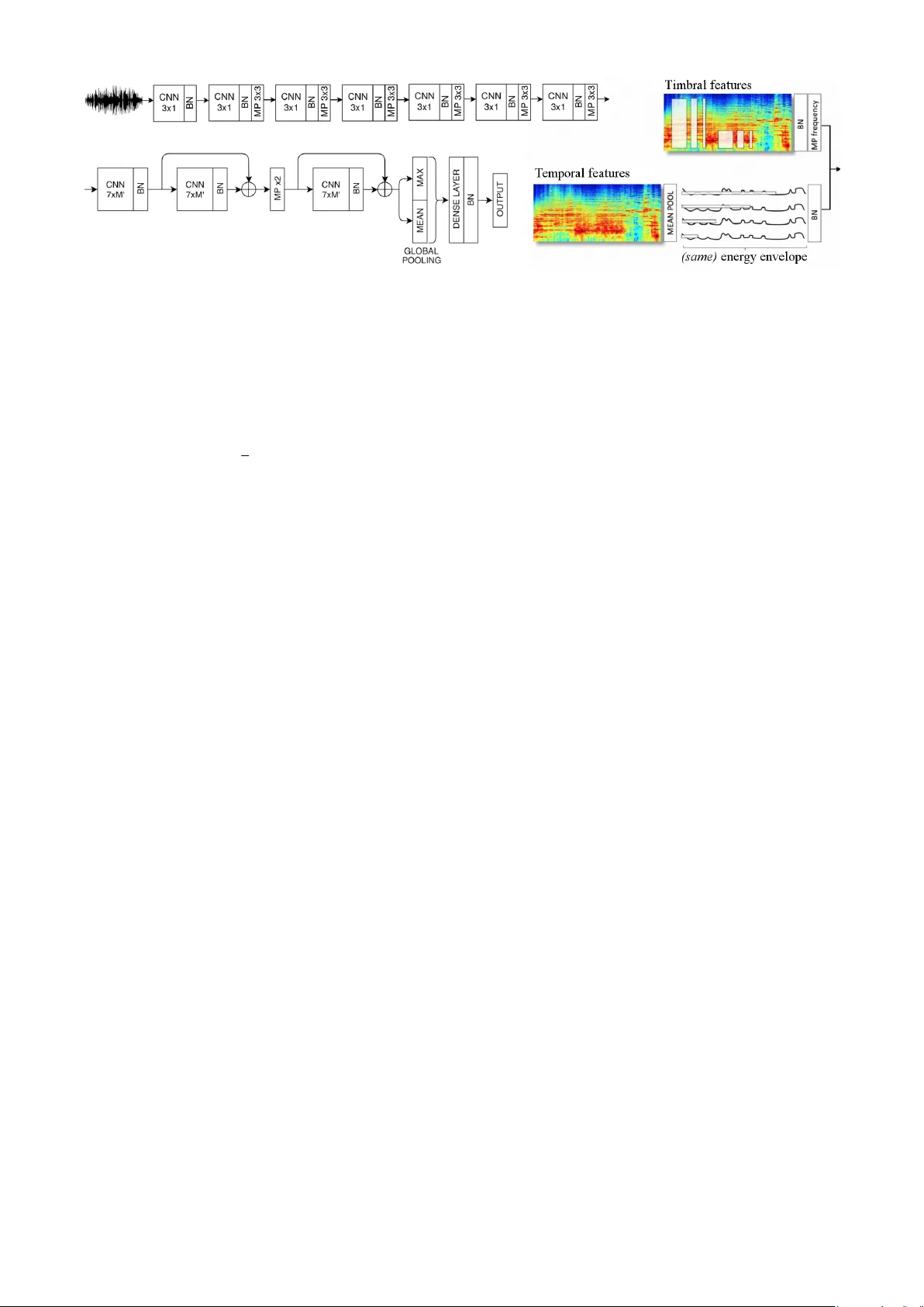
END-T O-END LEARNING FOR MUSIC A UDIO T A GGING A T SCALE Jordi Pons ? † Oriol Nieto † Matthew Prockup † Erik Schmidt † Andreas Ehmann † Xa vier Serra ? ? Music T echnology Group, Uni v ersitat Pompeu F abra, Barcelona † Pandora Media Inc., Oakland, CA ABSTRA CT The lack of data tends to limit the outcomes of deep learn- ing research, particularly when dealing with end-to-end learning stacks processing raw data such as wav eforms. In this study , 1.2M tracks annotated with musical la- bels are av ailable to train our end-to-end models. This large amount of data allows us to unrestrictedly explore two different design paradigms for music auto-tagging: assumption-free models – using wa veforms as input with very small con v olutional filters; and models that rely on domain knowledge – log-mel spectrograms with a con v o- lutional neural network designed to learn timbral and tem- poral features. Our work focuses on studying how these two types of deep architectures perform when datasets of variable size are av ailable for training: the MagnaT a- gA T une (25k songs), the Million Song Dataset (240k songs), and a priv ate dataset of 1.2M songs. Our experi- ments suggest that music domain assumptions are rele v ant when not enough training data are av ailable, thus show- ing ho w w av eform-based models outperform spectrogram- based ones in large-scale data scenarios. 1. INTR ODUCTION One fundamental goal in music informatics research is to automatically structure large music collections. The music audio tagging task consists of automatically estimating the musical attributes of a song – including: moods, language of the lyrics, year of composition, genres, instruments, har- mony , or rhythmic traits. Thus, tag estimates may be use- ful to define a semantic space that can be adv antageous for automatically organizing musical libraries. Many approaches ha v e been considered for this task (mostly based on feature extraction + model [1, 22, 26]), with recent publications showing promising results using deep architectures [5, 9, 14, 21]. In this work we confirm this trend by studying ho w two deep architectures con- ceiv ed considering opposite design strategies (using do- main knowledge or not) perform for several datasets – with one of the datasets being of an unprecedented size: 1.2M songs. Provided that a sizable amount of data is av ail- able for that study , we in v estigate the learning capabili- c  Jordi Pons, Oriol Nieto, Matthew Prockup, Erik Schmidt, Andreas Ehmann, Xavier Serra. Licensed under a Creativ e Commons Attribution 4.0 International License (CC BY 4.0). Attribu- tion: Jordi Pons, Oriol Nieto, Matthew Prockup, Erik Schmidt, Andreas Ehmann, Xavier Serra. “END-T O-END LEARNING FOR MUSIC A U- DIO T A GGING A T SCALE”, 19th International Society for Music Infor- mation Retriev al Conference, P aris, France, 2018. ties of these two architectures. Specifically , we in v esti- gate whether the architectures based on domain knowledge ov erly constrain the solution space for cases where large training data are av ailable – in essence, we study if certain architectural choices (e.g., using log-mel spectrograms as input) can limit the model’ s capabilities to learn from data. The main contribution of this work is to show that little to no model assumptions are required for music auto-tagging when operating with large amounts of data. Section 2 discusses the main deep architectures we identified in the audio literature, section 3 describes the datasets used for this work, section 4 presents the architec- tures we study , and section 5 pro vides discussion about the results with conclusions drawn in section 6. 2. CURRENT DEEP ARCHITECTURES In order to facilitate the discussion around the current au- dio architectures, we di vide deep learning models into tw o parts: front-end and back-end – see Figure 1. The front- end is the part of the model that interacts with the input signal in order to map it into a latent-space, and the back- end predicts the output given the representation obtained by the front-end. In the following, we present the main front- and back-ends we identified in the literature. Figure 1 . Deep learning pipeline. Front-ends. These are generally comprised of con- volutional neural networks (CNNs) [5, 9, 20, 21, 27], since these can learn efficient representations by sharing weights 1 along the signal. Front-ends can be divided into two groups depending on the used input signal: wave- forms [9, 14, 27] or spectrograms [5, 20, 21]. Further , the design of the filters can be either based on domain kno wl- edge or not. For example, one leverages domain knowl- edge when a front-end for wav eforms is designed so that the length of the filter is set to be as the window length of a STFT [9]. Or for a spectrogram front-end, it is used verti- cal filters to learn timbral representations [12] or horizontal filters to learn longer temporal cues [25]. Generally , a sin- gle filter shape is used in the first CNN layer [5, 9, 12, 25], but some recent works report performance gains when us- ing several filter shapes in the first layer [4, 18 – 21, 27]. Using many filters promotes a richer feature extraction in the first layer , and facilitates le veraging domain knowl- edge for designing the filters’ shape. For example: a 1 Which determine the learned feature representations. wa veform front-end using many long filters (of different lengths) can be motiv ated from the perspective of a multi- resolution time-frequency transform 2 [27]; or since it is known that some patterns in spectrograms are occurring at different time-frequency scales, one can intuitively in- corporate man y (dif ferent) vertical and/or horizontal filters in a spectrogram front-end [18 – 21]. T o summarize, using domain knowledge when designing models allo ws us to naturally connect the deep learning literature with previ- ous signal processing work. On the other hand, when do- main knowledge is not used, it is common to employ a deep stack of small filters, e.g.: 3 × 1 as in the sample-lev el front- end used for waveforms [14], or 3 × 3 filters used for spec- trograms [5]. These models based on small filters make minimal assumptions o ver the local stationarities of the signal, so that any structure can be learned via hierarchi- cally combining small-context representations. These ar - chitectures with small filters are flexible models able to po- tentially learn any structure gi v en enough depth and data. Back-ends. Among the different back-ends used in the audio literature, we identified two main groups: (i) fixed- length input back-end, and (ii) variable-length input back- end. The generally conv olutional nature of the front-end allows it to process different input lengths. Therefore, the back-end unit can adapt a v ariable-length feature map to a fix-sized output. The former group of models ( i ) assume that the input will be kept constant – examples of those are front-ends based on feed-forward neural-networks or fully-con v olutional stacks [5, 9]. The second group ( ii ) can deal with different input-lengths since the model is flexi- ble in at least one of its input dimensions – examples of those are back-ends using temporal-aggregation strategies such as max-pooling, a verage-pooling, attention models or recurrent neural networks [23]. Given that songs are gen- erally of different lengths, these types of back-ends are ideal candidates for music processing. Howe ver , despite the dif ferent-length nature of music, many works employ fixed-length input back-ends (group i ) since these architec- tures tend to be simpler and perform well [5, 9, 21]. 3. D A T ASETS W e study how different deep architectures for music auto- tagging perform for 3 music collections of different sizes: 1) The MagnaT agA Tune (MTT) dataset is o f ≈ 26k mu- sic audio clips of 30s [11]. Predicting the top-50 tags of this dataset is a popular benchmark for auto-tagging. 2) Although the Million Song Dataset (MSD) name in- dicates that 1M songs are av ailable [2], audio files with proper tag annotations (top-50 tags) are only av ailable for ≈ 240k previe ws of 30s. This dataset constitutes the biggest public dataset a v ailable for music auto-tagging, making these data highly appropriate for benchmarking. 3) A priv ate dataset consisting of 1M songs for training, 100k for validation, and 100k for test 3 is av ailable for this study . The 1.2M-songs dataset has 139 track-le v el human- expert annotations that can be summarized as follo ws: 2 The Constant-Q T ransform [3] is an example of such transform. 3 T est & v alidation sets are k ept the same throughout the e xperiments for a fair e valuation. All used partitions are stratified and artist-filtered. · Meter tags denote dif ferent sorts of musical meters (e.g., triple-meter , cut-time, compound-duple, odd). · Rhythmic feel tags denote rhythmic interpretation (e.g., swing, shuffle, back-beat strength) and elements of rhythmic perception ( e.g ., syncopation, danceability). · Harmonic tags : major , minor , chromatic, etc. · Mood tags express the sentiment of a music audio clip (e.g., if the music is angry , sad, joyful). · V ocal tags denote the presence of v ocals and timbral characteristics of it (e.g., male, female, vocal grittiness). · Instrumentation ta gs denote the presence of instru- ments (e.g., piano) and their timbre (e.g., guitar distortion). · Sonority tags detail production techniques (e.g., stu- dio, liv e) and o verall sound (e.g., acoustic, synthesized). · Basic genre tags : jazz, rock, rap, latin, disco, etc. · Subgenr e tags : jazz (e.g., cool, fusion, hard bop), rock (e.g., light, hard, punk), rap (e.g., east coast, old school), w orld music (e.g., cajun, indian), classical music (e.g., baroque period, classical period), etc. Other lar ge (music) audio datasets exist: the Free Music Archiv e (FMA: ≈ 106k songs) [8] and Audioset ( ≈ 2.1M audios) [10]. Since previous works mainly used the MTT and MSD [5, 14], we employ these datasets to assess the studied models with public data. Despite our interest in using FMA, for brevity , we restrict our study to 3 datasets that already cover a wide range of different sizes. Finally , Audioset is not used since most of its content is not music. 4. THE ARCHITECTURES UNDER STUD Y After an initial exploration of the dif ferent architectures in- troduced in section 2, we select two models based on op- posite design paradigms: one for processing wav eforms, with a design that does minimal assumptions over the task at hand; and another for spectrograms, with a design that heavily relies on musical domain kno wledge. Our goal is to compare these two models for providing insights in whether domain knowledge is required (or not) for design- ing deep learning models. This section provides discussion around our architectural choices and introduces the basic configuration setup – which is also accessible online. 4 The wav eform model was selected after observing that the sample-lev el front-end (using a deep stack of 3 × 1 fil- ters) was remarkably superior to the other wav eform-based front ends – as shown in the original paper [14]. This re- sult is particularly compelling because this front-end does not rely on domain-knowledge for its design. Note that raw wa v eforms are fed to the model without any pre- processing, and the small filters considered for its design make no strong assumptions ov er the most informative lo- cal stationarities in wa v eforms. Therefore, the sample- lev el can be seen as a problem agnostic front-end that has the potential to learn any audio task provided that enough depth and data are av ailable. Gi ven that a large amount data is av ailable for this study , the sample-le vel front-end is of particular interest due to its strong learning potential: its solution space is not constrained by sev ere architectural choices relying on domain knowledge. 4 https://github .com/jordipons/music-audio-tagging-at-scale-models Figure 2 . Bottom-left – back-end. T op-left – wav eform front-end. Right – spectrogram front-end. Definitions – M’ stands for the feature map’ s vertical axis, BN for batch norm, and MP for max-pool. On the other hand, when experimenting with spectro- gram front-ends, we found domain knowledge intuitions to be valid guides for designing deep architectures. For example, front-ends based on (i) many vertical and hori- zontal filters in the first layer were consistently superior to front-ends based on (ii) a single v ertical filter – as sho wn in recent publications [4, 18 – 20]. Note that the former front- ends (i) can learn spectral and (long) temporal represen- tations already in the first layer – which are known to be important musical cues; while the latter (ii) can only learn spectral representations. Moreo ver , we observed that front- ends based on a deep stack of 3 × 3 filters were achie ving equiv alent performances to the former front-end (i) when input segments were shorter than 10s – as noted in the lit- erature [21]. But when considering longer inputs (which yielded better performance), the computational price of this deeper model increases: longer inputs implies hav- ing larger feature maps in ev ery layer and therefore, more GPU memory consumption. F or that reason, we refrained from using a deep stack of 3 × 3 filters as a front-end – be- cause our 12GBs of VRAM were not enough to input 15s of audio when using a back-end. Hence, making use of domain knowledge also provides guidance for minimizing the computational cost of the model – since by using a sin- gle layer with many vertical and horizontal filters, one can efficiently capture the same recepti ve field without paying the cost of going deep. Finally , note that front-ends using many vertical and horizontal filters in the first layer are an example of deep architectures relying on (musical) domain knowledge for their design. After considering the previous discussion, we select the sample-lev el front-end as main part of our assumption-free model for w av eforms; and we use a spectrogram front-end with many vertical and horizontal (first-layer) filters for the model designed considering domain knowledge. Experi- ments below share the same back-end, which enables a fair comparison among the previously selected front-ends. Un- less otherwise stated, the following specifications are the ones used for the experiments – throughout the document, we refer to these specifications as the basic configuration: Shared back-end. It consists of three CNN layers (with 512 filters each and two residual connections), two pooling layers and a dense layer – see Figure 2 ( Bottom-left ). W e introduced residual connections in our model to e xplore very deep architectures, such that we can take advantage of the large data av ailable. Although adding more residual layers did not drastically impro ve our results, we observ ed that adding these residual connections stabilized learning while slightly improving performance [16]. The used 1D- CNN filters [9] are computationally efficient and shaped such that all e xtracted features are considered across a rea- sonable amount of temporal context (note the 7 × M’ filter shapes, representing time × all featur es ). W e also make a drastic use of temporal pooling: firstly , down-sampling x2 the temporal dimensionality of the feature maps; and sec- ondly , by making use of global pooling with mean and max statistics. The global pooling strategy allows for variable length inputs to the network and therefore, such a model can be classified as a “v ariable-length input” back-end. Fi- nally , a dense layer with 500 units connects the pooled fea- tures to a sigmoidal output. W av ef orm fr ont-end. It is based on a sample-lev el front-end [14] composed of seven: 1D-CNN (3 × 1 filters), batch norm, and max pool layers – see Figure 2 ( T op-left ). Each layer has 64, 64, 64, 128, 128, 128 and 256 filters. For the 1.2M-songs dataset, we use a model with more ca- pacity having nine layers with 64, 64, 64, 128, 128, 128, 128, 128, 256 filters. By hierarchically combining small- context representations and making use of max pooling, the sample-lev el front-end yields a feature map for an au- dio segment of 15s (do wn-sampled to 16kHz) which is fur - ther processed by the previously described back-end. Spectrogram front-end. Firstly , audio segments are con v erted to log-mel magnitude spectrograms (15 seconds and 96 mel bins [17]) and normalized to have zero-mean and unit-var . Secondly , we use vertical and horizontal fil- ters e xplicitly designed to facilitate learning the timbral and temporal patterns present in spectrograms [19–21]. Note in Figure 2 ( Right ) that the spectrogram front-end is a single-layer CNN with many filter shapes that are grouped into two branches [19]: (i ) top branch – tim- bral features [21]; and (ii) lower branch – temporal fea- tures [20]. The top branch is designed to capture pitch- in v ariant timbral features that are occurring at different time-frequency scales in the spectrogram. Pitch in variance is enforced via enabling CNN filters to con v olv e through the frequency domain, and via max-pooling the feature map across its v ertical axis [21]. Note that se veral fil- ter shapes are used to ef ficiently capture many different time-frequency patterns: 7 × 86, 3 × 86, 1 × 86, 7 × 38, 3 × 38 1.2M-songs train R OC PR Models size A UC A UC √ MSE Baseline 1.2M 91.61% 54.27% 0.1569 W aveform 1M 92.50 % 61.20 % 0.1465 Spectrogram 1M 92.17% 59.92% 0.1473 W aveform 500k 91.16% 56.42% 0.1504 Spectrogram 500k 91.61% 58.18% 0.1493 W aveform 100k 90.27% 52.76% 0.1554 Spectrogram 100k 90.14% 52.67% 0.1542 T able 1 . 1.2M-songs a verage results (3 runs) when using different training-set sizes. Baseline: GBTs+features [22]. and 1 × 38 5 – to facilitate learning, e.g.: kick-drums (with small-rectangular filters of 7 × 38 capturing sub-band in- formation for a short period of time), or string ensemble instruments (with long vertical filters of 1 × 86 which are capturing timbral patterns spread in the frequency axis). The lower branch is meant to learn temporal features, and is designed to ef ficiently capture different time-scale repre- sentations by using sev eral long filter shapes [20]: 165 × 1, 128 × 1, 64 × 1 and 32 × 1. 6 These filters operate over an en- ergy en v elope (not directly over the spectrogram) obtained via mean-pooling the frequency-axis of the spectrogram. By computing the ener gy en velope in that way , we are considering high and lo w frequencies together while min- imizing the computations of the model – note that no fre- quency/v ertical con volutions are performed, b ut 1D (tem- poral) conv olutions. Thus, domain knowledge is also pro- viding guidance to minimize the computational cost of the model. The output of these two branches is merged, and the previously described back-end is used for going deeper . For further details, see its online implementation. 4 Parameters. 50% dropout before e very dense layer, ReLUs as non-linearities, and our models are trained with SGD employing Adam (with an initial learning rate of 0.001) as optimizer . W e minimize the MSE for the 1.2M-songs dataset, but we minimize the cross entropy for the other datasets. During training our data are con verted to audio patches of 15s, but during prediction one aims to consider the whole song. T o this end, sev eral predictions are computed for a song (by a moving window of 15s) and then a veraged. Although our models are capable of pre- dicting tags for variable-length inputs, we use fixed length patches since in preliminary experiments we observed that predicting the whole song at once yielded worse results than av eraging several patch predictions. In future work we aim to further study this behavior , to find ways to ex- ploit the fact that the whole song is generally a v ailable. 5. EXPERIMENT AL RESUL TS 5.1 1.2M-songs dataset Experimental setup. As a baseline, we use a system consisting of a music feature extractor (in essence: tim- bre, rhythm, and harmony descriptors) and a model based on gradient boosted trees (GBT) for predicting each of the tags [22]. By predicting each tag individually , one aims 5 Each filter shape has 16, 32, 64, 16, 32 and 64 filters, respectiv ely . 6 Each filter shape has 16, 32, 64 and 128 filters, respectiv ely . Figure 3 . Linear regression fit on the 1.2M-songs results. to turn a hard problem into multiple (hopefully simpler ) problems. A careful inspection of the dataset reveals that, among tags, two dif ferent data distributions dominate the annotations: (i) tags with bi-modal distrib utions, where most of the annotations are zero, which can be classified; and (ii) tags with pseudo-uniform distributions that can be regressed. 7 A regression tag example is acoustic , which in- dicates how acoustic a song is – from zero to one, zero being an electronic music song and one a string quartet. And a classification tag example can be any genre – for example, most songs will not be cataloged as rap since the dataset is large and its taxonomy contains dozens of genres. W e use two sets of performance measurements: R OC-A UC 8 and PR-A UC 8 for the classification tags, and error ( √ M S E 8 ) for the regression tags. R OC-A UC can lead to over -optimistic scores in cases where data are un- balanced [7]; given that classification tags are highly un- balanced, we also consider the PR-A UC metric since it is more indicativ e than R OC-A UC in these cases [7]. For R OC-A UC and PR-A UC, the higher the score the better – but for √ M S E , the lower the better . Studied spectrogram and wav eform models are set follo wing the basic configu- ration – and are composed of 5.9M and 5.5M parameters, respectiv ely . Giv en the unprecedented size of the dataset, we focus on how these models scale when trained with dif- ferent amounts of data: 100k, 500k, or 1M songs. A verage results (across 3 runs) are shown in T able 1 and Figure 3. Quantitative results. T raining the models with 100k songs took a few days, with 500k songs one week, and with 1M songs less than two weeks. The deep learning models trained with 1M tracks achieve better results than the baseline in every metric. Howe v er , the deep learning models trained with 100k tracks perform worse than the baseline. This result confirms that deep learning models require large datasets to clearly outperform strong methods based on feature-design – although note that large datasets are generally not a v ailable for most audio tasks. Moreover , the biggest performance improv ement w .r .t. the baseline is seen for PR-A UC, which provides a more informati v e pic- ture of the performance when the dataset is unbalanced [7]. In addition, the best performing model is based on the wa veform front-end – being capable of outperforming the spectrogram model in ev ery metric when trained with 1M songs. This result confirms that w av eform sample-le vel front-ends ha ve a great potential to learn from large data, since their solution space is not constrained by any se- 7 Note that all output nodes are sigmoidal – i.e., we treat classification tags as regression tags for simplicity’ s sake. 8 R OC: Receiv er Operating Characteristic. PR: Precision Recall. A UC: Area Under the Curv e. MSE: Mean Squared Error. vere architectural choice. On the other hand, the architec- tural choices defining the spectrogram front-end might be constraining the solution space. While these architectural constraints are not harmful when training data are scarce (as for the 100k/500k songs results or in prior works [24]), such a strong regularization of the solution space may limit the learning capacity of the model in scenarios where large training data are av ailable – as for the 1M songs results. One can observe this in Figure 3, where we fit linear mod- els to the obtained results to further study this behavior . When 100k training songs are available: trend lines sho w that spectrogram models tend to perform better . Howe v er , when 1M training songs are av ailable: the lines show that wa veform models outperform the spectrogram ones. It is worth mentioning that the observed trends are consistent throughout metrics: ROC-A UC, PR-A UC, and √ M S E . Finally , note that there is room for impro ving the models under study – e.g.: one could address the data imbalance problem during training, or improve the back-end via ex- ploring alternativ e temporal aggre gation strategies. Qualitative results. Since it is the first report of a deep music tagging model trained with such a large dataset, we also perceptually assess the quality of the estimates. T o this end, we compared the predictions of one of our best per- forming models to the predictions of the baseline, and to the human-annotated ground-truth tags. Some interesting examples identified during this qualitativ e experiment are av ailable online. 9 First, we observed that the deep learning model is biased tow ards predicting the popular tags (such as lead vocals , English or male vocals ). Note that this is expected since we are not addressing the data unbalanc- ing issue during training. And second, we observe that the baseline model (which predicts the probability of each tag with an independent GBT model) predicts mutually exclu- siv e tags with high confidence – e.g., it predicted with high scores: East Coast and W est Coast for an East Cost rap song, or bar oque period and classic period for a Bach aria. Howe ver , the deep learning model (predicting the proba- bility of all tags together) was able to better differentiate these similar but mutually exclusi ve tags. This suggests that deep learning has an advantage when compared to tra- ditional approaches, since these mutually exclusi v e rela- tions can be jointly encoded within the model. 5.2 MagnaT agA T une (MTT) dataset Experimental setup. State-of-the-art models are set as baselines, and we use the same (classification) per- formance metrics as for the 1.2M-songs dataset: R OC- A UC and PR-A UC – note that the MTT labels are binary . One of the baseline results (the SampleCNN [14] with 90.55 R OC-A UC) was computed using a slightly different version of the MTT dataset – which only includes songs having more than 1 tag and lasting more than 29.1 sec- onds. As a result, this cleaner version of the MTT dataset is of ≈ 21k songs instead of ≈ 26k. Although this dataset cleans out potential noisy annotations, we decided to use the original dataset to easily compare our results with for- mer works. Thus, to fairly compare our models with 9 http://www .jordipons.me/apps/music-audio-tagging-at-scale-demo the SampleCNN, we reproduce their work considering the original dataset – achieving a score of 88.56 R OC-A UC. Giv en that less noise is present in the SampleCNN dataset, it seems reasonable that their performance is higher than the one obtained by our implementation. The MTT experiments can be divided in two parts: wa veform and spectrogram models – see T ables 2 and 3. Due to the amenable size of the dataset (ev ery MTT ex- periment lasts < 5h), it is feasible to run a comprehen- siv e study inv estigating different architectural configura- tions. Specifically , we study how wa v eform and spectro- gram architectures behav e when modifying the capacity of their front- and back-ends. For example, the experiment “# filters × 1/2” in T able 2 consists of dividing the num- ber of filters av ailable in the waveform front-end by two. This means ha ving 32, 32, 32, 64, 64, 64 and 128 filters, instead of the 64, 64, 64, 128, 128, 128 and 256 filters in the basic configuration. W e also apply this method- ology to the spectrogram front-ends, and we add/remove capacity to them by increasing/decreasing the number of av ailable filters. After running the front-end experiments with a fixed back-end (following the basic configuration: 512 CNN filters, 500 output units), we select the most promising ones to proceed with the back-end study – for wav eforms: “# filters × 2”, 10 and for spectrograms: “# filters × 1/2”. Having now a fixed front-end for e very experiment, we modify the capacity of the back-end via changing the number of filters in e very CNN layer (512, 256, 128, 64) and changing the number of output units (500, 200). Since the basic configuration leads to relatively big models for the size of the dataset, these experiments ex- plore smaller back-ends. The inputs for the MTT are set to be of 3s, since longer inputs yield worse results [15, 21]. Quantitative results. The wa veform and spectrogram models we study outperform the proposed baselines – which represent the current state-of-the-art. Further , per - formance is quite robust to the number of parameters of the model. Although the best results are achiev ed by mod- els having higher capacity , the performance difference be- tween small and lar ge models is minor – what means that relativ ely small models (which are easier to deploy) can do a reasonable job when tagging the MTT music. Finally: spectrogram models perform better than wav eform models for this small public dataset – which aligns with pre vious works using datasets of similar size [20, 21]. Consequently , these results confirm that domain knowledge intuitions are valid guides for designing deep architectures in scenarios where training data are scarce. 5.3 Million Song Dataset (MSD) Experimental setup. State-of-the-art models are set as baselines, and we use the same (classification) perfor- mance metrics as for the 1.2M-songs dataset: R OC-A UC and PR-A UC – note that the MSD labels are binary . These experiments aim to validate the studied models with the biggest public dataset av ailable. Models are set following the basic configuration, and results are sho wn in T able 4. 10 “# filters × 2” front-end was selected instead of “# filters × 4”, be- cause it performs similarly with less parameters. MTT dataset R OC PR # W aveform models A UC A UC param State-of-the-art r esults – with our own implementations SampleCNN [14] 13 90.55 - 2.4M SampleCNN (reproduced) 88.56 34.38 2.4M Dieleman et al. [9] 84.87 - - Dieleman et al. (reproduced) 85.58 29.59 194k How much capacity is r equir ed for the fr ont-end? # filters × 4 89.05 34.92 11.8M # filters × 2 (selected) 88.96 34.74 7M # filters × 1 88.9 34.18 5.3M # filters × 1/2 88.69 33.97 4.7M # filters × 1/4 88.47 33.89 4.4M How much capacity is r equir ed for the back-end? # filters in ev ery CNN layer - # units in dense layer 64 CNN filters - 500 units 88.57 33.99 1.3M - 200 units 88.94 34.47 1.3M 128 CNN filters - 500 units 88.82 34.62 1.8M - 200 units 88.81 34.6 1.7M 256 CNN filters - 500 units 88.95 34.27 3.1 M - 200 units 88.59 34.39 2.9M 512 CNN filters - 500 units 88.96 34.74 7M - 200 units 88.3 34.05 6.7M T able 2 . MTT results: wav eform models. Quantitative results. The spectrogram model outper- forms the wav eform model for this public dataset – hav- ing ≈ 200k training songs. Furthermore, the spectro- gram model performs equiv alently to ‘Multi-lev el & multi- scale’ [13], which is the best performing method in the lit- erature – denoting that musical kno wledge can be of utility to design models for the MSD. Additionally , the w av eform model performs worse than other wav eform-based mod- els that also employ sample-lev el front-ends. Such perfor- mance decrease could be caused because (i) SampleCNN methods [14, 15] a v erage ten 11 estimates for the same song to compensate for possible faults in song-lev el predictions, while our method only a verages two – predicting con- secutiv e patches of 15s; or (ii) because the major differ - ence between SampleCNN and the wa v eform model is that the latter employs a global pooling strategy that could re- mov e potentially useful information for the model. Be- sides, the best performing wa v eform-based model (‘Sam- pleCNN multi-lev el & multi-scale’ [15]) also achiev es lower scores than the best performing spectrogram-based ones. Considering the outstanding results we report when the wa v eform model is trained with 1M songs, one could argue that the lack of larger public datasets is limiting the outcomes of deep learning research for music auto- tagging – particularly when dealing with end-to-end learn- ing stacks processing raw data such as wa v eforms. 11 Since MSD audios are of 30s, ten tag estimates per song can be obtained via running the model with consecutiv e patches of 3s. 13 Result computed with a different MTT v ersion, see section 5.2. 14 Reproduced using 96 mel bands instead of 128 as in [21]. MTT dataset R OC PR # Spectr o gram models A UC A UC param State-of-the-art r esults – with our own implementations VGG - Choi et al. [5] 89.40 - 22M VGG (reproduced) 89.99 37.56 450k T imbre CNN [21] 89.30 - 191k T imbre CNN (reproduced) 14 89.07 34.92 220k How much capacity is r equir ed for the fr ont-end? # filters × 1/8 90.08 37.18 4.4M # filters × 1/4 90.12 37.69 4.6M # filters × 1/2 (selected) 90.40 38.11 5M # filters × 1 90.31 37.79 5.9 # filters × 2 90.07 37.29 7.6M How much capacity is r equir ed for the back-end? # filters in ev ery CNN layer - # units in dense layer 64 CNN filters - 500 units 90.03 36.98 277k - 200 units 90.28 37.55 222k 128 CNN filters - 500 units 90.16 37.61 617k - 200 units 90.28 37.69 524k 256 CNN filters - 500 units 90.18 37.98 1.6M - 200 units 90.06 37.16 1.4M 512 CNN filters - 500 units 90.40 38.11 5M - 200 units 89.98 37.05 4.7M T able 3 . MTT results: spectrogram models. 6. CONCLUSIONS This study presents the first work describing ho w dif ferent deep music auto-tagging architectures perform depending on the amount of a vailable training data. W e also present two architectures that yield results on par with the state- of-the-art. These architectures are based on two concep- tually different design principles: one is based on a wave- form front-end, and no domain knowledge inspired its de- sign; and the other , with a spectrogram front-end, makes use of (musical) domain knowledge to justify its architec- tural choices. While our results suggest that models rely- ing on domain knowledge play a relevant role in scenar- ios where no sizable datasets are av ailable, we have shown that, gi ven enough data, assumption-free models process- ing wa veforms outperform those that rely on musical do- main knowledge. MSD R OC PR # Models A UC A UC par am W aveform (ours) 87.41 28.53 5.3M SampleCNN [14] 88.12 - 2.4M SampleCNN multi-lev el 88.42 - - & multi-scale [15] Spectrogram (ours) 88.75 31.24 5.9M VGG + RNN [6] 86.2 - 3M Multi-lev el & 88.78 - - multi-scale [13] T able 4 . MSD results. T op – waveform-based models. Bottom – spectrogram-based models. 7. A CKNO WLEDGMENTS This work was partially supported by the Maria de Maeztu Units of Excellence Programme (MDM-2015-0502) – and we are grateful for the GPUs donated by NV idia. 8. REFERENCES [1] Y ann Bayle, Pierre Hanna, and Matthias Robine. Revisiting autotagging to ward faultless instrumental playlists generation. arXiv pr eprint arXiv:1706.07613 , 2017. [2] Thierry Bertin-Mahieux, Daniel PW Ellis, Brian Whit- man, and Paul Lamere. The million song dataset. In International Society for Music Information Retrieval Confer ence (ISMIR) , 2011. [3] Judith C Brown. Calculation of a constant q spectral transform. The J ournal of the Acoustical Society of America , 89(1):425–434, 1991. [4] Ning Chen and Shijun W ang. High-lev el music de- scriptor extraction algorithm based on combination of multi-channel cnns and lstm. In International Society for Music Information Retrieval Confer ence (ISMIR) , 2017. [5] Keunwoo Choi, Geor ge Fazekas, and Mark Sandler . Automatic tagging using deep conv olutional neural networks. International Society for Music Information Retrieval Confer ence (ISMIR) , 2016. [6] Keunwoo Choi, Gy ¨ orgy Fazekas, Mark Sandler, and Kyungh yun Cho. Conv olutional recurrent neural net- works for music classification. In IEEE International Confer ence on Acoustics, Speech and Signal Pr ocess- ing (ICASSP) , 2017. [7] Jesse Davis and Mark Goadrich. The relationship between precision-recall and roc curves. In Inter- national Conference on Machine Learning (ICML) . A CM, 2006. [8] Micha ¨ el Defferrard, Kirell Benzi, Pierre V an- derghe ynst, and Xavier Bresson. Fma: A dataset for music analysis. In International Society for Music Information Retrieval Confer ence (ISMIR) , 2017. [9] Sander Dieleman and Benjamin Schrauwen. End-to- end learning for music audio. In IEEE International Confer ence on Acoustics, Speech and Signal Pr ocess- ing (ICASSP) , 2014. [10] Jort F Gemmeke, Daniel PW Ellis, Dylan Freedman, Aren Jansen, W ade Lawrence, R Channing Moore, Manoj Plakal, and Marvin Ritter . Audio set: An on- tology and human-labeled dataset for audio e vents. In IEEE International Confer ence on Acoustics, Speech and Signal Processing (ICASSP) , 2017. [11] Edith Law , Kris W est, Michael I Mandel, Mert Bay , and J Stephen Downie. Evaluation of algorithms using games: The case of music tagging. In International So- ciety for Music Information Retrieval Conference (IS- MIR) , 2009. [12] Honglak Lee, Peter Pham, Y an Largman, and An- drew Y Ng. Unsupervised feature learning for au- dio classification using con v olutional deep belief net- works. In Advances in Neural Information Pr ocessing Systems , 2009. [13] Jongpil Lee and Juhan Nam. Multi-lev el and multi- scale feature aggregation using pretrained con volu- tional neural networks for music auto-tagging. IEEE signal pr ocessing letters , 24(8):1208–1212, 2017. [14] Jongpil Lee, Jiyoung Park, Keunhyoung Luk e Kim, and Juhan Nam. Sample-lev el deep con v olutional neural networks for music auto-tagging using raw wa veforms. Sound and Music Computing Confer ence (SMC) , 2017. [15] Jongpil Lee, Jiyoung Park, Keunhyoung Luk e Kim, and Juhan Nam. Samplecnn: End-to-end deep con v olu- tional neural networks using very small filters for mu- sic classification. Applied Sciences , 8(1):150, 2018. [16] Hao Li, Zheng Xu, Gavin T aylor, and T om Goldstein. V isualizing the loss landscape of neural nets. arXiv pr eprint arXiv:1712.09913 , 2017. [17] Geoffroy Peeters. A large set of audio features for sound description (similarity and classification) in the cuidado project. 2004. [18] Huy Phan, Lars Hertel, Marco Maass, and Alfred Mertins. Rob ust audio event recognition with 1-max pooling con volutional neural networks. arXiv pr eprint arXiv:1604.06338 , 2016. [19] Jordi Pons, Thomas Lidy , and Xavier Serra. Experi- menting with musically motiv ated conv olutional neural networks. In 14th International W orkshop on Content- Based Multimedia Indexing (CBMI) , pages 1–6. IEEE, 2016. [20] Jordi Pons and Xa vier Serra. Designing ef ficient archi- tectures for modeling temporal features with con vo- lutional neural networks. In IEEE International Con- fer ence on Acoustics, Speech and Signal Pr ocessing (ICASSP) , 2017. [21] Jordi Pons, Olga Slizovskaia, Rong Gong, Emilia G ´ omez, and Xavier Serra. Timbre analysis of music au- dio signals with con v olutional neural networks. Eur o- pean Signal Pr ocessing Conference (EUSIPCO2017) , 2017. [22] Matthew Prockup, Andrew J. Asman, Fabian Gouyon, Erik M. Schmidt, Oscar Celma, and Y oungmoo E. Kim. Modeling rhythm using tree ensembles and the music genome project. Machine Learning for Music Discovery W orkshop at the International Conference on Machine Learning (ICML) , 2015. [23] Colin Raffel. Learning-Based Methods for Comparing Sequences, with Applications to Audio-to-MIDI Align- ment and Matching . PhD thesis, 2016. [24] T ara N Sainath, Ron J W eiss, Andrew Senior , K e vin W W ilson, and Oriol V in yals. Learning the speech front- end with raw waveform cldnns. In Sixteenth Annual Confer ence of the International Speech Communica- tion Association , 2015. [25] Jan Schluter and Sebastian Bock. Improv ed musical onset detection with con volutional neural networks. In IEEE International Confer ence on Acoustics, Speech and Signal Processing (ICASSP) , 2014. [26] Mohamed Sordo, Cyril Laurier , and Oscar Celma. An- notating music collections: How content-based simi- larity helps to propagate labels. In International So- ciety for Music Information Retrieval Conference (IS- MIR) , 2007. [27] Zhenyao Zhu, Jesse H Engel, and A wni Hannun. Learning multiscale features directly from wav eforms. arXiv pr eprint arXiv:1603.09509 , 2016.