Split-door criterion: Identification of causal effects through auxiliary outcomes

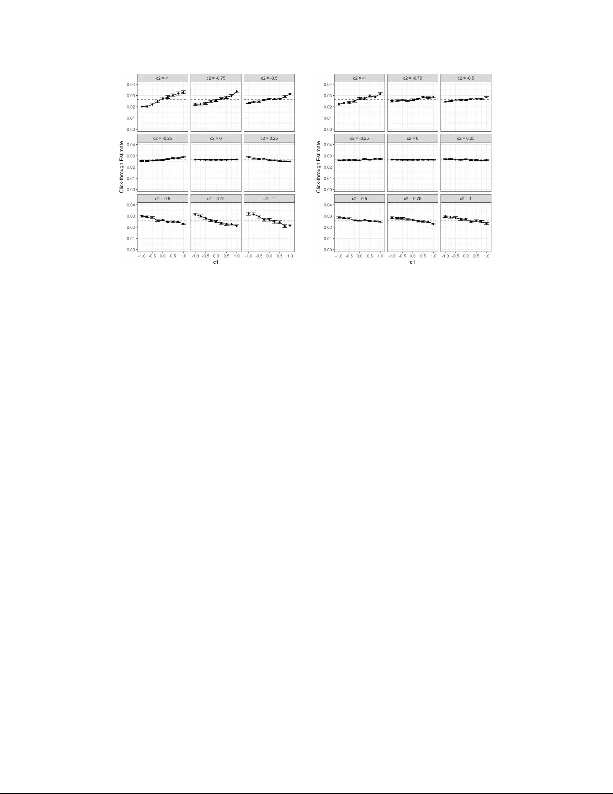
arXiv: SPLIT-DOOR CRITERION: IDENTIFICA TION OF CA USAL EFFECTS THR OUGH A UXILIAR Y OUTCOMES By Amit Sharma , Jake M. Hofman and Duncan J. W a tts Micr osoft R ese ar ch W e present a metho d for estimating causal eﬀects in time series data when ﬁne-grained information ab out the outcome of in terest is av ailable. Speciﬁcally , w e examine what w e call the split-door setting, where the out- come v ariable can b e split into t wo parts: one that is p oten tially aﬀected by the cause being studied and another that is indep enden t of it, with both parts sharing the same (unobserved) confounders. W e show that un- der these conditions, the problem of iden tiﬁcation reduces to that of testing for independence among observ ed v ariables, and presen t a method that uses this approach to automatically ﬁnd subsets of the data that are causally identiﬁed. W e demonstrate the method b y estimating the causal impact of Amazon’s recommender system on traﬃc to product pages, ﬁnding thou- sands of examples within the dataset that satisfy the split-door criterion. Unlike past studies based on natural exp erimen ts that were limited to a single product category , our metho d applies to a large and representative sample of products viewed on the site. In line with previous work, we ﬁnd that the widely-used click-through rate (CTR) metric o verestimates the causal impact of recommender systems; depending on the product category , we estimate that 50-80% of the traﬃc attributed to recommender systems would hav e happened ev en without any recommendations. W e conclude with guidelines for using the split-do or criterion as w ell as a discussion of other con texts where the metho d can be applied. 1. In tro duction. The recent gro wth of digital platforms has generated an av alanc he of highly gran ular and often longitudinal data regarding individual and collectiv e b eha v- ior in a v ariet y of domains of in terest to researc hers, including in e-commerce, health- care, and so cial media consumption. Because the v ast ma jority of this data is generated in non-exp erimen tal settings, researc hers typically m ust deal with the p ossibilit y that an y causal eﬀects of in terest are complicated b y a num b er of potential confounds. F or example, even eﬀects as conceptually simple as the causal impact of recommendations on customer purc hases are lik ely confounded b y selection eﬀects [ Lewis, Rao and Reiley , 2011 ], correlated demand [ Sharma, Hofman and W atts , 2015 ], or other shared causes of b oth exp osure and purc hase. Figure 1a sho ws this canonical class of causal inference problems in the form of a causal graphical mo del [ Pearl , 2009 ], where X is the cause and Y is its eﬀect. T ogether U and W refer to all of the common causes of X and Y that ma y confound estimation of the causal eﬀect, where critically some of these confounders (lab eled W ) may be observ ed, while others ( U ) are unobserved or even unkno wn. Ideally one w ould answer suc h questions b y running randomized experiments on these platforms, but in practice such tests are p ossible only for the o wners of the platform in question, and ev en then are often b eset with implemen tation diﬃculties or ethical concerns [ Fiske and Hauser , 2014 ]. As a result researchers are left with tw o main strategies for making causal estimates from large-scale observ ational data, eac h with its own assumptions and limitations: either conditioning on observ ables or exploiting natural experiments. 1.1. Backgr ound: Back-do or criterion and natur al exp eriments. The ﬁrst and by far the more common approach is to assume that the eﬀect of unobserved confounders ( U ) is negligible after conditioning on the observ ed v ariables ( W ). Under such a sele ction on observables assumption [ Im b ens and Rubin , 2015 ], one conditions on W to estimate the ∗ W e would like to thank Dean Ec kles, Praneeth Netrapalli, Joshua Angrist, T. T ony Ke, and anony- mous review ers for their valuable feedback on this work. Keywor ds and phr ases: causal inference, data mining, causal graphical mo del, natural exp erimen t, recommendation systems 1 2 SHARMA ET AL. W Y X U (a) Canonical causal in- ference problem W Y X (b) Estimation with b ack-do or criterion U Y X Z (c) Estimation with Z as an instrumental variable Fig 1: L eft: Graphical model for the canonical problem in causal inference. W e wish to estimate the eﬀect of X on Y . W represents observ ed common causes of X and Y ; U represen ts other unobserved (and unkno wn) common causes that confound observ ational estimates. Midd le : The causal mo del under the sele ction on observables assumption, where there are no kno wn unobserved confounds U . Right: The canonical causal mo del for an instrumental v ariable Z that systematically shifts the distribution of the cause X indep enden tly of confounds U . eﬀect of X on Y when these confounders are held constant. In the language of graph- ical models, this strategy is referred to as the b ack-do or criterion [ P earl , 2009 ] on the grounds that the “back-door pathw ay” from X to Y (via W) is block ed by condition- ing on W (see Figure 1b ) and can be implemen ted b y a v ariety of methods, including regression, stratiﬁcation, and matching [ Rubin , 2006 ; Stuart , 2010 ]. Unfortunately for most practical problems it is diﬃcult to establish that all of the important confounders ha ve been observed. F or example, consider the problem of estimating the causal impact of a recommender sys tem on traﬃc to e-commerce websites such as Amazon.com, where X corresp onds to the num b er of visits to a product’s webpage, and Y the visits to a recommended product shown on that w ebpage. One could compute the observed click- through rate after conditioning on all av ailable user and product attributes (e.g., user demographics, product categories and p opularities, etc.), assuming that these features constitute a pro xy for latent demand. Unfortunately , there are also many p oten tially unobserv ed confounders (e.g., advertising, media co verage, seasonality , etc.) that impact b oth a pro duct and its recommendations, which if excluded would render the bac k-do or criterion in v alid. Motiv ated b y the limitations of the back-door strategy , a second main approac h is to iden tify an external ev ent that aﬀects the treatmen t X in a w ay that is arguably ran- dom with resp ect to p oten tial confounds. The hope is that suc h v ariation, kno wn as a natur al exp eriment [ Dunning , 2012 ], can serv e as a substitute for an actual randomized exp erimen t. Con tinuing with the problem of estimating the causal impact of recommen- dations, one migh t lo ok for a natural exp erimen t in whic h some pro ducts exp erience large and sudden changes in traﬃc, for instance when a b ook is featured on Oprah’s b ook club [ Carmi, Oestreicher-Singer and Sundarara jan , 2012 ]. Assuming that the in- crease in traﬃc for the bo ok is independent of demand for its recommendations, one can estimate the causal eﬀect of the recommender by measuring the change in sales to the recommended products b efore and after the bo ok w as featured, arguing that these sales w ould not ha ve happ ened in the absence of the recommender. Suc h ev ents pro vide in- strumental variables that identify the eﬀect of interest by shifting the distribution of the cause X indep enden tly of unobserved confounds U [ Angrist, Imbens and Rubin , 1996 ]. Figure 1c depicts this in a graphical mo del, where the additional observed v ariable Z denotes the instrumen tal v ariable. These tw o main approaches trade oﬀ critical goals of iden tiﬁcation and generalization in causal inference. The estimate for back-door conditioning is t ypically derived using all a v ailable data, but pro vides no identiﬁcation guarantees in the presence of unobserv ed SPLIT-DOOR CRITERION F OR CA USAL IDENTIFICA TION 3 U X X U Y Y R Y D (a) General split-door mo del: Outcome Y is split in to Y R and Y D U X X U Y Y R Y D (b) V alid split-door mo del: Data subsets where X is independent of U Y Fig 2: P anel (a) illustrates the canonical causal inference problem when outcome Y can b e split up into t wo components. F or clarit y , unobserv ed confounders U are broken in to U Y that aﬀects b oth X and Y , and U X that aﬀects only X . The split-door criterion ﬁnds subsets of the data where the cause X is independent of U Y b y testing indep endence of X and Y D , leading to the unconfounded causal mo del sho wn in Panel (b). confounders. Instrumental v ariables, in contrast, pro vide iden tiﬁcation guarantees even in the presence of unobserv ed confounders, but these guarantees apply only for lo cal subsets of the a v ailable data—the relatively rare instances for whic h a v alid instrument that exogenously v aries the cause X is kno wn (e.g., lotteries [ Angrist, Im b ens and Rubin , 1996 ], v ariation in weather [ Phan and Airoldi , 2015 ], or sudden, large even ts [ Rosenzweig and W olpin , 2000 ; Dunning , 2012 ]). 1.2. The “split-do or” criterion. In this pap er we introduce a causal identiﬁcation strategy that incorporates elemen ts of both the back-door and natural exp erimen t ap- proac hes, but that applies in a diﬀeren t setting. Rather than conditioning on observ able confounds W or exploiting sources of indep enden t v ariation in the cause X , we instead lo ok to auxiliary outc omes [ Mealli and Pacini , 2013 ] to iden tify subsets of the data that are causally iden tiﬁed. Speciﬁcally , our strategy applies when the outcome v ariable Y can b e eﬀectively “split” in to tw o constituen ts: one that is caused b y X and another that is indep enden t of it. Figure 2a shows the corresponding causal graphical mo del, where Y R denotes the “referred” outcome of interest aﬀected b y X and Y D indicates the “direct” constituen t of Y that do es not directly dep end on X . Returning to the recommender sys- tem example, Y R corresp onds to recommendation clic k-throughs on a pro duct whereas Y D w ould b e all other traﬃc to that pro duct that comes through channels such as direct searc h or browsing. Whenev er such ﬁne-grained data on Y is av ailable, we sho w that it is p ossible to reduce causal iden tiﬁcation to an indep endence test b et ween the cause X and the auxiliary outcome Y D . Because this strategy depends on the a v ailability of a split set of v ariables for Y , w e call it the split-do or criterion for causal identiﬁcation, by analogy with the more familiar bac k-do or criterion. Although we mak e no assumptions ab out the functional form of relationships b et w een v ariables, a crucial assumption underlying the split-do or criterion is c onne cte dness ; i.e., that the auxiliary outcome Y D m ust b e aﬀected (possibly diﬀerently) b y al l causes that also aﬀect Y R . As w e discuss in more detail in Section 5 , this assumption is plausible in scenarios suc h as online recommender systems, where recommended pro ducts are reach- able through multiple c hannels (e.g., searc h or direct navigation) and it is unlikely that demand for a pro duct manifests itself exclusiv ely through only one of these channels. More generally , the connectedness assumption is exp ected to hold in scenarios where direct and referred outcomes incur similar cost, which mak es it unlikely that something that causes the outcome does so only when referred through X , but nev er directly . Under the ab o v e assumption, the split-do or criterion seeks to identify subsets of the data where causal iden tiﬁcation is possible. In this sense, the metho d resem bles a natural 4 SHARMA ET AL. exp erimen t, except that instead of lo oking for an instrument that creates v ariation in X , w e lo ok for v ariations in X directly . As in a natural exp erimen t, ho wev er, it is important that any suc h v ariation in X is indep enden t of p oten tial confounds. F or instance in the example abov e, it is imp ortan t that a sudden burst of interest in a particular b ook is not correlated with changes in laten t demand for its recommendations. T o v erify this requiremen t, the split-do or criterion relies on a s tatistical test to select for cases where there are no confounds (observed or otherwise) b et ween X and Y R . Sp eciﬁcally , w e show that given a suitable auxiliary outcome Y D , and a test to establish if X and Y D are indep enden t, the causal eﬀect b et w een X and Y R can be identiﬁed. F urthermore, since this test inv olves tw o observed quan tities ( X and Y D ), we can systematically search for subsets of the data that satisfy the required condition, p oten tially discov ering a large n umber of cases in whic h we can identify the causal eﬀect of X on Y R . W e illustrate this metho d with a detailed example in which we estimate the causal impact of Amazon.com’s recommendation system using historical web browsing data. Under the ab o ve assumptions on the dependence betw een referred and direct visits to a pro duct’s webpage, w e show ho w the criterion provides a principled mechanism for determining which subsets of the data to include in the analysis. The split-door criterion iden tiﬁes thousands of suc h instances in a nine-mon th p eriod, comparable in magnitude to a man ually tuned approach using the same data [ Sharma, Hofman and W atts , 2015 ], and an order of magnitude more than traditional approac hes [ Carmi, Oestreicher-Singer and Sundarara jan , 2012 ]. F urther, the pro ducts included in our analysis are represen ta- tiv e of the o verall pro duct distribution o ver pro duct categories on Amazon.com, thereb y impro ving both the precision and generalizabilit y of estimates. Consistent with previous w ork [ Sharma, Hofman and W atts , 2015 ], we ﬁnd that observ ational estimates of rec- ommendation clic k-through rates (CTRs) o verstate the actual eﬀect by anywhere from 50% to 80%, calling into question the v alidit y of p opular CTR metrics for assessing the impact of recommendation systems. F or applications to other online and oﬄine scenarios, w e pro vide an R pac k age 1 that implemen ts the split-door criterion. 1.3. Outline of p ap er. The remainder of this pap er proceeds as follo ws. In Section 2 w e start with a formal deﬁnition of the split-door criterion and giv e precise conditions un- der which the criterion holds. F or clarity we provide pro ofs for causal identiﬁcation b oth in terms of the causal graphical mo del from Figure 2a and also in terms of structural equations. In Section 3 we prop ose a simple, scalable algorithm for identifying causal eﬀects using the split-do or criterion. Then in Section 4 , w e explain more formally ho w the split-door criterion diﬀers from the instrumental v ariables and bac k-do or methods men tioned abov e. Section 5 presents details ab out the Amazon.com data and an appli- cation of the split-do or criterion to estimate the causal impact of its recommendation system. In Section 6 we then discuss limitations of the split-do or criterion as w ell as other settings in whic h the criterion applies, arguing that man y existing datasets across a v ariet y of domains ha v e the structure that outcomes of in terest can be decomp osed in to their “direct” and “referred” constituents. W e conclude with a prediction that as the size and gran ularit y of a v ailable datasets, along with the n umber of v ariables in them, in- crease at an ever faster rate, data-driven approaches to causal identiﬁcation will become commonplace. 2. The Split-door Iden tiﬁcation Criterion. The split-door criterion can be used whenev er observ ed data is generated from the model sho wn in Figure 2a . Here X repre- sen ts the cause of interest, Y R denotes the “referred” portion of the outcome aﬀected by it, and Y D indicates the “direct” part of the outcome whic h does not directly depend on X . W e denote the ov erall outcome b y Y = Y R + Y D . W e let U Y represen t all unobserved causes of Y , some of which ma y also b e common causes of X , hence the arrow from U Y to X . Additional late n t factors that aﬀect only X are captured b y U X . Both U X and U Y 1 URL: http://www.github.com/amit- sharma/splitdoor- causal- criterion SPLIT-DOOR CRITERION F OR CA USAL IDENTIFICA TION 5 can b e a combination of man y v ariables, some observed and some unobserved. (F or full generalit y , the analysis presented here assumes that all confounds are unobserv ed.) A s noted earlier, the unobserved v ariables U Y create “bac k-do or path wa ys” that confound the causal eﬀect of X on Y , resulting in biased estimates. The central idea b ehind the split-do or criterion is that we can use an independence test b et ween the auxiliary out- come Y D and X to systematically searc h for subsets of the data that are free of these confounds and do not con tain bac k-do or pathw ays b et ween X and Y R . In other words, w e can conclude that such subsets of the data were generated from the unconfounded causal model shown in Figure 2b , and therefore the causal eﬀect of X on Y can be esti- mated directly from these data. Imp ortan tly , identiﬁcation of the causal eﬀect rests on the assumption that no part of U Y causes one part of Y and not the other. 2.1. The split-do or criterion thr ough a gr aphic al mo del. Here w e formalize the in tu- ition abov e in the causal graphical mo del framework. T o iden tify the causal eﬀect, we mak e the follo wing tw o assumptions. The ﬁrst pertains to connectedness of the causal mo del. Assumption 1 (Connectedness) . Any unobserve d c onfounder U Y that c auses b oth X and Y R also c auses Y D and the c ausal eﬀe ct of such U Y on Y D is non-zer o. Note that Assumption 1 requires only that the causal eﬀect of U Y on Y D b e non- zero, without any requiremen ts on the size of the eﬀect(s) in volv ed. That said, it is a strong requiremen t in general, as it applies to all sub-comp onen ts of U Y and th us in v olv es assumptions ab out potentially high-dimensional, unobserv ed v ariables. Whenever Y D and Y R are comp onen ts of the same v ariable it is plausible that they share causes, but one still m ust establish that this condition holds to ensure causal iden tiﬁcation. It is instructive to compare this assumption to the strict independence assumptions in volving unobserv ed confounders required by metho ds suc h as instrumen tal v ariables [ Angrist, Im b ens and Rubin , 1996 ]. The second assumption, which relates statistical and causal indep endence b et ween observ ed v ariables, is standard for many metho ds of causal disco very from observ ational data. Assumption 2 (Indep endence) . If X and Y D ar e statistic al ly indep endent, then they ar e also c ausal ly indep endent in the gr aphic al mo del of Figur e 2a . Here c ausal independence betw een tw o v ariables means that they share no common causes and no directed path in the causal graphical mo del leads from one to another. More formally , the tw o v ariables are “d-sep ar ate d” [ Pearl , 2009 ] from each other. Thus, Assumption 2 is a v ariant of the F aithfulness or Stability assumptions in causal graphs with laten t unobserved v ariables [ Spirtes, Glymour and Scheines , 2000 ; Pearl , 2009 ]. In the causal mo del shown in Figure 2a , for instance, this assumption rules out the p ossibilit y of an ev ent where the observed v ariables X and Y D are found to b e statistically indep enden t, but U Y still aﬀects b ot h of them and the observ ed indep endence in the data results from U Y ’s eﬀect canceling out exactly o ver the path X - U Y - Y D . In other w ords, this assumption serves to rule out an (unlik ely) even t where incidental equalit y of parameters or certain data distributions render t wo v ariables statistically indep enden t even though they are causally related. Under Assumptions 1 and 2, we can sho w that statistical indep endence of X and Y D ensures that X is not confounded b y U Y . First, w e pro vide a result ab out the resulting causal graph structure when X ⊥ ⊥ Y D . Lemma 1 . L et X , Y R and Y D b e thr e e observe d variables c orr esp onding to the c ausal mo del in Figur e 2a , wher e U Y r efers to unobserve d c auses of Y R . If the c onne cte dness (1) and indep endenc e (2) assumptions hold, then X ⊥ ⊥ Y D implies that the e dge U Y → X do es not exist or that U Y is c onstant. 6 SHARMA ET AL. Pr o of (A r gument). The pro of can b e completed directly from Figure 2a and prop erties of a causal graphical model. X ⊥ ⊥ Y D implies that the causal eﬀect of U Y on Y D and X somehow cancels out on the path X ← U Y → Y D . By Assumption 2 , this cancellation is not due to inciden tal equalit y of parameters or a particular data distribution, but rather a prop ert y of the causal graphical model. Therefore, this can only happen if (i) U Y is constan t (and th us blo cks the path), or (ii) One of the edges exists trivially (do es not ha ve a causal eﬀect). Using Assumption 1 , U Y has a non-zero eﬀect on Y D . Then, the only alternative is that the X ← U Y edge do es not exist, leading to the unconfounded causal model in Figure 2b . Proof. W e pro vide a pro of by con tradiction using the principle of d-sep ar ation [ Pearl , 2009 ] in a causal graphical mo del. Let us suppose X ⊥ ⊥ Y D , and that the U Y → X edge exists and U Y is not constan t. Using the rules of d-sep ar ation on the causal mo del in Figure 2a , the path X - U Y - Y D corresp onds to: ( X ⊥ ⊥ Y D | U Y ) G (2.1) ( X 6 ⊥ ⊥ Y D ) G (2.2) where the notation ( . ) G refers to d-sep ar ation under a causal mo del G . In our case, G corresp onds to the causal mo del in Figure 2a . Ho wev er, using Assumption 2, statistical indep endence of X and Y D implies causal indep endence, and thus, d-separation of X and Y D . ( X ⊥ ⊥ Y D ) G (2.3) Equations 2.2 and 2.3 result in a contradiction. T o resolv e, (i) Either U Y is constan t and th us 2.1 implies ( X ⊥ ⊥ Y D ) G holds, or (ii) The path X - U Y - Y D do es not exist. Using Assumption 1 of dependence of Y D on U Y , the only possibility is that the X ← U Y edge does not exist. W e no w sho w that Lemma 1 remov es confounding due to U Y and that the observ ational estimate P ( Y R | X = x ) is also the causal estimate. Theorem 2.1 (Split-do or Criterion) . Under the assumptions of L emma 1 , the c ausal eﬀe ct of X on Y R is not c onfounde d by U Y and is given by: P ( Y R | do ( X = x )) = P ( Y R | X = x ) wher e do ( X = x ) r efers to exp erimental manipulation of X and Y R | X = x r efers to the observe d c onditional distribution. Pr o of (A r gument). Lemma 1 leads to tw o cases: (i) By the bac k-do or criterion [ Pearl , 2009 ], if U Y is constant, then X and Y R are uncon- founded, because the only back-door path betw een X and Y R con tains U Y on it. (ii) Similarly , if the U Y → X edge do es not exist, then X and Y R are unconfounded b ecause absence of the U Y → X edge remov es the back-door path b et ween X and Y R . In both cases, unconfoundedness implies that the eﬀect of X on Y R can be estimated using the observ ational distribution. Proof. The pro of follo ws from an application of the second rule of do-calculus [ P earl , 2009 ]. P ( Y | do ( Z = z ) , W ) = P ( Y |Z = z , W ) if ( Y ⊥ ⊥ Z |W ) G Z (2.4) SPLIT-DOOR CRITERION F OR CA USAL IDENTIFICA TION 7 where G Z refers to the underlying causal graphical mo del with all outgoing edges from Z remo ved. Substituting Y = Y R , Z = X , G X corresp onds to the causal model from Figure 2a without the X → Y R edge. Using Lemma 1 , t wo cases exist: (i) U Y is constan t Let W = U Y . Under the modiﬁed causal mo del G X without the X → Y R edge, the path X - U Y - Y R is the only path connecting X and Y R , whic h leads to the follo wing d-sep ar ation result: ( Y R ⊥ ⊥ X | U Y ) G X (2.5) Com bining Rule 2.4 and the abov e d-sep ar ation result, w e obtain P ( Y R | do ( X = x ) , U Y ) = P ( Y R | X = x, U Y ) = P ( Y R | X = x ) where the last equalit y holds b ecause U Y is constan t throughout. (ii) The edge U Y → X do es not exist. Let W = ∅ . Under the modiﬁed causal model G X without the X → Y R edge, X and Y R are trivially d-sep ar ate d b ecause no path connects them without the edge U Y → X . ( Y R ⊥ ⊥ X ) G X (2.6) F rom Rule 2.4 and the abov e d-sep ar ation result, w e obtain P ( Y R | do ( X = x )) = P ( Y R | X = x ) 2.2. The split-do or criterion thr ough structur al e quations. Although we hav e already analyzed the split-do or criterion in terms of the causal graphical mo del in Figure 2a , for exp ositional clarit y we note that it is also possible to do the same using structural equations. Speciﬁcally , w e can write three structural equations: x = g ( u x , u y , ε x ) y r = f ( x, u y , ε y r ) y d = h ( u y , ε y d ) , (2.7) where ε x , ε y r , and ε y d are m utually indep enden t, zero-mean random v ariables that cap- ture mo deling error and statistical v ariability . As in Assumption 1 , w e assume that U Y aﬀects b oth Y D and Y R . In general, the causal eﬀects among v ariables may not b e linear; ho wev er, for the purpose of building intuition w e rewrite the ab o v e equations in linear parametric form: x = ηu x + γ 1 u y +  x y r = ρx + γ 2 u y +  y r y d = γ 3 u y +  y d , (2.8) where ρ is the causal parameter of interest, and  x ,  y r  y d are indep enden t errors in the regression equations. The split-do or criterion requires indep endence of X and Y D , which in turn implies that Co v( X , Y D ) = 0: 0 = Co v( X , Y D ) = E[ X Y D ] − E[ X ] E[ Y D ] = E[( η u x + γ 1 u y +  x )( γ 3 u y +  y d )] − E[ η u x + γ 1 u y +  x ] E[ γ 3 u y +  y d ] = γ 1 γ 3 E[ U Y .U Y ] − γ 1 γ 3 E[ U Y ] E[ U Y ] = γ 1 γ 3 V ar( U Y ) Assuming that Y D is aﬀected by U Y (and therefore γ 3 is not 0), the abov e can b e zero only if γ 1 = 0, or if U Y is constant (V ar[ U Y ] = 0). In b oth cases, X becomes indep enden t of U Y and the follo wing regression can b e used as an un biased estimator for the eﬀect of X on Y R : y r = ρx +  0 y r (2.9) where  0 y r denotes an independent error. 8 SHARMA ET AL. 3. Applying the Split-do or Criteri on. The results of the previous section moti- v ate an algorithm for applying the split-do or criterion to observ ational data. Sp eciﬁcally , giv en an empirical test for indep endence b et ween the cause X and the auxiliary outcome Y D , we can select instances in our data that pass this test and satisfy the split-do or criterion. In this section we dev elop such a test for time series data, resulting in a simple, scalable iden tiﬁcation algorithm. A t a high lev el, the algorithm works as follo ws. First, divide the data in to equally- spaced time p eriods τ suc h that each p eriod has enough data p oin ts to reliably estimate the join t probabilit y distribution P ( X, Y D ). Then, for eac h time p eriod τ , 1. Determine whether X and Y D are independent using an empirical independence test. 2. If X and Y D are determined to be indep enden t, then the curren t time perio d τ corresp onds to a v alid split-do or instanc e . Use the observed conditional probabilit y P ( Y R | X = x ) to estimate the causal eﬀect in the time p erio d τ . Otherwise, exclude the curren t time perio d from the analysis. 3. Av erage o ver all time perio ds where X ⊥ ⊥ Y D to obtain the mean causal eﬀect of X on Y R . Implemen ting the algorithm requires making suitable c hoices for an indep endence test and also its signiﬁcance lev el, taking into account m ultiple comparisons. In the follow- ing sections, we discuss these choices in detail, as well as sensitivit y of the method to violations in our assumptions. 3.1. Cho osing an indep endenc e test. Each X - Y D pair in Step 1 pro vides t wo vectors of length τ with observ ed v alues for X and Y D . The key decision is whether these vec- tors are indep enden t of each other. In theory any empirical test that reliably establishes indep endence b et ween X and Y D is suﬃcient to identify instances where the split-door criterion applies. F or instance, assuming w e ha v e enough data, w e could test for inde- p endence by comparing the empirical mutual information to zero [ Steuer et al. , 2002 ; P ethel and Hahs , 2014 ]. In practice, how ever, b ecause we consider subsets of the data o ver relatively small time perio ds τ , there may b e substan tial limits to the statistical p o wer we hav e in testing for independence. F or example, it is w ell known that in small sample sizes, testing for independence via mutual information estimation can b e hea vily biased [ P aninski , 2003 ]. Th us, when w orking with small time p erio ds τ w e recommend the use of exact inde- p endence tests and randomization inference [ Agresti , 1992 , 2001 ; Lydersen et al. , 2007 ]. 2 In general, this approac h in volv es repeatedly sampling randomized versions of the em- pirical data to sim ulate the n ull h yp othesis and then comparing a test statistic on the observ ed data to the same on the null distribution. Speciﬁcally , for each X - Y D pair, w e simulate the n ull hypothesis of indep endence b et ween X and Y D b y replacing the observ ed X vector with a randomly sampled vector from the ov erall empirical distribu- tion of X v alues. F rom this simulated X - Y D instance, w e compute a test statistic that captures statistical dep endence, suc h as the distance correlation, which can detect b oth non-linear and linear dep endence [ Sz´ ek ely et al. , 2007 ; de Siqueira San tos et al. , 2014 ]. W e then repeat this pro cedure many times to obtain a null distribution for the test statistic of this X - Y D pair. Finally , we compute the probability p of obtaining a test statistic as extreme as the observ ed statistic under the n ull distribution, and select instances in whic h the probabilit y p is abov e a pre-c hosen signiﬁcance lev el α . 3.2. Cho osing a signiﬁc anc e level. In con trast to standard h yp othesis testing where one is lo oking to reject the n ull h yp othesis that tw o v ariables are indep enden t and there- fore thresholds on a small p -v alue, here w e are looking for independent X - Y D pairs that 2 When X and Y D are discrete v ariables, metho ds suc h as Fisher’s exact test are appropriate. If, how ever, X and Y D are con tinuous—as is this case for the example we study in Section 5 —w e recommend the use of resampling-based randomization inference for establishing independence. SPLIT-DOOR CRITERION F OR CA USAL IDENTIFICA TION 9 U X X U Y Y R Y D V Y (a) General model: Unobserved v ariables split in to U Y and V Y U X X U Y Y R Y D V Y (b) Inv alid split-door model: X is indep en- dent of U Y but not V Y Fig 3: Violation of the connectedness assumption. Causes for X and Y R consist of tw o comp onen ts, U Y and V Y , where V Y do es not aﬀect Y D and hence is undetectable by the split-do or criterion. In the general causal mo del shown in Panel (a), X → Y R is confounded b y b oth U Y and V Y . In the causal mo del corresponding to a split-do or instance in P anel (b), X → Y R is still confounded b y the common cause V Y . are highly probable under the null and th us w an t a large p -v alue. In other words, we are in terested in a low T yp e II error (or false negatives), in con trast to standard null h yp oth- esis testing, where the fo cus is on T ype I errors (false positives) and hence signiﬁcance lev els are set lo w. Therefore, one w ay to c ho ose a signiﬁcance level would b e to c ho ose α as close as p ossible to 1 to minimize T yp e II errors when X and Y D are dependent. A t the same time, w e need to ensure that the test yields adequate pow er for ﬁnding independent X - Y D pairs. Unlik e a con ven tional h yp othesis test for dependent pairs, pow er for our test is 1 − α , the probability that the test declares an X - Y D pair to b e indep enden t when it is actually independent. As w e increase α , t yp e I I errors decrease, but pow er also decreases. Complicating matters, the com bination of lo w p o wer and a large n umber of h yp othesis tests raises concerns about falsely accepting pairs that are actually dep enden t. As an ex- treme example, ev en when all X - Y D pairs in a giv en dataset are dependent, some of them will pass the independence test simply due to random chance. Therefore, a more princi- pled approac h to selecting α comes through estimating the exp ected fraction of erroneous split-do or instances returned by the pro cedure, which we refer to as φ . As describ ed in App endix A , w e apply tec hniques from the m ultiple comparisons literature [ Storey , 2002 ; Liang and Nettleton , 2012 ; F arcomeni , 2008 ] to estimate this fraction φ for any giv en signiﬁcance lev el. 3.3. Sensitivity to identifying assumptions. The ab o ve algorithm yields a causal es- timate only if the iden tifying assumptions of c onne cte dness and indep endenc e are satis- ﬁed. Indep endence is based on the standard faithfulness assumption in causal disco very [ Spirtes, Glymour and Sc heines , 2000 ]. Connectedness, on the other hand, requires jus- tiﬁcation based on domain kno wledge. Even when the connectedness assumption seems plausible, we recommend a sensitivit y analysis to assess the eﬀects of p oten tial violations to this assumption. F rom Assumption 1 , violation of connectedness implies that there exist some unob- serv ed v ariables that aﬀect X and Y R but not Y D . Figure 3a sho ws this scenario, whic h is iden tical to the mo del in Figure 2a with the addition of an unobserv ed v ariable V Y that aﬀects X and Y R , but not Y D . Applying the split-door criterion in this setting ensures that there is no eﬀect of U Y on X , but does not alleviate p ossible confounds from V Y , as sho wn in Figure 3b . Note that this is analogous to the situation in bac k-do or-based meth- o ds when one fails to condition on unobserved v ariables that aﬀect b oth the treatment and outcome. Corresp ondingly , sensitivity analyses designed for bac k-do or-based meth- o ds [ Harding , 2009 ; Rosenbaum , 2010 ; V anderW eele and Arah , 2011 ; Carnegie, Harada and Hill , 2016 ] can be readily adapted to analyzing split-do or instances. In addition, not- ing that split-door estimates represent av erages ov er all disco v ered split-do or instances, 10 SHARMA ET AL. Graphical mo del Description Untestable as- sumptions Limitations Recommendations example W Y X U (a) Bac k-door criterion Condition on ob- served confounders W to isolate the treatment effect. X ⊥ ⊥ U or Y ⊥ ⊥ U Unlikely that there are no unobserved con- founders U . Regress click- throughs on pro duct attributes and direct visits to recom- mended pro duct. U Y X Z (b) Instrumen tal v ariable Analyze subset of data that has inde- pendent v ariation in the treatment. Z ⊥ ⊥ U and Z ⊥ ⊥ Y | X, U Difficult to find a source of exoge- nous variation in the treatment. Measure marginal click-throughs on products that expe- rience large, sudden shocks in traffic. U X X U Y Y R Y D (c) Split-door criterion Analyze subset of data where the auxiliary outcome Y D is indep enden t of the treatment. Y D 6 ⊥ ⊥ U Y Requires depen- dency between an auxiliary out- come and all confounders. Measure marginal click-throughs on all pairs of pro ducts that hav e uncorre- lated direct traffic. Fig 4 Comp arison of metho ds for estimating the eﬀe ct of a tr e atment X on an outc ome Y . W and U r epr esent al l observe d and unobserve d confounders, r esp e ctively, that c ommonly c ause both X and Y . w e introduce an additional sensitivity parameter κ that denotes the fraction of instances for which connectedness is violated. In App endix B we pro vide a deriv ation showing that sensitivit y for the split-do or estimate reduces to sensitivity for back-door metho ds and conduct this analysis for the application presented in Section 5 . 4. Connections to other methods. The split-door criterion is an example of metho ds that use empirical indep endence tests to iden tify causal eﬀects under certain assumptions [ Jensen et al. , 2008 ; Cattaneo, F randsen and Titiunik , 2015 ; Sharma, Hof- man and W atts , 2015 ; Grosse-W en trup et al. , 2016 ]. By searc hing for subsets of the data where desired indep endence holds, it also shares some prop erties with natural exp erimen t metho ds suc h as instrumental v ariables and conditioning metho ds suc h as regression. W e discuss these connections below; table 4 provides a summary for easy comparison. 4.1. Instrumental V ariables. Both the split-do or criterion and instrumental v ariable (IV) methods can b e used to exploit naturally occurring v ariation in subsets of ob- serv ational data to identify causal eﬀects. Imp ortan tly , ho wev er, they mak e diﬀeren t assumptions. In IV methods, one uses an auxiliary v ariable Z , called an instrumen t, that is assumed to b e exogenous and that systematically shifts the distribution of the cause X . The v alidity of an instrument relies on tw o additional assumptions: ﬁrst that it is eﬀectively random with regard to potential confounders ( Z ⊥ ⊥ U ), and second that the instrumen t aﬀects the outcome Y only through the cause X ( Z ⊥ ⊥ Y | X, U ). Both of these conditions in volv e independence claims b et w een observ ed and unobserv ed v ariables, making them impossible to test in practice [ Dunning , 2012 ]. The split-do or criterion also relies on an auxiliary v ariable, but one that relates to the outcome instead of the treatmen t. Sp eciﬁcally , it exploits an auxiliary outcome Y D that serv es as a proxy for unobserv ed common causes U Y under three imp ortan t assumptions. The ﬁrst is that the cause X do es not aﬀect Y D directly . The second assumption requires that all unobserv ed confounders (betw een the cause and outcome) that aﬀect Y R also aﬀect Y D . As with IV metho ds ab o ve, these t w o assumptions inv olve knowledge of an unobserv ed v ariable and, as a result, cannot be tested. The third assumption requires indep endence b et w een the cause X and the auxiliary outcome Y D . Since b oth of these v ariables are observed, this assumption can b e tested empirically so long as we are in the standard setting where statistical independence implies causal indep endence ( Assumption 2 ), equiv alent to the assumption of faithfulness [ Spirtes, Glymour and Scheines , 2000 ]. It is diﬃcult to compare these tw o sets of assumptions in general, but in diﬀerent scenarios, one of these metho ds may b e more suitable than the other. If a v alid instrumen t is known to exist, for instance through c hanges in weather or as a result of a lottery , the SPLIT-DOOR CRITERION F OR CA USAL IDENTIFICA TION 11 v ariation it produces can and should be exploited to identify causal eﬀects of interest. The split-do or criterion, in con trast, is most useful when one susp ects there is random v ariation in the data, but cannot iden tify its source a priori . In particular, it is w ell-suited for large-scale data where the ﬁrst t w o assumptions mentioned ab o ve are plausible, such as in digital or online systems. 4.2. Back-do or criterion. Alternativ ely , the split-do or criterion can be interpreted as using Y D as a pro xy for all confounders U Y , and estimating the causal eﬀect whenever Y D (and hence U Y ) is indep enden t of X . Viewed this wa y , the split-do or approac h may app ear to be nothing more than a v ariant of the bac k-do or criterion where one conditions on Y D instead of U Y , ho w ever there are tw o key diﬀerences b et w een the t w o methods. First, substituting Y D for U Y in the bac k-do or criterion assumes that Y D is a perfect pro xy for U Y . This is a muc h stronger assumption than requiring that Y D b e simply aﬀected b y U Y , because any diﬀerence (e.g., measurement error) b et ween Y D and U Y can in v alidate the back-door criterion [ Spirtes, Glymour and Scheines , 2000 ]. Second, the t wo metho ds diﬀer in their approac h to identiﬁcation. The split-door criterion c ontr ols for the eﬀect of unobserv ed confounders b y ﬁnding subsets of data where X is not aﬀected b y U Y , whereas the bac k-do or criterion c onditions on a proxy for U Y to n ullify the eﬀect of unobserv ed confounders. Therefore, b y directly con trolling at the time of data selection, the split-do or criterion fo cuses on admitting a subset of the data for analysis and simpliﬁes eﬀect estimation, whereas metho ds based on bac k-door criterion such as regression, matc hing, and stratiﬁcation process the whole dataset and extract estimates via statistical models [ Morgan and Winship , 2014 ]. T o illustrate these diﬀerences, we compare mathematical forms of the split-do or and bac k-do or criteria in terms of regression equations. Conditioning on Y D using regression will lead to the follo wing equation y r = ρ 00 x + β y d +  00 y r , applied to the entire dataset. In contrast the split-do or criterion leads to the simpler equation (as sho wn earlier in Section 2.2 ) y r = ρx +  0 y r , applied only to subsets of data where X and Y D are independent. 4.3. Metho ds b ase d on empiric al indep endenc e tests. Finally , the split-do or criterion is similar to recen t w ork that proposes a data-driven method for determining the ap- propriate window size in regression discon tin uity designs [ Cattaneo, F randsen and Titiu- nik , 2015 ; Cattaneo, Titiunik and V azquez-Bare ]. In regression discon tinuities, treatmen t (e.g., acceptance in to a program) is assigned based on whether an observ ed v ariable (e.g., a test score) is ab o ve or below a pre-determined cutoﬀ. The assumption is that one can compare outcomes for those just ab o ve and just below the cutoﬀ to estimate causal ef- fects, but the cen tral problem is how far from the cutoﬀ this assumption holds. The authors presen t a data-driven method for selecting a window b y testing for indep endence b et ween the treatmen t and pre-determined cov ariates that are uncoupled to the outcome of in terest. This approach resembles the split-do or criterion in that both use indepen- dence tests to determine which subsets of the data to include when making a causal estimate. As a result, both metho ds are sub ject to concerns around multiple h yp othesis testing, although the regression discon tinuit y setting typically inv olves many fewer com- parisons than the split-do or criterion (dozens instead of the thousands w e analyze here) and occurs o ver nested windo ws. F or these reasons w e treat multiple comparisons diﬀer- en tly , estimating the error rate in identifying indep enden t instances instead of adjusting nominal thresholds to try to eliminate errors. 12 SHARMA ET AL. Fig 5: Screenshot of a focal pro duct, the bo ok “Purit y”, and its recommendations on Amazon.com. 5. Application: Impact of a Recommender System. W e no w apply the split- do or criterion to the problem of estimating the causal impact of Amazon.com’s recom- mender system. Recommender systems hav e b ecome ubiquitous in online settings, pro- viding suggestions for what to buy , w atc h, read or do next [ Ricci, Rok ac h and Shapira , 2011 ]. Figure 5 shows an example of one of the millions of pro duct pages on Ama- zon.com, where the main item listed on the page, or fo c al pr o duct , is the bo ok “Purit y” b y Jonathan F ranzen. Listed alongside this item are a few r e c ommende d pr o ducts —tw o written by F ranzen and one b y another author—suggested by Amazon as p oten tially of in terest to a user looking for “Purity”. Generating and main taining these recommenda- tions tak es considerable resources, and so a natural question one migh t ask is ho w exactly exp osure to these recommended pro ducts c hanges consumer activit y . While simple to state, this question is diﬃcult to answer b ecause it requires an estimate of the counterfactual of what w ould ha ve happ ened had someone visited a fo cal pro duct but had not been exposed to any recommendations. Sp eciﬁcally , w e would lik e to kno w ho w m uch traﬃc recommender systems c ause , o ver and abov e what w ould ha ve happ ened in their absence. Naively one could assume that users w ould not ha v e viewed these other pro ducts without the recommender system, and as a result simply compute the observ ed clic k-through rate on recommendations [ Mulpuru , 2006 ; Grau , 2009 ]. As discussed earlier, ho wev er, this assumption ignores correlated demand: users migh t ha ve found their w a y to some of these recommended pro ducts anyw a y via direct search or bro wsing, whic h w e collectiv ely refer to as “direct traﬃc”. F or instance, some users who are interested in the b ook “Purit y” migh t be fans of F ranzen in general, and so migh t ha ve directly searched on Amazon.com for his other w orks suc h as “F reedom” or “The Corrections”, ev en if they had not b een sho wn recommendations linking to them. The key to properly estimating the causal impact of the recommender, then, lies in accounting for this correlated demand b et ween a fo cal product and its recommendations. In this section we sho w how the split-door criterion can b e used to eliminate the issue of correlated demand by automatically iden tifying and analyzing instances where demand for a pro duct and one (or more) of its recommendations are indep enden t o ver some time perio d τ . W e do so b y ﬁrst formalizing this problem through a causal graphical mo del of recommender system traﬃc, revealing a structure amenable to the split-do or criterion. Then w e apply the criterion to a large-scale dataset of w eb browsing activit y on Amazon.com to disco ver thousands of instances satisfying the criterion. Our results sho w that a naiv e observ ational estimate of the impact of this recommender system ov erstates the causal impact on the pro ducts analyzed by a factor of at least tw o. W e conclude with a n umber of robustness c hecks and comments on the v alidity and generalizability of our results. 5.1. Building the c ausal mo del. The ab o ve discussion highligh ts that unobserved common demand for b oth a focal pro duct and its recommendations can in tro duce bias in naiv e estimates of the causal click-through rate (CTR) on recommendations. Referring SPLIT-DOOR CRITERION F OR CA USAL IDENTIFICA TION 13 bac k to Figure 2a , we formalize the problem as follows, with v ariables aggregated for eac h da y: • X denotes the num b er of visits to the fo cal pro duct i ’s w ebpage. • Y R denotes recommendation visits, the num b er of visits to the recommended prod- uct j through clic ks on the recommendation for product j on product i ’s webpage. • Y D denotes direct visits, the num b er of visits to product j that did not occur through clicking on a recommendation. These could b e visits to j from Amazon’s searc h page or through direct visits to j ’s webpage. • U Y denotes unobserved demand for pro duct j , including b oth recommendation clic k-throughs and direct visits. • U X represen ts the part of unobserved demand for pro duct i that is indep enden t of U Y . T o apply the split-door criterion, we must in vestigate the plausibility of the c on- ne cte dness and indep endenc e assumptions from Section 2.1 . First, the connectedness assumption states that both Y R and Y D are aﬀected (possibly diﬀerently) b y the same comp onen ts of demand U Y for the product j . As men tioned ab o ve, connectedness is espe- cially plausible in the con text of online recommender systems where products are easily reac hable through multiple channels (e.g., searc h, direct na vigation or recommendation clic k-through) and it is unlik ely that demand for a pro duct manifests itself exclusively through only one of these c hannels. Sp eciﬁcally , it is unlikely that there exists a comp o- nen t of demand for a product that manifests itself only through indirect recommendation clic k-throughs, but not through direct visits. Put another wa y , for connectedness not to hold, it would ha ve to b e the case that users w ould ha v e demand for a pro duct only if they arriv ed via a recommendation link, but not through other means. T o the b est of our knowledge no path-speciﬁc feature of this sort exists on Amazon; thus, w e exp ect the connectedness assumption to hold. Second, with resp ect to the indep endence assumption, although we cannot rule out coinciden tal cancellation of eﬀects that result in X ⊥ ⊥ Y D and violate the assumption, w e expect suc h ev ents to b e unlikely ov er a large n umber of pro duct pairs. F urthermore, for complementary pro duct recommendations (which are the fo cus of this pap er), w e can logically rule out violation of the indep endence assumption b ecause the demand for t wo complemen tary pro ducts are expected to be positively correlated with eac h other. Therefore, it is reasonable to assume that the unobserved demand U Y (and all its sub- comp onen ts) aﬀect b oth X and Y D in the same direction. F or instance, let the eﬀect of U Y b e increasing for b oth X and Y D . Then the indep endence assumption is satisﬁed b ecause the eﬀect of U Y cannot b e canceled out on the path X ← U Y → Y D if the eﬀects of U Y (and an y of its sub-comp onen ts) on X and Y D are all pos itiv e. Given the ab o v e assumptions, the same reasoning from Section 2.1 allows us to establish that X ⊥ ⊥ Y D is a suﬃcien t condition for causal iden tiﬁcation. 5.2. Br owsing data. Estimating the causal impact of Amazon.com’s recommender system requires ﬁne-grained data detailing activity on the site. T o obtain suc h informa- tion, w e turn to anon ymized bro wsing logs from users who installed the Bing T o olbar and consented to pro vide their anonymized browsing data through it. These logs co ver a p eriod of nine months from Septem b er 2013 to May 2014 and con tain a session identiﬁer, an anon ymous user identiﬁer, and a time-stamp ed sequence of all non-secure URLs that the user visited in that session. W e restrict our attention to browsing sessions on Ama- zon.com, which lea v es us with 23.4 million page visits b y 2.1 million users spanning 1.3 million unique pro ducts. Of these pro ducts, w e examine those that receive a minim um of 10 page visits on at least one da y in this time p eriod, resulting in roughly 22,000 fo cal pro ducts of interest. Amazon sho ws man y kinds of recommendations on its site. W e limit our analysis to the “Customers who b ough t this also b ough t” recommendations depicted in Figure 5 , as these recommendations are the most common and are shown on pro duct pages from all 14 SHARMA ET AL. pro duct categories. T o apply the split-do or criterion, we need to identify fo cal pro duct and recommended product pairs from the log data and separate out traﬃc for recommended pro ducts into direct ( Y D ) and recommended ( Y R ) visits. F ortunately it happ ens to b e the case that Amazon makes this identiﬁcation p ossible by explicitly embedding this information in their URLs. Speciﬁcally , giv en a URL for an Amazon.com page visit, we can use the ref , or referrer, parameter in the URL to determine if a user arrived at a page by clic king on a recommendation or by other means. W e then use the sequence of page visits in a session to iden tify fo cal and recommended pro duct pairs by looking for focal pro duct visits that precede recommendation visits. F urther details ab out the to olbar dataset and construction of focal and recommended pro duct pairs can be found in past w ork [ Sharma, Hofman and W atts , 2015 ]. 5.3. Applying the split-do or criterion. Having argued for the assumptions un derlying the split-do or criterion and extracted the relev ant data from browsing logs, the ﬁnal step in estimating the causal eﬀect of Amazon.com’s recommendation system is to use the cri- terion to searc h for instances where a product and its recommendation ha ve uncorrelated demand. Recalling Section 3 , we employ a randomization test to searc h for 15-day time p eriods that fail to reject the n ull h yp othesis that direct visits to a product and one (or more) of its recommended pro ducts are indep enden t. The choice of 15 da ys represen ts a trade-oﬀ b et ween tw o requirements: ﬁrst, a time p eriod large enough to yield reliable estimates; and second, a time p eriod short enough that Amazon’s recommendations for an y given pro duct are unlikely to ha ve c hanged within that windo w. The full application of the split-door criterion is as follows. F or eac h fo cal pro duct i and eac h τ = 15 da y time perio d: 1. Compute X ( i ) , the n umber of visits to the focal product on eac h da y , and Y ( ij ) R , the n umber of clic k-throughs to eac h recommended product j . Also record the total direct visits Y ( j ) D to eac h recommended product j . 2. F or eac h recommended pro duct j , use the randomization test from Section 3.1 to determine if X ( i ) is independent of Y ( j ) D at a pre-speciﬁed signiﬁcance level. 3 • If X ( i ) is found to b e independent of Y ( j ) D , compute the observ ed clic k-through rate (CTR), ˆ ρ ij τ = ( P τ t =1 Y ( ij ) R ) / ( P τ t =1 X ( i ) ), as the causal estimate of the CTR. Otherwise ignore this product pair. 3. Aggregate the causal CTR estimate ov er all recommended pro ducts to compute the total causal CTR per fo cal pro duct, ˆ ρ iτ . Finally , av erage the causal CTR estimate ov er all time p eriods and fo cal products to arrive at the mean causal eﬀect, ˆ ρ , and compute the rate of erroneous split-door instances φ to estimate error in this estimate, as detailed in App endices A and C . 5.4. R esults. Applying the ab o ve algorithm results in o ver 114,000 p otential split- do or instances, where eac h instance consists of a pair of fo cal and recommended pro duct o ver a 15-day time p erio d. A t a signiﬁcance lev el of α = 0 . 95, w e obtain more than 7,000 instances that satisfy the split-door criterion. Consistent with previous w ork [ Sharma, Hofman and W atts , 2015 ], the corresponding causal CTR estimate ˆ ρ is 2.6% (with the error bars spanning 2.0% to 2.7%), roughly one quarter of the naiv e observ ational es- timate of 9 . 6% arriv ed at by computing the click-through rate across all fo cal and rec- ommended product pairs. Put another w ay , these results imply that nearly 75% of page visits generated via recommendation click-throughs w ould likely o ccur in the absence of recommendations. 3 Here we ﬁlter out any time perio ds where Y D is exactly constant (because that will satisfy empirical independence conditions trivially). SPLIT-DOOR CRITERION F OR CA USAL IDENTIFICA TION 15 0 50 100 0 5 10 15 20 Oct 21 Oct 28 Nov 18 Nov 25 Number of page visits Focal product visits ( X ) Direct visits to recommended product ( Y D ) (a) Accepted at α =0.95 0 5 10 15 20 0 5 10 15 20 25 Sep 16 Sep 23 Sep 30 Dec 16 Dec 23 Dec 30 Number of page visits Focal product visits ( X ) Direct visits to recommended product ( Y D ) (b) Rejected at α =0.95 Fig 6: Examples of time series for fo cal and recommended pro ducts that are (a) accepted or (b) rejected by the split-door criterion at a signiﬁcance lev el of α = 0 . 95 for the indep endence test. ● ● ● ● ● ● ● 0 10000 20000 30000 0.80 0.85 0.90 0.95 1.00 p−value Number of split−door instances (a) ● ● ● ● ● ● ● 0.05 0.10 0.15 0.20 0.80 0.85 0.90 0.95 1.00 p−value Fraction of invalid split−door instances (b) ● ● ● ● ● ● ● 0.00 0.02 0.04 0.06 0.80 0.85 0.90 0.95 1.00 p−value Causal click−thr ough estimate (c) Fig 7: Subplot (a) shows the num b er of v alid split-do or instances obtained as the p-v alue threshold ( α ) is increased. Subplot (b) sho ws the expected fraction of erroneous instances ( φ ) returned b y the metho d for those v alues of α . The corresp onding estimate for causal CTR is shown in Subplot (c); error bars account for b oth bias due to φ and natural v ariance in the mean estimate. Figure 6a sho ws examples of product pairs that are accepted b y the test at α = 0 . 95. The example on the left shows a focal product that receives a large and sudden sho c k in page visits, while direct visits to its recommended product remains relativ ely ﬂat. This is reminiscent of the examples analyzed in Carmi, Oestreic her-Singer and Sundarara jan [ 2012 ] and Sharma, Hofman and W atts [ 2015 ]. The example on the right, ho wev er, shows more general patterns that are accepted under the split-door criterion but not considered b y these previous approac hes: although direct visits to b oth the fo cal and recommended pro ducts v ary substan tially , they do so indep enden tly , and so are still useful in our estimate of the recommender’s eﬀect. Con versely , t wo example pro duct pairs that are rejected by the test are shown in Figure 6b . As is visually apparen t, visit patterns for eac h of the fo cal and recommended product pairs are highly correlated, and therefore not useful in our analysis. Changing the nominal p-v alue threshold used in the independence test allows us to explore a tradeoﬀ b et ween cov erage across pro ducts in our dataset and the precision of our causal estimate. As detailed in App endix A , a low er threshold results in more disco vered instances, but with a higher likelihoo d of these instances being in v alid. F or instance, Figures 7a and 7b show that decreasing the threshold to α = 0 . 80 results in o ver 20,000 split-door instances co vering nearly 11,000 unique focal pro ducts, but does so at the expense of increasing the exp ected fraction of inv alid instances to 0.21, indicating that approximately one in ﬁve of the returned split-do or instances ma y b e in v alid. The result, summarized in Figure 7c , is that the error bars on our estimate of ρ increase as w e decrease α . These error bars, calculated using Equation C.4 from App endix C , account 16 SHARMA ET AL. ● ● ● ● ● ● ● ● ● ● ● ● ● ● ● ● ● ● ● ● 0.00 0.05 0.10 0.15 0.20 eBooks T o y Book D VD Wireless Video Games P ersonal Computer Music Kitchen Health and Beauty Click−through Estimate Method ● ● Split−door Naive Fig 8: Comparison of the causal CTR with the naive observ ational CTR for pro ducts that satisfy the split-door criterion. Categories are ordered b y the n umber of products found b y the split-do or criterion in each category , with eBo oks containing the most and He alth and Be auty the least. for b oth bias due to erroneous split-do or instances and the natural v ariance in the mean estimate due to sampling. 4 As α decreases, erroneous instances due to φ con tribute to most of the magnitude of the error bars sho wn in Figure 7c . W e observe that α = 0 . 95 oﬀers a go od compromise: error b ounds are within 1 p ercen tage p oin t and we obtain more than 7,000 split-door instances. F urthermore, w e can break these estimates do wn by the diﬀeren t product categories presen t on Amazon.com. Figure 8 sho ws the v ariation of ˆ ρ across the most p opular categories, at a nominal signiﬁcance lev el of α = 0 . 95. F or the set of fo cal pro ducts that satisfy the split-do or criterion, we also compute the naiv e observ ational CTR. W e see substan tial v ariation in the naive estimate, ranging from 14% on e-Bo oks to 5% on Personal Computer . Ho wev er, when w e use the split-door criterion to compute estimates, w e ﬁnd that the causal CTR for all product categories lies below 5%. These results indicate that naive observ ational estimates ov erstate the causal impact b y anywhere from t w o- to ﬁv e-fold across diﬀerent product categories. There are t wo clear adv antages to the split-door criterion compared to past approac hes for estimating the causal impact of recommender systems. First, we are able to study a larger fraction of products compared to instrumen tal v ariable approac hes that depend on single-source v ariations [ Carmi, Oestreicher-Singer and Sundarara jan , 2012 ] or restricting our atten tion to mining only shocks in observ ational data [ Sharma, Hofman and W atts , 2015 ]. On the same dataset, the sho c k-based method in Sharma, Hofman and W atts [ 2015 ] iden tiﬁed v alid instances on 4,000 unique focal products, while the split-do or criterion ﬁnds instances for ov er 5,000 unique fo cal pro ducts at α = 0 . 95, and ov er 11,000 at α = 0 . 80. Second, the split-do or criterion pro vides a principled method to select v alid instances for analysis by tuning α , the desired signiﬁcance lev el, while also allo wing for an estimate of the fraction of falsely accepted instances, φ . 5.5. Thr e ats to validity. As with an y observ ational analysis, our results rely on cer- tain assumptions that ma y be violated in practice. F urthermore, results obtained on a subset of data ma y not be representativ e of the broader dataset of interest. Here we con- 4 Note that the error bars are asymmetric; w e expect erroneous split-door instances to driv e the causal estimate up from its true v alue, under the assumption that demand for the t wo pro ducts are positively correlated with eac h other, as argued in Section 5.1 . SPLIT-DOOR CRITERION F OR CA USAL IDENTIFICA TION 17 (a) (b) Fig 9: Sensitivity analysis of the obtained clic k-through estimate. P anel (a) shows the scenario where all split-do or instances ma y b e in v alid. Panel (b) assumes that at most half of the instances are in v alid. The deviation of the true estimate from the obtained estimate increases as the magnitude of the confounding from V Y to X ( c 1 ) or Y ( c 2 ) increases; how ever this deviation is lo wer in P anel (b). In both ﬁgures, dotted line shows the obtained CTR estimate. duct additional analyses to as sess b oth the internal and external v alidity of our estimate of the causal eﬀect of Amazon’s recommendations. 5.5.1. Internal validity: Sensitivity to the c onne cte dness assumption. As describ ed in Section 3.3 , connectedness is the k ey identifying assumption for the split-do or criterion. Here we describ e a test for sensitivity of the obtained estimate ( ˆ ρ ) to violations of the connectedness assumption. Referring to the causal mo del in Figure 3a , violation of the connectedness assumption implies that there exist comp onen ts of unobserved demand V Y that aﬀect b oth fo cal pro duct visits X and recommendation click-throughs Y R , but not direct visits to the recommended pro duct Y D . F or simplicity , let us assume that V Y is univ ariate normal and aﬀects b oth X and Y R linearly . W e can write the corresp onding structural equations for the causal model in Figure 3b for eac h split-do or instance as x = c 1 v y +  1 (5.1) y r = f ( x ) + c 2 v y +  2 , (5.2) where f is an unknown function, and  1 and  2 are independent from all v ariables men- tioned ab o ve and are also mutually independent. Note that  1 includes the eﬀect of U X and  2 includes the eﬀect of U Y . F or an y split-do or instance, the estimator from Sec- tion 5.3 estimates the causal eﬀect assuming that either c 1 or c 2 is zero. T o test the sensitivit y of our estimate to the connectedness assumption, we take our actual data and introduce an artiﬁcial confound V Y b y sim ulation, adding c 1 V Y to X and c 2 V Y to Y R , resp ectiv ely , for a range of diﬀerent c 1 and c 2 v alues. W e sim ulate V Y as a standard normal and v ary c 1 and c 2 b et ween [ − 1 , 1], and compare these artiﬁcially confounded estimates to our actual estimate of ˆ ρ = 2 . 6% for α = 0 . 95. Figure 9a sho ws the deviation betw een estimates using the actual and sim ulated data as c 1 and c 2 v ary . The diﬀerence is maximized when b oth c 1 and c 2 are high in magnitude and is negligible when either of c 1 or c 2 are zero. These sim ulation results suggest a bilinear sensitivity 18 SHARMA ET AL. ● ● ● ● ● ● ● ● ● ● 0.0 0.1 0.2 0.3 0.4 eBooks T oy Book D VD Wireless Video Games P ersonal Computer Music Kitchen Health and Beauty Fraction of products ● All products With >=10 visits on a day Satisfy split−door criterion (a) ● ● ● ● ● ● ● ● ● ● 0.1 0.2 0.3 0.4 eBooks T oy Book D VD Wireless Video Games P ersonal Computer Music Kitchen Health and Beauty Fraction of page visits ● All products With >=10 visits on a day Satisfy split−door criterion (b) Fig 10: The distribution of pro ducts and total visits ov er pro duct categories. Among pro ducts with at least 10 page visits on at least one da y , the subset of fo cal pro ducts that satisfy the split-door criterion are nearly iden tical to the set of all products. F raction of page visits to those fo cal pro ducts show more v ariation, but the ov erall distributions are similar. to c 1 and c 2 , a result w e conﬁrm theoretically in the case of a linear causal mo del in App endix B . This analysis assumes that al l split-do or instances violate the connectedness assump- tion. Recognizing that this need not b e the case, and that only some instances may b e in v alid, we introduce a third sensitivity parameter κ , whic h corresp onds to the fraction of split-do or instances that violate connectedness. F or instance, we can test sensitivity of the estimate when at least half of the split-door instances satisfy connectedness, as done b y Kang et al. [ 2016 ] for inference under multiple p ossibly in v alid instrumental v ariables. As sho wn in Figure 9b , when κ = 0 . 5 deviations from the obtained split-door estimate are nearly halv ed, resulting in more robust estimates. 5.5.2. External validity: Gener alizability. Although the split-do or criterion yields v alid estimates of the causal impact of recommendations for the time p eriods where pro d- uct pairs are found to b e statistically indep enden t, it is imp ortan t to emphasize that pro ducts in the split-do or sample may not b e selected at random, th us violating the as- if-r andom [ Angrist, Imbens and Rubin , 1996 ] assumption p o wering generalizability for natural exp erimen ts. As a result, care must be tak en to extrap olate these estimates to all products on Amazon.com. F ortunately , as sho wn in Figure 10 , the distribution of pro ducts and page visits in our sample closely matches the in ven tory and activity on Amazon.com. Pro ducts with at least one v alid split-door time p eriod span man y product categories and cov er nearly a quarter of all fo cal pro ducts in the dataset at α = 0 . 95. Figure 10a shows that the distribution of pro ducts analyzed b y the split-do or criterion across diﬀeren t pro duct categories is almost iden tical to the o v erall set of products. Figure 10b sho ws a similar result for the n umber of page visits of these pro ducts across diﬀeren t pro duct categories, except for eBooks whic h are ov er-represented in v alid split-door instances. F or comparison, w e apply the same p opularit y ﬁlter that we used for the split-do or criterion—at least 10 page visits on at least one da y—to the dataset with all products. Although these results do not necessarily imply that the as-if-random assumption is satisﬁed (indeed it is very likely not satisﬁed) they do indicate that the split-do or criterion at le ast allows us to estimate causal eﬀects ov er a div erse sample of p opular pro duct categories, which is a clear impro v emen t ov er past work [ Carmi, Oestreic her- Singer and Sundarara jan , 2012 ; Sharma, Hofman and W atts , 2015 ]. SPLIT-DOOR CRITERION F OR CA USAL IDENTIFICA TION 19 6. Discussion. In this paper we hav e presented a metho d for computing the causal eﬀect of a v ariable X on another v ariable Y R whenev er we ha ve an additional v ariable Y D whic h follo ws some testable conditions, and ha ve shown its application in estimating the causal impact of a recomme n der system. W e now suggest guidelines to ensure prop er use of the criterion and discuss other applications for whic h it migh t b e used. 6.1. Guidelines for using the criterion. As with any non-experimental method for causal inference, the split-do or criterion rests on v arious untestable assumptions and requires making certain mo deling choices. W e encourage researc hers to reason carefully ab out these assumptions, explore sensitivity to modeling c hoices, and examine threats to the v alidit y of their results. 6.1.1. R e ason ab out assumptions. The split-door criterion relies on tw o untestable assumptions: indep endenc e (of X and Y D ), and c onne cte dness (i.e. non-zero causal eﬀect of U Y on Y D ). The independence assumption is a standard assumption for observ ational causal inference. Barring coinciden tal equality of parameters suc h that the eﬀect of unob- serv ed confounders on X and Y D cancel out, the indep endence assumption is likely to b e satisﬁed. Nonetheless we encourage researchers to think carefully ab out this assumption in applying the criterion in other domains. Dep ending on the application it may b e pos- sible to rule out such cancellations. F or example, in our recommendation system study w e exp ect demand for the fo cal and recommended product to b e correlated. Therefore, the causal eﬀect of demand on b oth pro ducts is exp ected to b e directionally identical, and hence cancellation becomes imp ossible. The connectedness assumption is potentially more restrictive. In general, it is plau- sible whenever measuremen ts Y R and Y D are additive components of the same tangible outcome Y that can b e reac hed by similar means. That said, connectedness remains an un testable assumption where, once again, domain knowledge should b e used to assess its plausibilit y . F or instance, even when Y R and Y D are additiv e comp onen ts, in some isolated cases, U Y ma y not be connected to Y D at all. In a recommender system this can happ en when customers with pre-existing in terest in a pro duct somehow visit it only through recommendation clic k-throughs from other pro ducts. In such a scenario, the split-door criterion w ould b e inv alid. W e note, how ever, that this situation can arise only in the (unlikely) ev ent that no such user found the pro duct directly . When there is ev en a small num b er of users that visit the pro duct directly , the split-do or criterion w i ll again b e v alid and, dep ending on the precision of the statistical indep endence condition, can be applied. 6.1.2. Explor e sensitivity to test p ar ameters. A k ey adv an tage of the split-do or cri- terion is that once these tw o assumptions are met, it reduces the problem of causal iden tiﬁcation to that of implemen ting a test for statistical indep endence. A t the same time, this requires c ho osing a suitable statistical test and deciding on an y free parameters the test ma y ha v e. F or instance, in the case of the randomization test used here, there is a signiﬁcance lev el α used to determine when to accept or reject fo cal and recommended pro duct pairs as statistically independent. An y suc h parameters should b e v aried to c heck the sensitivit y of estimates to these choices, as in Figures 7b and 7c . 6.1.3. Examine thr e ats to validity. After identifying and estimating the eﬀect of in ter- est, one should examine b oth the internal and external v alidity of the resulting estimate. In terms of in ternal v alidity , w e recommend conducting a s ensitivi ty analysis to assess ho w results c hange when the assumptions required for iden tiﬁcation are violated. In the case of the recommender system example, we sim ulated violations of the connectedness assumption b y artiﬁcially adding correlated noise to X and Y R (but not Y D ) and re-ran the split-door metho d to look at v ariation in results, as sho wn in Figure 9 . Finally , after establishing in ternal v alidity , one needs to consider how useful the re- sulting estimate is for practical applications. As remark ed earlier and demonstrated in 20 SHARMA ET AL. our recommender system application, the split-do or criterion is capable of capturing the lo cal av erage causal eﬀect for a large sample of the dataset that satisﬁes the required indep endence assumption ( X ⊥ ⊥ Y D ). The argument has b een made that such lo cal es- timates are indeed useful in themselves [ Imbens , 2010 ]. That said, the sample ma y not b e represen tative of the en tire p opulation, and so one must alw ays be careful to qualify an extension of the split-do or estimate to the general p opulation. Naturally , the more instances disco vered by the metho d, the more lik ely the estimate is to b e of general use. Additionally , w e recommend that researc hers perform c hecks similar to those in Figure 10 to compare the distribution of any av ailable cov ariates to chec k for diﬀerences betw een the general population and instances that pass the split-door criterion. 6.2. Potential applic ations of the split-do or criterion. The key requiremen t of the split-do or criterion is that the outcome v ariable must comprise tw o distinct comp onen ts: one that is potentially aﬀected b y the cause, and another that is not directly aﬀected b y it. In addition, w e should ha ve suﬃcien t reason to believe that the t wo outcome components share common causes (i.e. the connectedness assumption must be satisﬁed), and that one of outcome v ariables can b e sho wn to b e independent of the cause v ariable (i.e. the indep endence assumption must b e satisﬁed). T h ese might seem like ov erly restrictiv e assumptions that limit applicabilit y of the criterion, but in this section w e argue that there are in fact man y interesting cases where the split-do or criterion can b e emplo yed. As we ha v e already noted, recommendation systems such as Amazon’s are especially w ell-suited to these conditions, in large part b ecause Y D has a natural interpretation of “direct traﬃc”, or an y traﬃc that is not caused b y a particular recommendation. Lik ewise the criterion can b e easily applied to other online systems that automatically log user visits, such as in estimating the causal eﬀect of advertisemen ts on search engines or w ebsites. Somewhat more broadly , time series data in general ma y be amenable to the split-door criterion, in part because diﬀerent comp onen ts of the outcome o ccurring at the same time are more likely to b e correlated than comp onen ts that share other c haracteristics, and in part b ecause time series naturally generate many observ ations on the input and output v ariables, which permits con venien t testing for independence. F or example, consider the problem of estimating the eﬀect of so cial media on news consumption. There has b een recen t in terest [ Flaxman, Go el and Rao , 2016 ] in ho w social media websites such as F aceb ook impact the news that p eople read, esp ecially through algorithmic recommendations suc h as those for “T rending news”. Giv en time series data for user activit y on a so cial media w ebsite and article visits from news website logs, we can use the split-door criterion to estimate the eﬀect of so cial media on news reading. Here Y R w ould correspond to the visits that are referred from so cial media, and Y D w ould b e all other direct visits to the news article. Most websites record the source of each page visit, so obtaining these t w o comp onen ts for the outcome—visits to an article through so cial media and through other means—should b e straightforw ard. Whenev er p eople’s so cial media usage is not correlated with direct visits to a news article, we can iden tify the causal eﬀect of so cial media on news consumption. Similar analysis can b e applied to problems suc h as estimating the eﬀect of online p opularit y of politicians on campaign ﬁnancing or the eﬀect of television advertisemen ts on purchases. Finally , although w e hav e focused on online settings for which highly granular time series data is often collected b y default, w e note that there is nothing in trinsic to the split-do or criterion that prev ents it from being applied oﬄine. F or example, many retail- ers routinely send direct mail adv ertisements to existing customers whom they iden tify through lo yalt y programs. The split-do or criterion could easily b e used to estimate the causal eﬀect of these adverti sements on pro duct purc hases: X would b e the n um b er of customers that are sent an advertisemen t; Y R w ould be the customers among them who purc hased the pro duct; and Y D w ould b e the n umber of customers who b ough t the pro d- uct without receiving the mailer. More generally , the split-do or criterion could b e used in any con text where the outcome of in terest can be diﬀerentiated in to more than one c hannel. SPLIT-DOOR CRITERION F OR CA USAL IDENTIFICA TION 21 7. Conclusion. In closing w e note that the split-door criterion is just one example of a more general class of metho ds that adopt a data-driven approach to causal dis- co very [ Jensen et al. , 2008 ; Sharma, Hofman and W atts , 2015 ; Cattaneo, F randsen and Titiunik , 2015 ; Grosse-W en trup et al. , 2016 ]. As we ha ve discussed, data-driven methods ha ve imp ortan t adv antages ov er traditional metho ds for exploiting natural v ariation— allo wing inference to be performed on muc h larger and more representativ e samples— while also b eing less susceptible to unobserved confounders than back-door identiﬁcation strategies. As the volume and v ariety of ﬁne-grained data contin ues to grow, w e exp ect these methods to increase in popularity and to raise numerous questions regarding their theoretical foundations and practical applicabilit y . APPENDIX A: ESTIMA TING THE FRA CTION OF ERR ONEOUS SPLIT-DOOR INST ANCES Let the exp ected fraction of erroneous X - Y D pairs—split-do or instances—returned b y the method b e φ . In the terminology of multiple testing, φ refers to the F alse Non- Disc overy R ate (FNDR) [ Delongchamp et al. , 2004 ]. This is diﬀerent from the more commonly used F alse Disco very Rate (FDR) [ F arcomeni , 2008 ], since w e deviate from standard h yp othesis testing b y looking for split-do or instances that ha v e a p-v alue higher than a pre-determined threshold. Giv en m h yp othesis tests and a signiﬁcance lev el of α , w e sho w that the false non-discov ery rate φ for the split-door criterion can be c haracter- ized as φ α ≤ (1 − α ) π dep m W α , (A.1) where π dep is the fraction of actually dep enden t X - Y D instances in the dataset and W α is the observ ed num b er of X - Y D instances returned b y the metho d at lev el α . The abov e estimate can be derived using the framew ork proposed by Storey [ 2002 ] under tw o assumptions. The ﬁrst is that the that the distribution of p-v alues under the n ull h yp othesis is uniform, and the second is that the distribution of p-v alues under the alternativ e h yp othesis is stochastic smaller than the uniform distribution. Let the n umber of in v alid instances found using the split-do or criterion b e T . Then, b y deﬁnition, the false non-disco v ery rate can be written as: φ α = E  T W     W > 0  . Since the alternative distribution is sto c hastically smaller than uniform, we can arrive at an upper bound by replacing T b y the expected num b er of split-do or instances if the alternativ e distribution w ere uniform, (1 − α ) ∗ m dependent = (1 − α ) ∗ π dep ∗ m , giving φ α ≤ (1 − α ) ∗ π dep m W α . (A.2) Here π dep is unkno wn, so it needs to be estimated. A common approach is to estimate the fraction of actually indep enden t instances or null h yp otheses π indep and then use π dep = 1 − π indep [ Delongc hamp et al. , 2004 ]. F or robustness, we suggest using multiple pro cedures to estimate π indep and verify sensitivit y of results to the c hoice of π indep . In this paper, we use tw o diﬀerent estimates, derived from Storey and Tibshirani [ 2003 ], Storey [ 2002 ] ( Stor ey’s estimate); and Nettleton et al. [ 2006 ], Liang and Nettleton [ 2012 ] ( Nettleton ’s estimate). Storey’s estimate is deﬁned as ˆ π indep = W λ m (1 − λ ) , (A.3) where λ ∈ [0 , 1) is a tunable parameter—similar in in terpretation to α —and W λ is the n umber of h yp othesis tests ha ving a p-v alue higher than λ . The choice of λ in volv es a 22 SHARMA ET AL. bias-v ariance tradeoﬀ, with λ = 0 . 5 b eing a common c hoice, as in the SAM softw are dev elop ed b y Storey and Tibshirani [ 2003 ]. Nettleton’s estimate, on the other hand, chooses the eﬀectiv e v alue of λ adaptively , based on the observ ed p-v alue distribution. First, the p-v alue distribution is summarized in a histogram con taining B bins. Then, a threshold λ is c hosen as the index ( I ) corre- sp onding to the left-most bin whose count fails to exceed the av erage coun t of the bins to its righ t. This results in the follo wing estimate, where λ = ( I − 1) /B : ˆ π indep = W λ m (1 − λ ) = W λ m (1 − I − 1 B ) . (A.4) Applying each of these to the m = 114 , 469 fo cal and recommended pro duct pairs analyzed in Section 5 allows us to estimate the true num b er of dependent X - Y D pairs in the dataset, π dep . At α = 0 . 95, both metho ds giv e very similar results ( π dep,S torey = 0 . 184, π dep,N ettl eton = 0 . 187); w e use π dep = 0 . 187 in our analysis. APPENDIX B: SENSITIVITY ANAL YSIS F OR THE CONNECTEDNESS ASSUMPTION In this section we analyze the sensitivity of an estimate obtained using the split-do or criterion to violations of the connectedness assumption. As Figure 3a shows, violation implies that there exist v ariables V Y that aﬀect only X and Y R but not Y D . W e use the structural equation model from Section 2.2 to illustrate sensitivit y analysis. Giv en that the unobserv ed confounders can be brok en down into tw o comp onen ts U Y and V Y , w e can rewrite the linear structural equations from Equation 2.8 as: x = ηu x + γ 1 u y + c 1 v y +  x (B.1) y r = ρx + γ 2 u y + c 2 v y +  y r (B.2) y d = γ 3 u y +  y d , (B.3) with t w o additional parameters c 1 and c 2 denoting the eﬀect of the unobserved v ariable V Y on X and Y R , resp ectiv ely . Applying the split-door criterion X ⊥ ⊥ Y D , we write the follo wing equations for eac h obtained split-do or instance: x = ηu x + c 1 v y +  0 x (B.4) y r = ρx + c 2 v y +  0 y r (B.5) Here V Y is unobserv ed and hence the causal eﬀect is not iden tiﬁed. Using (B.5) as an esti- mating equation will lead to a biased estimate of the causal eﬀect due to the confounding eﬀect of the unobserved common cause V Y . Note that this structure is identical to the omitted v ariable bias problem in bac k-do or and conditioning-based metho ds [ Harding , 2009 ]. Consequen tly , w e obtain a similar bilinear dep endence of the split-door estimate to sensitivit y parameters c 1 and c 2 . Sp eciﬁcally , the split-do or metho d regresses Y R on X to obtain an estimate ˆ ρ for eac h obtained instance. When connectedness is violated, the bias of this estimate can b e c haracterized as, ˆ ρ = ( X T X ) − 1 X T Y R = P i x i y r i P j x 2 j = P i x i ( ρx i + c 2 v y i +  0 y r i ) P j x 2 j = ρ + c 2 P i v y i x i P j x 2 j + P i  0 y r i x i P j x 2 j , SPLIT-DOOR CRITERION F OR CA USAL IDENTIFICA TION 23 where w e use (B.5) to expand y r i . As in Section 3 , let τ denote the sample size for eac h split-do or instance. When X and V Y are both standardized to hav e zero mean and unit v ariance, and taking expectation on b oth sides, we obtain, E[ ˆ ρ ] = ρ + c 2 E[ 1 τ X i v y i x i ] + E[ 1 τ X i  0 y r i x i ] = ρ + c 2 E[ 1 τ X i v y i ( η u x i + c 1 v y i +  0 x i )] = ρ + c 1 c 2 E[ 1 τ X i v y i v y i ] + η E[ 1 τ X i v y i u x i ] + E[ 1 τ X i v y i  0 x i ] E[ ˆ ρ ] = ρ + c 1 c 2 (B.6) where w e use the independence of error terms and that U X ⊥ ⊥ V Y . In addition, note that the split-door method a verages the estimate ˆ ρ obtained from eac h instance. Not all instances ma y violate the connectedness assumption, therefore w e introduce an additional sensitivity parameter κ that denotes the fraction of in v alid split-do or instances. Bias in the ﬁnal split-door estimate is then given by the following equation in the three sensitivit y parameters: E[ ˆ ρ ] = ρ + κc 1 c 2 . (B.7) F or exp ositional clarity , the abov e analysis assumed a linear structural model and demonstrated similarities with sensitivity of conditioning-based metho ds to unobserv ed common causes. Ho w ever, in practice, the structural mo del ma y not b e linear. In the recommendation example discussed in Section 5 , we do not assume a linear mo del and instead use an aggregate ratio estimator. As sho wn in Figure 9 , sim ulations sho w that sensitivit y of this estimator follo ws a similar bilinear dependence on c 1 and c 2 . APPENDIX C: CHARA CTERIZING ERR OR IN THE SPLIT-DOOR ESTIMA TE F OR A RECOMMEND A TION SYSTEM In Section 5.3 , the split-do or causal estimate is deﬁned as the mean of CTR esti- mates o ver all time perio ds and fo cal pro ducts with v alid split-door instances. Here we c haracterize the error in this estimate. The key idea is that the error comes from tw o comp onen ts: the ﬁrst due to some erroneously iden tiﬁed split-do or instances, and the second due to natural v ariance in estimating the mean. F or a signiﬁcance level α of the indep endence test, let W b e the num b er of obtained split-do or instances and N b e the n umber of aggregated CTR estimates ˆ ρ iτ computed from these instances. Then the mean estimate can be written as: ˆ ρ = P iτ ˆ ρ iτ N , (C.1) where i refers to a fo cal pro duct and τ refers to a split-do or time p eriod. As in Ap- p endix A , let φ denote the exp ected fraction of erroneous split-door instances obtained. That is, for an exp ected num b er of φW instances, the metho d ma y hav e erroneously concluded that the focal and recommended pro ducts are independent. Correspondingly , an exp ected φW = φ 0 N num b er of ˆ ρ iτ estimates will b e inv alid. 5 These inv alid estimates can be expanded as: ˆ ρ iτ = ρ causal iτ + η iτ , (C.2) 5 In general, the exp ected num b er of inv alid ˆ ρ iτ estimates may be less than or equal to φW , since a focal product may hav e more than one recommended pro duct that corresponds to an inv alid split-do or instance. 24 SHARMA ET AL. where η refers to the click-through rate due to correlated demand betw een the fo cal and recommended products. Thus, the o verall mean estimate can b e written as: ˆ ρ = P iτ ∈ A ρ causal iτ + P iτ ∈ B ( ρ causal iτ + η iτ ) N = P iτ ρ causal iτ N + P iτ ∈ B η iτ N , where A and B refer to ( i, τ ) pairs with v alid and erroneous split-do or estimates resp ec- tiv ely ( | A | = (1 − φ 0 ) N , | B | = φ 0 N ). Comparing this to the true ρ causal , w e obtain ρ causal − ˆ ρ = ( ρ causal − ¯ ρ causal ) − P iτ ∈ B η iτ N . (C.3) The ﬁrst term of the RHS corresp onds to error due to sampling v ariance, and the second term corresp onds to error due to correlated demand ( φ ). W e estimate these terms b elo w. Err or due to φ . Based on the argument for justifying the indep endence assumption in Section 5.1 , let us assume that the total eﬀect of U Y on Y R is positive (without stipulating it for each individual instance). This means that the term due to correlated demand is p ositiv e, P iτ ∈ B η iτ ≥ 0. F urther, the maximum v alue of η iτ is attained when all the observ ed click-throughs are due to correlated demand ( η iτ = ˆ ρ iτ ). Under this assumption, 0 ≤ P iτ ∈ B η iτ N ≤ ρ maxsum N , where ρ maxsum corresp onds to the maxim um sum of an y subset of φ 0 N ˆ ρ iτ v alues. An appro ximate estimate can b e deriv ed using ˆ ρ —the empirical mean o v er all N v alues of ρ iτ —leading to ρ maxsum ≈ φ 0 N ˆ ρ . Err or due to natur al varianc e. W e c haracterize this error b y the 99% conﬁdence in terv al for the mean estimate, giv en b y 2 . 58 ∗ ˆ σ √ N , where ˆ σ is the empirical standard deviation. Com bining these t w o, the resultan t interv al for the split-door estimate is ( ˆ ρ − ρ maxsum N − 2 . 58 ˆ σ √ N , ˆ ρ + 2 . 58 ˆ σ √ N ) . (C.4) The abov e in terv al demonstrates the bias-v ariance tradeoﬀ in choosing a nominal signiﬁcance lev el for the independence test and the corresp onding φ . At high nominal signiﬁcance level α , bias due to φ is exp ected to be low but v ariance of the estimate ma y b e high due to lo w N . Conv ersely , at low v alues of α , v ariance will be lo w er but φ is exp ected to b e higher because we accept many more split-door instances. SUPPLEMENT AR Y MA TERIAL Supplemen t A: Co de for split-do or criterion ( h ttp://www.github.com/amit-sharma/splitdoor-causal-criterion ). W e provide an R pac k- age that implements the split-do or criterion, along with code samples for applying the criterion to new applications. REFERENCES Agresti, A. (1992). A survey of exact inference for con tingency tables. Statistic al Science 7 131–153. Agresti, A. (2001). Exact inference for categorical data: recen t adv ances and contin uing contro versies. Statistics in Me dicine 20 2709–2722. Angrist, J. D. , Imbens, G. W. and Rubin, D. B. (1996). Iden tiﬁcation of causal eﬀects using instru- mental variables. Journal of the A meric an Statistical Asso ciation 91 444–455. SPLIT-DOOR CRITERION F OR CA USAL IDENTIFICA TION 25 Carmi, E. , Oestreicher-Singer, G. and Sundararajan, A. (2012). Is Oprah contagious? Identifying demand spillo vers in online netw orks. NET Institute Working Pap er 10-18 . Carnegie, N. B. , Harada, M. and Hill, J. L. (2016). Assessing Sensitivit y to Unmeasured Confounding Using a Sim ulated P otential Confounder. Journal of R ese ar ch on Educational Eﬀe ctiveness 9 395-420. Ca tt aneo, M. D. , Frandsen, B. R. and Titiunik, R. (2015). Randomization inference in the regression discontin uity design: An application to part y adv antages in the US Senate. Journal of Causal Infer enc e 3 1–24. Ca tt aneo, M. D. , Titiunik, R. and V azquez-Bare, G. Comparing inference approaches for RD de- signs: A reexamination of the eﬀect of head start on c hild mortality . Journal of Policy Analysis and Management 36 643-681. de Siqueira Santos, S. , T akahashi, D. Y. , Naka t a, A. and Fujit a, A. (2014). A comparative study of statistical metho ds used to identify dep endencies b et ween gene expression signals. Brieﬁngs in Bioinformatics 15 906-918. Delongchamp, R. R. , Bowyer, J. F. , Chen, J. J. and Kodell, R. L. (2004). Multiple-testing strategy for analyzing cDNA array data on gene expression. Biometrics 60 774–782. Dunning, T. (2012). Natur al exp eriments in the so cial scienc es: A design-b ase d appr o ach . Cambridge Universit y Press. F arcomeni, A. (2008). A review of mo dern multiple hypothesis testing, with particular attention to the false disco very prop ortion. Statistical Metho ds in Me dic al R ese arch 17 347–388. Fiske, S. T. and Ha user, R. M. (2014). Protecting human research participants in the age of big data. Pr o c ee dings of the National A c ademy of Scienc es 111 13675-13676. Flaxman, S. , Goel, S. and Rao, J. M. (2016). Filter bubbles, echo c hambers, and online news con- sumption. Public Opinion Quarterly 80 298–320. Grau, J. (2009). Personalized product recommendations: Predicting shoppers’ needs. eMarketer . Grosse-Wentr up, M. , Janzing, D. , Siegel, M. and Sch ¨ olkopf, B. (2016). Iden tiﬁcation of causal rela- tions in neuroimaging data with latent confounders: An instrumental v ariable approach. NeuroImage 125 825–833. Harding, D. J. (2009). Collateral consequences of violence in disadv antaged neighborho ods. So cial F or c es 88 757–784. Imbens, G. W. (2010). Better LA TE than nothing. Journal of Ec onomic Literatur e 48 . Imbens, G. W. and Rubin, D. B. (2015). Causal inferenc e in statistics, social, and biome dical scienc es . Cambridge University Press. Jensen, D. D. , F ast, A. S. , T a ylor, B. J. and Maier, M. E. (2008). Automatic identiﬁcation of quasi- experimental designs for discov ering causal knowledge. In Pr o ce e dings of the 14th A CM International Confer enc e on Know le dge Discovery and Data Mining 372–380. Kang, H. , Zhang, A. , Cai, T. T. and Small, D. S. (2016). Instrumen tal v ariables estimation with some in v alid instrumen ts and its application to Mendelian randomization. Journal of the Americ an Statistic al Asso ciation 111 132–144. Lewis, R. A. , Rao, J. M. and Reiley, D. H. (2011). Here, there, and everywhere: Correlated online b e- haviors can lead to o verestimates of the eﬀects of advertising. In Pr o ce e dings of the 20th International Confer enc e on World Wide Web 157–166. ACM. Liang, K. and Nettleton, D. (2012). Adaptiv e and dynamic adaptiv e procedures for false disco very rate control and estimation. Journal of the R oyal Statistic al Society. Series B (Statistic al Methodolo gy) 74 163-182. L ydersen, S. , Pradhan, V. , Sencha udhuri, P. and Laake, P. (2007). Choice of test for asso ciation in small sample unordered r × c tables. Statistics in Me dicine 26 4328–4343. Mealli, F. and P a cini, B. (2013). Using secondary outcomes to sharpen inference in randomized ex- periments with noncompliance. Journal of the A meric an Statistical Asso ciation 108 1120–1131. Morgan, S. L. and Winship, C. (2014). Counterfactuals and c ausal infer enc e . Cam bridge Univ ersity Press. Mulpuru, S. (2006). What y ou need to kno w about third-party recommendation engines. F orr ester R ese ar ch . Nettleton, D. , Hw ang, J. T. G. , Caldo, R. A. and Wise, R. P. (2006). Estimating the num b er of true null hypotheses from a histogram of p v alues. Journal of Agricultur al, Biolo gic al, and Envir onmental Statistics 11 337. P aninski, L. (2003). Estimation of en tropy and mutual information. Neur al Computation 15 1191–1253. Pearl, J. (2009). Causality . Cam bridge Universit y Press. Pethel, S. D. and Hahs, D. W. (2014). Exact test of indep endence using m utual information. Entr opy 16 2839–2849. Phan, T. Q. and Airoldi, E. M. (2015). A natural exp erimen t of social net work formation and dynamics. Pr o c ee dings of the National A c ademy of Scienc es 112 6595–6600. Ricci, F. , R okach, L. and Shapira, B. (2011). Intr o duction to r e c ommender systems handb o ok . Springer. Rosenba um, P. R. (2010). Design of observational studies . Springer. Rosenzweig, M. R. and W olpin, K. I. (2000). Natural “natural exp erimen ts” in economics. Journal of Ec onomic Liter atur e 38 827–874. Rubin, D. B. (2006). Matche d sampling for c ausal eﬀe cts . Cam bridge Universit y Press. Sharma, A. , Hofman, J. M. and W a tts, D. J. (2015). Estimating the causal impact of recommendation systems from observ ational data. In Pr o c e e dings of the 16th A CM Confer enc e on Ec onomics and 26 SHARMA ET AL. Computation 453–470. Spir tes, P. , Gl ymour, C. N. and Scheines, R. (2000). Causation, pr e diction, and sear ch . MIT Press. Steuer, R. , Kur ths, J. , D aub, C. O. , Weise, J. and Selbig, J. (2002). The m utual information: Detecting and ev aluating dependencies b et ween v ariables. Bioinformatics 18 S231–S240. Storey, J. D. (2002). A direct approac h to false discov ery rates. Journal of the R oyal Statistic al So ciety: Series B (Statistic al Methodolo gy) 64 479–498. Storey, J. D. and Tibshirani, R. (2003). SAM thr esholding and false disc overy rates for dete cting diﬀer ential gene expr ession in DNA micr oarr ays In The Analysis of Gene Expr ession Data: Metho ds and Softwar e 272–290. Springer New Y ork, New Y ork, NY. Stuar t, E. A. (2010). Matching metho ds for causal inference: A review and a look f orward. Statistical Scienc e: a r eview journal of the Institute of Mathematic al Statistics 25 1. Sz ´ ekel y, G. J. , Rizzo, M. L. , Bakiro v, N. K. et al. (2007). Measuring and testing dep endence by correlation of distances. The A nnals of Statistics 35 2769–2794. V anderWeele, T. J. and Arah, O. A. (2011). Bias formulas for sensitivit y analysis of unmeasured confounding for general outcomes, treatments, and confounders. Epidemiolo gy (Cambridge, Mass.) 22 42–52. 9 La velle R oad Bangalore, India 560008 E-mail: amshar@microsoft.com 641 A ve. of the Americas New York, NY USA 10011 E-mail: jmh@microsoft.com duncan@microsoft.com

Split-door criterion: Identification of causal effects through auxiliary outcomes

Original Paper

Comments & Academic Discussion

Leave a Comment

Original Paper

Related Papers

Comments & Academic Discussion

Leave a Comment