Online Updating of Statistical Inference in the Big Data Setting

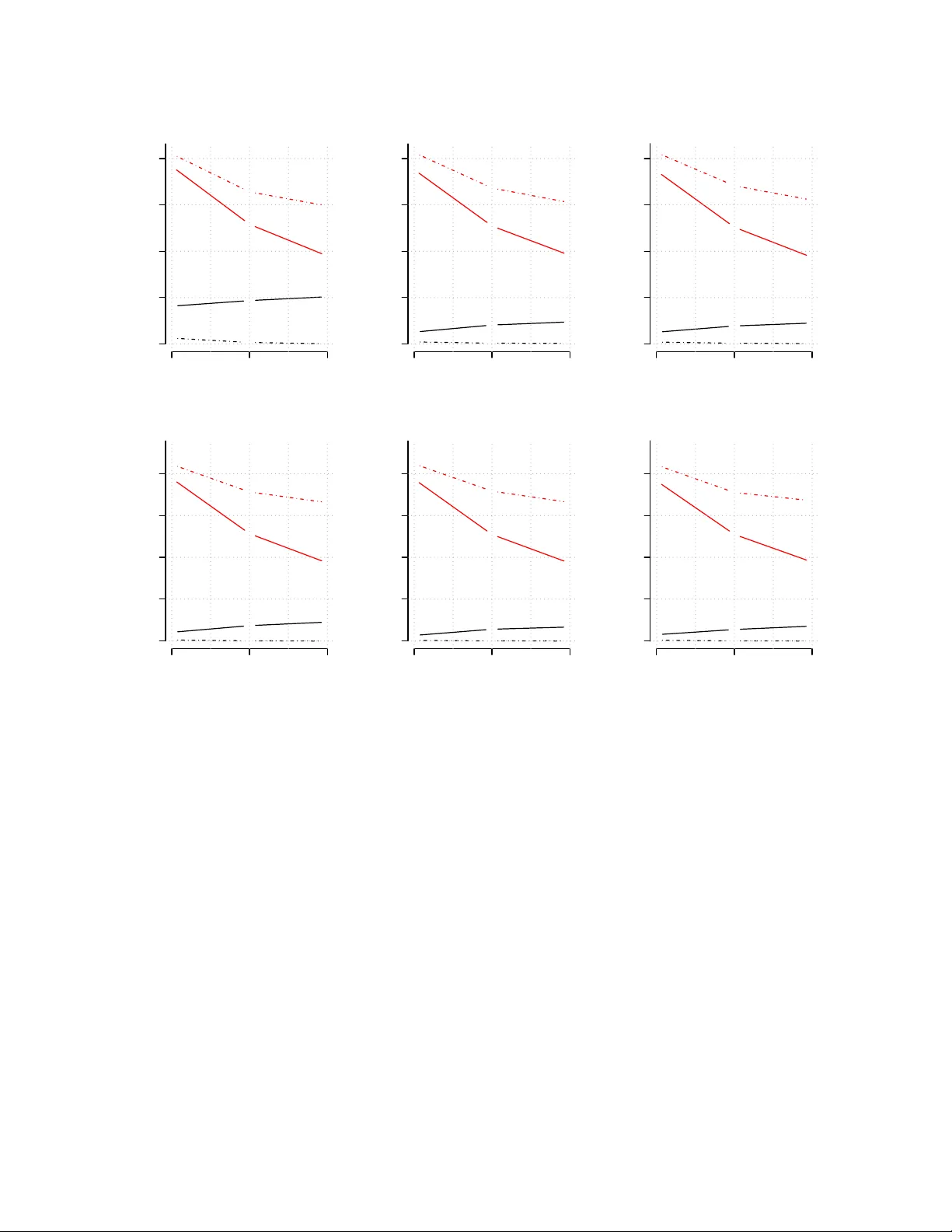
Online Up dating of Statistical Inference in the Big Data Setting Elizab eth D. Sc hifano, ∗ Departmen t of Statistics, Univ ersit y of Connecticut Jing W u, Departmen t of Statistics, Univ ersit y of Connecticut Ch un W ang, Departmen t of Statistics, Univ ersit y of Connecticut Jun Y an, Departmen t of Statistics, Univ ersit y of Connecticut and Ming-Hui Chen Departmen t of Statistics, Univ ersit y of Connecticut Ma y 26, 2015 Abstract W e present statistical methods for big data arising from online analytical pro cess- ing, where large amoun ts of data arriv e in streams and require fast analysis without storage/access to the historical data. In particular, w e develop iterative estimat- ing algorithms and statistical inferences for linear mo dels and estimating equations that up date as new data arriv e. These algorithms are computationally eﬃcient, minimally storage-in tensive, and allow for p ossible rank deﬁciencies in the subset design matrices due to rare-even t cov ariates. Within the linear mo del setting, the prop osed online-up dating framework leads to predictive residual tests that can b e used to assess the goo dness-of-ﬁt of the hypothesized mo del. W e also prop ose a new online-up dating estimator under the estimating equation setting. Theoretical prop- erties of the go o dness-of-ﬁt tests and prop osed estimators are examined in detail. In sim ulation studies and real data applications, our estimator compares fav orably with comp eting approaches under the estimating equation setting. Keywor ds: data compression, data streams, estimating equations, linear regression mo dels ∗ P art of the computation was done on the Beo wulf cluster of the Department of Statistics, Universit y of Connecticut, partially ﬁnanced by the NSF SCREMS (Scientiﬁc Computing Researc h Environmen ts for the Mathematical Sciences) gran t num ber 0723557. 1 1 In tro duction The adv ancement and prev alence of computer tec hnology in nearly every realm of science and daily life has enabled the collection of “big data”. While access to suc h wealth of information opens the do or tow ards new discov eries, it also p oses challenges to the curren t statistical and computational theory and metho dology , as well as c hallenges for data storage and computational eﬃciency . Recen t metho dological developmen ts in statistics that address the big data challenges ha v e largely fo cused on subsampling-based (e.g., Kleiner et al., 2014; Liang et al., 2013; Ma et al., 2013) and divide and conquer (e.g., Lin and Xi, 2011; Guha et al., 2012; Chen and Xie, 2014) tec hniques; see W ang et al. (2015) for a review. “Divide and conquer” (or “divide and recombine” or ‘split and conquer”, etc.), in particular, has b ecome a p opular approach for the analysis of large complex data. The approac h is appealing b ecause the data are ﬁrst divided into subsets and then n umeric and visualization metho ds are applied to eac h of the subsets separately . The divide and conquer approac h culminates b y aggregating the results from eac h subset to pro duce a ﬁnal solution. T o date, most of the fo cus in the ﬁnal aggregation step is in estimating the unkno wn quantit y of in terest, with little to no atten tion dev oted to standard error estimation and inference. In some applications, data arrives in streams or in large ch unks, and an online, sequen- tially up dated analysis is desirable without storage requiremen ts. As far as we are a w are, w e are the ﬁrst to examine inference in the online-up dating setting. Ev en with big data, inference remains an imp ortan t issue for statisticians, particularly in the presence of rare- ev en t co v ariates. In this work, w e pro vide standard error form ulae for divide-and-conquer estimators in the linear mo del (LM) and estimating equation (EE) framew ork. W e fur- ther dev elop iterative estimating algorithms and statistical inferences for the LM and EE framew orks for online-up dating, which up date as new data arrive. These algorithms are computationally eﬃcient, minimally storage-intensiv e, and allo w for possible rank deﬁcien- cies in the subset design matrices due to rare-ev en t co v ariates. Within the online-up dating setting for linear mo dels, we prop ose tests for outlier detection based on predictiv e residu- als and deriv e the exact distribution and the asymptotic distribution of the test statistics for the normal and non-normal cases, resp ectiv ely . In addition, within the online-updating 2 setting for estimating equations, w e prop ose a new estimator and sho w that it is asymptot- ically consisten t. W e further establish new uniqueness results for the resulting cum ulativ e EE estimators in the presence of rank-deﬁcient subset design matrices. Our simulation study and real data analysis demonstrate that the prop osed estimator outp erforms other divide-and-conquer or online-up dated estimators in terms of bias and mean squared error. The manuscript is organized as follo ws. In Section 2, we ﬁrst brieﬂy review the divide- and-conquer approach for linear regression mo dels and introduce formulae to compute the mean square error. W e then present the linear mo del online-up dating algorithm, address p ossible rank deﬁciencies within subsets, and propose predictive residual diagnostic tests. In Section 3, w e review the divide-and-conquer approac h of Lin and Xi (2011) for estimating equations and introduce corresp onding v ariance form ulae for the estimators. W e then build up on this divide-and-conquer strategy to derive our online-up dating algorithm and new online-up dated estimator. W e further provide theoretical results for the new online- up dated estimator and address possible rank deﬁciencies within subsets. Section 4 con tains our n umerical simulation results for b oth the LM and EE settings, while Section 5 contains results from the analysis of real data regarding airline on-time statistics. W e conclude with a brief discussion. 2 Normal Linear Regression Mo del 2.1 Notation and Preliminaries Supp ose there are N indep enden t observ ations { ( y i , x i ) , i = 1 , 2 , . . . , N } of in terest and we wish to ﬁt a normal linear regression model y i = x 0 i β +  i , where  i ∼ N (0 , σ 2 ) independently for i = 1 , 2 , . . . , N , and β is a p -dimensional vector of regression co eﬃcien ts corresp onding to cov ariates x i ( p × 1). W rite y = ( y 1 , y 2 , . . . , y N ) 0 and X = ( x 1 , x 2 , . . . , x N ) 0 where we assume the design matrix X is of full rank p < N . The least squares (LS) estimate of β and the corresp onding residual mean square, or mean squared error (MSE), are giv en b y ˆ β = ( X 0 X ) − 1 X 0 y and MSE = 1 N − p y 0 ( I N − H ) y , resp ectively , where I N is the N × N iden tit y matrix and H = X ( X 0 X ) − 1 X 0 . In the online-up dating setting, w e supp ose that the N observ ations are not av ailable all 3 at once, but rather arriv e in ch unks from a large data stream. Suppose at eac h accumulation p oin t k we observe y k and X k , the n k -dimensional v ector of resp onses and the n k × p matrix of co v ariates, resp ectiv ely , for k = 1 , . . . , K suc h that y = ( y 0 1 , y 0 2 , . . . , y 0 K ) 0 and X = ( X 0 1 , X 0 2 , . . . , X 0 K ) 0 . Pro vided X k is of full rank, the LS estimate of β based on the k th subset is giv en by ˆ β n k ,k = ( X 0 k X k ) − 1 X 0 k y k (1) and the MSE is giv en b y MSE n k ,k = 1 n k − p y 0 k ( I n k − H k ) y k , (2) where H k = X k ( X 0 k X k ) − 1 X 0 k , for k = 1 , 2 , . . . , K . As in the divide-and-conquer approac h (e.g., Lin and Xi, 2011), we can write ˆ β as ˆ β =  K X k =1 X 0 k X k  − 1 K X k =1 X 0 k X k ˆ β n k ,k . (3) W e provide a similar divide-and-conquer expression for the residual sum of squares, or sum of squared errors (SSE), giv en b y SSE = K X k =1 y 0 k y k −  K X k =1 X 0 k X k ˆ β n k ,k  0  K X k =1 X 0 k X k  − 1  K X k =1 X 0 k X k ˆ β n k ,k  , (4) and MSE = SSE / ( N − p ) . The SSE, written as in (4), is quite useful if one is in terested in p erforming inference in the divide-and-conquer setting, as v ar( ˆ β ) may b e estimated b y MSE( X 0 X ) − 1 = MSE  P K k =1 X 0 k X k  − 1 . W e will see in Section 2.2 that b oth ˆ β in (3) and SSE in (4) ma y b e expressed in sequential form that is more adv antageous from the p ersp ectiv e of online-up dating. 2.2 Online Up dating While equations (3) and (4) are quite amenable to parallel pro cessing for each subset, the online-up dating approac h for data streams is inheren tly sequen tial in nature. Equations (3) and (4) can certainly be used for estimation and inference for regression co eﬃcien ts resulting at some terminal p oin t K from a data stream, pro vided quantities ( X 0 k X k , ˆ β n k ,k , y 0 k y k ) are a v ailable for all accumulation p oints k = 1 , . . . , K. How ever, suc h data storage ma y not 4 alw a ys be p ossible or desirable. F urthermore, it ma y also be of in terest to perform inference at a given accumulation step k , using the k subsets of data observed to that point. Th us, our ob jective is to form ulate a computationally eﬃcient and minimally storage-intensiv e pro cedure that will allow for online-up dating of estimation and inference. 2.2.1 Online Up dating of LS Estimates While our ultimate estimation and inferen tial pro cedures are frequentist in nature, a Ba y esian p ersp ectiv e provides some insigh t into ho w w e may construct our online-up dating estimators. Under a Ba yesian framew ork, using the previous k − 1 subsets of data to construct a prior distribution for the current data in subset k , we immediate iden tify the appropriate online up dating form ulae for estimating the regression co eﬃcients β and the error v ariance σ 2 with eac h new incoming dataset ( y k , X k ). The Bay esian paradigm and accompan ying form ulae are provided in the Supplemen tary Material. Let ˆ β k and MSE k denote the LS estimate of β and the corresp onding MSE based on the cumulativ e data D k = { ( y ` , X ` ) , ` = 1 , 2 , . . . , k } . The online-up dated estimator of β based on cum ulativ e data D k is given by ˆ β k = ( X 0 k X k + V k − 1 ) − 1 ( X 0 k X k ˆ β n k k + V k − 1 ˆ β k − 1 ) , (5) where ˆ β 0 = 0 , ˆ β n k k is deﬁned b y (1) or (7), V k = P k ` =1 X 0 ` X ` for k = 1 , 2 , . . . , and V 0 = 0 p is a p × p matrix of zeros. Although motiv ated through Ba y esian argumen ts, (5) ma y also b e found in a (non-Bay esian) recursive linear mo del framew ork (e.g., Stengel, 2012, page 313). The online-up dated estimator of the SSE based on cum ulative data D k is given by SSE k = SSE k − 1 + SSE n k ,k + ˆ β 0 k − 1 V k − 1 ˆ β k − 1 + ˆ β 0 n k ,k X 0 k X k ˆ β n k ,k − ˆ β 0 k V k ˆ β k (6) where SSE n k ,k is the residual sum of squares from the k th dataset, with corresp onding residual mean square MSE n k ,k =SSE n k ,k / ( n k − p ) . The MSE based on the data D k is then MSE k = SSE k / ( N k − p ) where N k = P k ` =1 n ` (= n k + N k − 1 ) for k = 1 , 2 , . . . . Note that for k = K , equations (5) and (6) are iden tical to those in (3) and (4), resp ectiv ely . Notice that, in addition to quan tities only in volving the current data ( y k , X k ) (i.e., ˆ β n k ,k , SSE n k ,k , X 0 k X k , and n k ), w e only used quan tities ( ˆ β k − 1 , SSE k − 1 , V k − 1 , N k − 1 ) from 5 the previous accum ulation p oint to compute ˆ β k and MSE k . Based on these online-up dated estimates, one can easily obtain online-up dated t-tests for the regression parameter esti- mates. Online-up dated ANOV A tables require storage of t wo additional scalar quantities from the previous accum ulation p oint; details are pro vided in the Supplementary Material. 2.2.2 Rank Deﬁciencies in X k When dealing with subsets of data, either in the divide-and-conquer or the online-up dating setting, it is quite p ossible (e.g., in the presence of rare ev en t co v ariates) that some of the design matrix subsets X k will not be of full rank, even if the design matrix X for the entire dataset is of full rank. F or a giv en subset k , note that if the columns of X k are not linearly indep enden t, but lie in a space of dimension q k < p , the estimate ˆ β n k ,k = ( X 0 k X k ) − X 0 k y k , (7) where ( X 0 k X k ) − is a generalized in verse of ( X 0 k X k ) for subset k , will not b e unique. Ho wev er, b oth ˆ β and MSE will be unique, which leads us to in tro duce the follo wing proposition. Prop osition 2.1 Supp ose X is of ful l r ank p < N . If the c olumns of X k ar e not line arly indep endent, but lie in a sp ac e of dimension q k < p for any k = 1 , . . . , K , ˆ β in (3) and SSE (4) using ˆ β n k ,k as in (7) wil l b e invariant to the choic e of gener alize d inverse ( X 0 k X k ) − of ( X 0 k X k ) . T o see this, recall that a generalized inv erse of a matrix B , denoted b y B − , is a matrix suc h that BB − B = B . Note that for ( X 0 k X k ) − , a generalized inv erse of ( X 0 k X k ) , ˆ β n k ,k giv en in (7) is a solution to the linear system ( X 0 k X k ) β k = X 0 k y k . It is w ell known that if ( X 0 k X k ) − is a generalized inv erse of ( X 0 k X k ) , then X k ( X 0 k X k ) − X 0 k is inv ariant to the c hoice of ( X 0 k X k ) − (e.g., Searle, 1971, p20). Both (3) and (4) rely on ˆ β n k ,k only through product X 0 k X k ˆ β n k ,k = X 0 k X k ( X 0 k X k ) − X 0 k y k = X 0 k y k whic h is in v arian t to the c hoice of ( X 0 k X k ) − . Remark 2.2 The o nline-up dating formulae (5) and (6) do not r e quir e X 0 k X k for al l k to b e invertible. In p articular, the online-up dating scheme only r e quir es V k = P k ` =1 X 0 ` X ` to b e invertible. This fact c an b e made mor e explicit by r ewriting (5) and (6) , r esp e ctively, as ˆ β k = ( X 0 k X k + V k − 1 ) − 1 ( X 0 k y k + W k − 1 ) = V − 1 k ( X 0 k y k + W k − 1 ) (8) SSE k = SSE k − 1 + y 0 k y k + ˆ β 0 k − 1 V k − 1 ˆ β k − 1 − ˆ β 0 k V k ˆ β k (9) 6 wher e W 0 = 0 and W k = P k ` =1 X 0 ` y ` for k = 1 , 2 , . . . . Remark 2.3 F ol lowing R emark 2.2 and using the Bayesian motivation discusse d in the Supplementary Material, if X 1 is not of ful l r ank (e.g., due to a r ar e event c ovariate), we may c onsider a r e gularize d le ast squar es estimator by setting V 0 6 = 0 p . F or example, setting V 0 = λ I p , λ > 0 , with µ 0 = 0 would c orr esp ond to a ridge estimator and c ould b e use d at the b e ginning of the online estimation pr o c ess until enough data has ac cumulate d; onc e enough data has ac cumulate d, the biasing term V 0 = λ I p may b e r emove d such that the r emaining se quenc e of up date d estimators ˆ β k and MSE k ar e unbiase d for β and σ 2 , r esp e ctively. Mor e sp e ciﬁc al ly, set V k = P k ` =0 X 0 ` X ` (note that the summation starts at ` = 0 r ather than ` = 1 ) wher e X 0 0 X 0 ≡ V 0 , ke ep ˆ β 0 = 0 , and supp ose at ac cumulation p oint κ we have ac cumulate d enough data such that X κ is of ful l r ank. F or k < κ and V 0 = λ I p , λ > 0 , we obtain a (biase d) ridge estimator and c orr esp onding sum of squar e d err ors by using (5) and (6) or (8) and (9) . At k = κ , we c an r emove the bias with, e.g., ˆ β κ = ( X 0 κ X κ + V κ − 1 − V 0 ) − 1 ( X 0 κ y κ + W κ − 1 ) (10) SSE κ = SSE κ − 1 + y 0 κ y κ + ˆ β 0 κ − 1 V κ − 1 ˆ β κ − 1 − ˆ β 0 κ ( V κ − V 0 ) ˆ β κ , (11) and then pr o c e e d with original up dating pr o c e dur e for k > κ to obtain unbiase d estimators of β and σ 2 . 2.3 Mo del Fit Diagnostics While the adv antages of sa ving only lo wer-dimensional summaries are clear, a potential dis- adv an tage arises in terms of diﬃcult y performing classical residual-based mo del diagnostics. Since we hav e not sa ved the individual observ ations from the previous ( k − 1) datasets, w e can only compute residuals based up on the current observ ations ( y k , X k ) . F or example, one may compute the residuals e ki = y ki − ˆ y ki , where i = 1 , . . . , n k and ˆ y ki = x 0 ki ˆ β n k ,k , or ev en the externally studentized residuals giv en b y t ki = e ki p MSE n k ,k ( i ) (1 − h k,ii ) = e ki h n k − p − 1 SSE n k ,k (1 − h k,ii ) − e 2 ki i 1 / 2 , (12) where h k,ii = Diag( H k ) i = Diag( X k ( X 0 k X k ) X 0 k ) i and MSE n k ,k ( i ) is the MSE computed from the k th subset with the i th observ ation remov ed, i = 1 , . . . , n k . 7 Ho w ever, for mo del ﬁt diagnostics in the online-up date setting, it would arguably b e more useful to consider the pr e dictive r esiduals , based on ˆ β k − 1 from data D k − 1 with pre- dicted v alues ˇ y k = ( ˇ y k 1 , . . . , ˇ y kn k ) 0 = X k ˆ β k − 1 , as ˇ e ki = y ki − ˇ y ki , i = 1 , . . . , n k . Deﬁne the standardized predictive residuals as ˇ t ki = ˇ e ki / p ˆ v ar( ˇ e ki ) , i = 1 , . . . , n k . (13) 2.3.1 Distribution of standardized predictive residuals T o derive the distribution of ˇ t ki , we in tro duce new notation. Denote y k − 1 = ( y 0 1 , . . . , y 0 k − 1 ) 0 , and X k − 1 and ε k − 1 the corresponding N k − 1 × p design matrix of stac ked X ` , ` = 1 , . . . , k − 1 , and N k − 1 × 1 random errors, respectively . F or new observ ations y k , X k , we assume y k = X k β +  k , (14) where the elemen ts of  k are indep enden t with mean 0 and v ariance σ 2 indep enden tly of the elemen ts of ε k − 1 whic h also ha ve mean 0 and v ariance σ 2 . Th us, E ( ˇ e ki ) = 0 , v ar( ˇ e ki ) = σ 2 (1 + x 0 ki ( X 0 k − 1 X k − 1 ) − 1 x ki ) for i = 1 , . . . , n k , and v ar( ˇ e k ) = σ 2 ( I n k + X k ( X 0 k − 1 X k − 1 ) − 1 X 0 k ) where ˇ e k = ( ˇ e k 1 , . . . , ˇ e kn k ) 0 . If w e assume that both  k and ε k − 1 are normally distributed, then it is easy to sho w that ˇ e 0 k v ar( ˇ e k ) − 1 ˇ e k ∼ χ 2 n k . Thus, estimating σ 2 with MSE k − 1 and noting that N k − 1 − p σ 2 MSE k − 1 ∼ χ 2 N k − 1 − p indep enden tly of ˇ e 0 k v ar( ˇ e k ) − 1 ˇ e k , we ﬁnd that ˇ t ki ∼ t N k − 1 − p and ˇ F k := ˇ e 0 k ( I n k + X k ( X 0 k − 1 X k − 1 ) − 1 X 0 k ) − 1 ˇ e k n k MSE k − 1 ∼ F n k ,N k − 1 − p . (15) If w e are not willing to assume normalit y of the errors, w e in tro duce the follo wing prop o- sition. The proof of the prop osition is giv en in the Supplemen tary Material. Prop osition 2.4 Assume that 1.  i , i = 1 , . . . , n k , ar e indep endent and identic al ly distribute d with E (  i ) = 0 and E (  2 i ) = σ 2 ; 8 2. the elements of the design matrix X k ar e uniformly b ounde d, i.e., | X ij | < C , ∀ i, j , wher e C < ∞ is c onstant; 3. lim N k − 1 →∞ X 0 k − 1 X k − 1 N k − 1 = Q , wher e Q is a p ositive deﬁnite matrix. L et ˇ e ∗ k = Γ − 1 ˇ e k , wher e ΓΓ 0 , I n k + X k ( X 0 k − 1 X k − 1 ) − 1 X 0 k . Write ˇ e ∗ k 0 = ( ˇ e ∗ k 1 0 , . . . , ˇ e ∗ k m 0 ) , wher e ˇ e ∗ k i is an n k i × 1 ve ctor c onsisting of the ( P i − 1 ` =1 n k ` + 1) th c omp onent thr ough the ( P i ` =1 n k ` ) th c omp onent of ˇ e ∗ k , and P m i =1 n k i = n k . We further assume that 4. lim n k →∞ n k i n k = C i , wher e 0 < C i < ∞ is c onstant for i = 1 , . . . , m . Then at ac cumulation p oint k , we have P m i =1 1 n k i ( 1 0 k i ˇ e ∗ k i ) 2 MSE k − 1 d − → χ 2 m , as n k , N k − 1 → ∞ , (16) wher e 1 k i is an n k i × 1 ve ctor of al l ones. 2.3.2 T ests for Outliers Under normalit y of the random errors, we ma y use statistics ˇ t ki in (13) and ˇ F k in (15) to test individually or globally if there are any outliers in the k th dataset. Notice that ˇ t ki in (13) and ˇ F k in (15) can b e re-expressed equiv alen tly as ˇ t ki = ˇ e ki / q MSE k − 1 (1 + x 0 ki ( V k − 1 ) − 1 x ki ) (17) ˇ F k = ˇ e 0 k ( I n k + X k ( V k − 1 ) − 1 X 0 k ) − 1 ˇ e k n k MSE k − 1 (18) and th us can b oth b e computed with the lo wer-dimensional stored summary statistics from the previous accum ulation p oint. W e ma y iden tify as outlying y ki observ ations those cases whose standardized predicted ˇ t ki are large in magnitude. If the regression model is appropriate, so that no case is outlying b ecause of a change in the mo del, then eac h ˇ t ki will follow the t distribution with N k − 1 − p degrees of freedom. Let p ki = P ( | t N k − 1 − p | > | ˇ t ki | ) b e the unadjusted p -v alue and let ˜ p ki b e the corresp onding adjuste d p -v alue for m ultiple testing (e.g., Benjamini and Ho c hberg, 1995; Benjamini and Y ekutieli, 2001). W e will declare y ki an outlier if ˜ p ki < α for a presp eciﬁed α lev el. Note that while the Benjamini-Ho c h b erg pro cedure assumes the 9 m ultiple tests to b e indep endent or p ositively correlated, the predictive residuals will b e appro ximately indep enden t as the sample size increases. Th us, we w ould exp ect the false disco v ery rate to b e con trolled with the Benjamini-Ho c hberg p -v alue adjustmen t for large N k − 1 . T o test if there is at least one outlying v alue based upon n ull h yp othesis H 0 : E ( ˇ e k ) = 0 , w e will use statistic ˇ F k . V alues of the test statistic larger than F (1 − α, n k , N k − 1 − p ) w ould indicate at least one outlying y ki exists among i = 1 , . . . , n k at the corresp onding α lev el. If w e are un willing to assume normalit y of the random errors, we ma y still p erform a global outlier test under the assumptions of Prop osition 2.4. Using Prop osition 2.4 and follo wing the calibration proposed in Muirhead (1982) (Muirhead, 2009, page 218), we obtain an asymptotic F statistic ˇ F a k := P m i =1 1 n k i ( 1 0 k i ˇ e ∗ k i ) 2 MSE k − 1 N k − 1 − m + 1 N k − 1 · m d − → F ( m, N k − 1 − m + 1) , as n k , N k − 1 → ∞ . (19) V alues of the test statistic ˇ F a k larger than F (1 − α, m, N k − 1 − m + 1) would indicate at least one outlying observ ation exists among y k at the corresp onding α lev el. Remark 2.5 R e c al l that var ( ˇ e k ) = ( I n k + X k ( X 0 k − 1 X k − 1 ) − 1 X 0 k ) σ 2 , ΓΓ 0 σ 2 , wher e Γ is an n k × n k invertible matrix. F or lar ge n k , it may b e chal lenging to c ompute the Cholesky de c omp osition of var ( ˇ e k ) . One p ossible solution that avoids the lar ge n k issue is given in the Supplementary Material. 3 Online Up dating for Estimating Equations A nice prop ert y in the normal linear regression mo del setting is that regardless of whether one “divides and conquers” or p erforms online up dating, the ﬁnal solution ˆ β K will be the same as it would ha ve b een if one could ﬁt all of the data sim ultaneously and obtained ˆ β directly . Ho w ever, with generalized linear mo dels and estimating equations, this is t ypically not the case, as the score or estimating functions are often nonlinear in β . Consequen tly , divide and conquer strategies in these settings often rely on some form of linear approx- imation to attempt to conv ert the estimating equation problem into a least square-t yp e problem. F or example, follo wing Lin and Xi (2011), supp ose N indep enden t observ ations 10 { z i , i = 1 , 2 , . . . , N } . F or generalized linear mo dels, z i will b e ( y i , x i ) pairs, i = 1 , . . . , N with E ( y i ) = g ( x 0 i β ) for some kno wn function g . Supp ose there exists β 0 ∈ R p suc h that P N i =1 E [ ψ ( z i , β 0 )] = 0 for some score or estimating function ψ . Let ˆ β N denote the solution to the estimating equation (EE) M ( β ) = N X i =1 ψ ( z i , β ) = 0 and let ˆ V N b e its corresponding estimate of co v ariance, often of sandwich form. Let { z ki , i = 1 , . . . , n k } be the observ ations in the k th subset. The estimating function for subset k is M n k ,k ( β ) = n k X i =1 ψ ( z ki , β ) . (20) Denote the solution to M n k ,k ( β ) = 0 as ˆ β n k ,k . If w e deﬁne A n k ,k = − n k X i =1 ∂ ψ ( z ki , ˆ β n k ,k ) ∂ β , (21) a T aylor Expansion of − M n k ,k ( β ) at ˆ β n k ,k is given by − M n k ,k ( β ) = A n k ,k ( β − ˆ β n k ,k ) + R n k ,k as M n k ,k ( ˆ β n k ,k ) = 0 and R n k ,k is the remainder term. As in the linear mo del case, w e do not require A n k ,k to b e inv ertible for each subset k , but do require that P k ` =1 A n ` ,` is in v ertible. Note that for the asymptotic theory in Section 3.3, w e assume that A n k ,k is in v ertible for large n k . F or ease of notation, we will assume for no w that each A n k ,k is in v ertible, and w e will address rank deﬁcien t A n k ,k in Section 3.4 b elow. The aggregated estimating equation (AEE) estimator of Lin and Xi (2011) combines the subset estimators through ˆ β N K = K X k =1 A n k ,k ! − 1 K X k =1 A n k ,k ˆ β n k ,k (22) whic h is the solution to P K k =1 A n k ,k ( β − ˆ β n k ,k ) = 0 . Lin and Xi (2011) did not discuss a v ariance formula, but a natural v ariance estimator is given by ˆ V N K = K X k =1 A n k ,k ! − 1 K X k =1 A n k ,k ˆ V n k ,k A > n k ,k   K X k =1 A n k ,k ! − 1   > , (23) 11 where ˆ V n k ,k is the v ariance estimator of ˆ β n k ,k from the subset k . If ˆ V n k ,k is of sandwic h form, it can b e expressed as A − 1 n k ,k ˆ Q n k ,k A − 1 n k ,k , where ˆ Q n k ,k is an estimate of Q n k ,k = v ar( M n k ,k ( β )). Then, the v ariance estimator b ecomes ˆ V N K = K X k =1 A n k ,k ! − 1 K X k =1 ˆ Q n k ,k   K X k =1 A n k ,k ! − 1   > , (24) whic h is still of sandwic h form. 3.1 Online Up dating No w consider the online-up dating p ersp ectiv e in whic h w e would lik e to up date the es- timates of β and its v ariance as new data arrives. F or this purp ose, we introduce the cum ulativ e estimating equation (CEE) estimator for the regression co eﬃcien t v ector at accum ulation point k as ˆ β k = ( A k − 1 + A n k ,k ) − 1 ( A k − 1 ˆ β k − 1 + A n k ,k ˆ β n k ,k ) . (25) for k = 1 , 2 , . . . where ˆ β 0 = 0 , A 0 = 0 p , and A k = P k ` =1 A n ` ,` = A k − 1 + A n k ,k . F or the v ariance estimator at the k th up date, we tak e ˆ V k = ( A k − 1 + A n k ,k ) − 1 ( A k − 1 ˆ V k − 1 A > k − 1 + A n k ,k ˆ V n k ,k A > n k ,k )[( A k − 1 + A n k ,k ) − 1 ] > , (26) with ˆ V 0 = 0 p and A 0 = 0 p . By induction, it can b e sho wn that (25) is equiv alent to the AEE com bination (22) when k = K , and likewise (26) is equiv alent to (24) (i.e., AEE=CEE). Ho wev er, the AEE estimators, and consequently the CEE estimators, are not identical to the EE estimators ˆ β N and ˆ V N based on all N observ ations. It should b e noted, ho wev er, that Lin and Xi (2011) did prov e asymptotic consistency of AEE estimator ˆ β N K under certain regularity conditions. Since the CEE estimators are not iden tical to the EE estimators in ﬁnite sample sizes, there is ro om for improv emen t. T ow ards this end, consider the T aylor expansion of − M n k ,k ( β ) around some v ector ˇ β n k ,k , to b e deﬁned later. Then − M n k ,k ( β ) = − M n k ,k ( ˇ β n k ,k ) + [ A n k ,k ( ˇ β n k ,k )]( β − ˇ β n k ,k ) + ˇ R n k ,k 12 with ˇ R n k ,k denoting the remainder. Denote ˜ β K as the solution of K X k =1 − M n k ,k ( ˇ β n k ,k ) + K X k =1 [ A n k ,k ( ˇ β n k ,k )]( β − ˇ β n k ,k ) = 0 . (27) Deﬁne ˜ A n k ,k = [ A n k ,k ( ˇ β n k ,k )] and assume A n k ,k refers to A n k ,k ( ˆ β n k ,k ) . Then w e hav e ˜ β K = ( K X k =1 ˜ A n k ,k ) − 1 ( K X k =1 ˜ A n k ,k ˇ β n k ,k + K X k =1 M n k ,k ( ˇ β n k ,k ) ) . (28) If we c ho ose ˇ β n k ,k = ˆ β n k ,k , then ˜ β K in (28) reduces to the AEE estimator of Lin and Xi (2011) in (22), as (27) reduces to P K k =1 A n k ,k ( β − ˆ β n k ,k ) = 0 b ecause M n k ,k ( ˆ β n k ,k ) = 0 for all k = 1 , . . . , K. How ever, one do es not need to choose ˇ β n k ,k = ˆ β n k ,k . In the online- up dating setting, at eac h accum ulation p oin t k , we hav e access to the summaries from the previous accum ulation p oin t k − 1 , so we may use this information to our adv antage when deﬁning ˇ β n k ,k . Consider the intermediary estimator given by ˇ β n k ,k = ( ˜ A k − 1 + A n k ,k ) − 1 ( k − 1 X ` =1 ˜ A n ` ,` ˇ β n ` ,` + A n k ,k ˆ β n k ,k ) (29) for k = 1 , 2 , . . . , ˜ A 0 = 0 p , ˇ β n 0 , 0 = 0 , and ˜ A k = P k ` =1 ˜ A n ` ,` . Estimator (29) com bines the previous intermediary estimators ˇ β n ` ,` , ` = 1 , . . . , k − 1 and the curren t subset estimator ˆ β n k ,k , and arises as the solution to the estimating equation k − 1 X ` =1 ˜ A n ` ,` ( β − ˇ β n ` ,` ) + A n k ,k ( β − ˆ β n k ,k ) = 0 , where A n k ,k ( β − ˆ β n k ,k ) serv es as a bias correction term due to the omission of − P k − 1 ` =1 M n k ,k ( ˇ β n k ,k ) from the equation. With the c hoice of ˇ β n k ,k as giv en in (29), w e introduce the cum ulatively up dated esti- mating equation (CUEE) estimator ˜ β k as ˜ β k = ( ˜ A k − 1 + ˜ A n k ,k ) − 1 ( a k − 1 + ˜ A n k ,k ˇ β n k ,k + b k − 1 + M n k ,k ( ˇ β n k ,k )) (30) with a k = P k ` =1 ˜ A n k ,k ˇ β n k ,k = ˜ A n k ,k ˇ β n k ,k + a k − 1 and b k = P k ` =1 M n k ,k ( ˇ β n k ,k ) = M n k ,k ( ˇ β n k ,k )+ b k − 1 where a 0 = b 0 = 0 , ˜ A 0 = 0 p , and k = 1 , 2 , . . . . Note that for a terminal k = K , (30) is equiv alent to (28). 13 F or the v ariance of ˜ β k , observe that 0 = − M n k ,k ( ˆ β n k ,k ) ≈ − M n k ,k ( ˇ β n k ,k ) + ˜ A n k ,k ( ˆ β n k ,k − ˇ β n k ,k ) . Th us, we ha v e ˜ A n k ,k ˇ β n k ,k + M n k ,k ( ˇ β n k ,k ) ≈ ˜ A n k ,k ˆ β n k ,k . Using the ab ov e approximation, the v ariance formula is giv en b y ˜ V k =( ˜ A k − 1 + ˜ A n k ,k ) − 1 ( k X ` =1 ˜ A n ` ,` ˆ V n ` ,` ˜ A > n ` ,` )[( ˜ A k − 1 + ˜ A n k ,k ) − 1 ] > =( ˜ A k − 1 + ˜ A n k ,k ) − 1 ( ˜ A k − 1 ˜ V k − 1 ˜ A > k − 1 + ˜ A n k ,k ˆ V n k ,k ˜ A > n k ,k )[( ˜ A k − 1 + ˜ A n k ,k ) − 1 ] > , (31) for k = 1 , 2 , . . . and ˜ A 0 = ˜ V 0 = 0 p . Remark 3.1 Under the normal line ar r e gr ession mo del, al l of the estimating e quation estimators b e c ome “exact”, in the sense that ˆ β N = ( X 0 X ) − 1 X 0 y = ˆ β N K = ˆ β K = ˜ β K . 3.2 Online Up dating for W ald T ests W ald tests ma y be used to test individual co eﬃcients or nested h yp otheses based upon ei- ther the CEE or CUEE estimators from the cum ulative data. Let ( ˘ β k = ( ˘ β k, 1 , . . . , ˘ β k,p ) 0 , ˘ V k ) refer to either the CEE regression coeﬃcien t estimator and corresp onding v ariance in equa- tions (25) and (26), or the CUEE regression co eﬃcien t estimator and corresp onding v ari- ance in equations (30) and (31). T o test H 0 : β j = 0 at the k th up date ( j = 1 , . . . , p ), we may tak e the W ald statis- tic z ∗ 2 k,j = ˘ β 2 k,j / v ar( ˘ β k,j ) , or equiv alen tly , z ∗ k,j = ˘ β k,j /se ( ˘ β k,j ) , where the standard error se ( ˘ β k,j ) = q v ar( ˘ β k,j ) and v ar( ˘ β k,j ) is the j th diagonal elemen t of ˘ V k . The corresp onding p-v alue is P ( | Z | ≥ | z ∗ k,j | ) = P ( χ 2 1 ≥ z ∗ 2 k,j ) where Z and χ 2 1 are standard normal and 1 degree-of-freedom chi-squared random v ariables, respectively . The W ald test statistic may also be used for assessing the diﬀerence b et w een a full mo del M1 relativ e to a nested submo del M2. If β is the parameter of mo del M1 and the nested submo del M2 is obtained from M1 b y setting C β = 0 , where C is a rank q contrast matrix and ˘ V is a consistent estimate of the co v ariance matrix of estimator ˘ β , the test statistic is ˘ β 0 C 0 ( C ˘ VC 0 ) − 1 C ˘ β , whic h is distributed as χ 2 q under the n ull hypothesis that C β = 0 . As an example, if M1 represents the full mo del con taining all p regression co eﬃcients at 14 the k th up date, where the ﬁrst co eﬃcien t β 1 is an intercept, we may test the global n ull h yp othesis H 0 : β 2 = . . . = β p = 0 with w ∗ k = ˘ β 0 k C 0 ( C ˘ V k C 0 ) − 1 C ˘ β k , where C is ( p − 1) × p matrix C = [ 0 , I p − 1 ] and the corresp onding p-v alue is P ( χ 2 p − 1 ≥ w ∗ k ) . 3.3 Asymptotic Results In this section, we sho w consistency of the CUEE estimator. Sp eciﬁcally , Theorem 3.2 sho ws that, under regularity , if the EE estimator based on the all N observ ations ˆ β N is a consisten t estimator and the partition num b er K go es to inﬁnity , but not to o fast, then the CUEE estimator ˜ β K is also a consisten t estimator. W e ﬁrst pro vide the tec hnical regularit y conditions. W e assume for simplicity of notation that n k = n for all k = 1 , 2 , . . . , K . Note that conditions (C1-C6) w ere giv en in Lin and Xi (2011), and are provided b elow for completeness. The proof of the theorem can be found in the Supplementary Material. (C1) The score function ψ is measurable for any ﬁxed β and is twice contin uously diﬀer- en tiable with resp ect to β . (C2) The matrix − ∂ ψ ( z i , β ) ∂ β is semi-p ositive deﬁnite (s.p.d.), and − P n i =1 ∂ ψ ( z i , β ) ∂ β is p ositive deﬁnite (p.d.) in a neigh b orho od of β 0 when n is large enough. (C3) The EE estimator ˆ β n,k is strongly consisten t, i.e. ˆ β n,k → β 0 almost surely (a.s.) as n → ∞ . (C4) There exists tw o p.d. matrices, Λ 1 and Λ 2 suc h that Λ 1 ≤ n − 1 A n,k ≤ Λ 2 for all k = 1 , . . . , K , i.e. for any v ∈ R p , v 0 Λ 1 v ≤ n − 1 v 0 A n,k v ≤ v 0 Λ 1 v , where A n,k is giv en in (21). (C5) In a neighborho o d of β 0 , the norm of the second-order deriv atives ∂ 2 ψ j ( z i , β ) ∂ β 2 is b ounded uniformly , i.e. k ∂ 2 ψ j ( z i , β ) ∂ β 2 k ≤ C 2 for all i, j , where C 2 is a constan t. (C6) There exists a real num b er α ∈ (1 / 4 , 1 / 2) suc h that for any η > 0, the EE estimator ˆ β n,k satisﬁes P ( n α k ˆ β n,k − β 0 k > η ) ≤ C η n 2 α − 1 , where C η > 0 is a constan t only dep ending on η . 15 Rather than using condition (C4), we will use a slightly mo diﬁed v ersion whic h fo cuses on the b eha vior of A n,k ( β ) for all β in the neighborho o d of β 0 (as in (C5)), rather than just at the subset estimate ˆ β n,k . (C4’) In a neighborho o d of β 0 , there exists tw o p.d. matrices Λ 1 and Λ 2 suc h that Λ 1 ≤ n − 1 A n,k ( β ) ≤ Λ 2 for all β in the neighborho o d of β 0 and for all k = 1 , ..., K . Theorem 3.2 L et ˆ β N b e the EE estimator b ase d on entir e data. Then under (C1)-(C2), (C4’)-(C6), if the p artition numb er K satisﬁes K = O ( n γ ) for some 0 < γ < min { 1 − 2 α, 4 α − 1 } , we have P ( √ N k ˜ β K − ˆ β N k > δ ) = o (1) for any δ > 0 . Remark 3.3 If n k 6 = n for al l k , The or em 3.2 wil l stil l hold, pr ovide d for e ach k , n k − 1 n k is b ounde d, wher e n k − 1 and n k ar e the r esp e ctive sample sizes for subsets k − 1 and k . Remark 3.4 Supp ose N indep endent observations ( y i , x i ) , i = 1 , . . . , N , wher e y is a sc alar r esp onse and x is a p -dimensional ve ctor of pr e dictor variables. F urther supp ose E ( y i ) = g ( x 0 i β ) for i = 1 , . . . , N for g a c ontinuously diﬀer entiable function. Under mild r e gularity c onditions, Lin and Xi (2011) show in their The or em 5.1 that c ondition (C6) is satisﬁe d for a simpliﬁe d version of the quasi-likeliho o d estimator of β (Chen et al., 1999), given as the solution to the estimating e quation Q ( β ) = N X i =1 [ y i − g ( x 0 i β )] x i = 0 . 3.4 Rank Deﬁciencies in X k Supp ose N indep endent observ ations ( y i , x i ) , i = 1 , . . . , N , where y is a scalar response and x is a p -dimensional vector of predictor v ariables. Using the same notation from the linear mo del setting, let ( y ki , x ki ) , i = 1 , . . . , n k , b e the observ ations from the k th subset where y k = ( y k 1 , y k 2 , . . . , y kn k ) 0 and X k = ( x k 1 , x k 2 , . . . , x kn k ) 0 . F or subsets k in whic h X k is not of full rank, w e may ha ve diﬃcult y in solving the subset EE to obtain ˆ β n k ,k , which is used to compute b oth the AEE/CEE and CUEE estimators for β in (22) and (28), resp ectiv ely . Ho w ever, just as in the linear mo del case, w e can show under certain conditions that if X = ( X 0 1 , X 0 2 , . . . , X 0 K ) 0 has full column rank p , then the estimators ˆ β N K in (22) and ˜ β K in (28) for some terminal K will b e unique. 16 Sp eciﬁcally , consider observ ations ( y k , X k ) suc h that E ( y ki ) = µ ki = g ( η ki ) with η ki = x 0 ki β for some kno wn function g . The estimating function ψ for the k th dataset is of the form ψ ( z ki , β ) = x ki S ki W ki ( y ki − µ ki ) , i = 1 , . . . , n k , where S ki = ∂ µ ki /∂ η ki , and W ki is a positive and p ossibly data dependent weigh t. Sp ecif- ically , W ki ma y depend on β only through η ki . In matrix form, the estimating equation b ecomes X 0 k S 0 k W k ( y k − µ k ) = 0 , (32) where S k = Diag( S k 1 , . . . , S kn k ), W k = Diag( W k 1 , . . . , W kn k ), and µ k =  µ k 1 , . . . , µ kn k  0 . With S k , W k , and µ k ev aluated at some initial v alue β (0) , the standard Newton– Raphson metho d for the iterativ e solution of (32) solv es the linear equations X 0 k S 0 k W k S k X k ( β − β (0) ) = X 0 k S 0 k W k ( y k − µ k ) (33) for an up dated β . Rewrite equation (33) as X 0 k S 0 k W k S k X k β = X 0 k S 0 k W k v k (34) where v k = y k − µ k + S k X k β (0) . Equation (34) is the normal equation of a w eighted least squares regression with resp onse v k , design matrix S k X k , and weigh t W k . Therefore the iterativ e rew eighted least squares approach (IRLS) can b e used to implement the Newton– Raphson metho d for an iterativ e solution to (32) (e.g., Green, 1984). Rank deﬁciency in X k calls for a generalized inv erse of X 0 k S 0 k W k S k X k . In order to sho w uniqueness of estimators ˆ β N K in (22) and ˜ β K in (28) for some terminal K , w e must ﬁrst establish that the IRLS algorithm will work and conv erge for subset k given the same initial v alue β (0) when X k is not of full rank. Upon con v ergence of IRLS at subset k with solution ˆ β n k ,k , we must then v erify that the CEE and CUEE estimators that rely on ˆ β n k ,k are unique. The follo wing prop osition summarizes the result; the pro of is pro vided in the Supplemen tary Material. 17 Prop osition 3.5 Under the ab ove formulation, assuming that c onditions (C1-C3) hold for a ful l-r ank sub-c olumn matrix of X k , estimators ˆ β N K in (22) and ˜ β K in (28) for some terminal K wil l b e unique pr ovide d X is of ful l r ank. The simulations in Section 4.2 consider rank deﬁciencies in binary logistic regression and P oisson regression. Note that for these mo dels, the v ariance of the estimators ˆ β K and ˜ β K are giv en by A − 1 K = ( P K k =1 A n k ,k ) − 1 or ˜ A − 1 K = ( P K k =1 ˜ A n k ,k ) − 1 . F or robust sandwich estimators, for those subsets k in which A n k ,k is not inv ertible, we replace A n k ,k ˆ V n k ,k A > n k ,k and ˜ A n k ,k ˆ V n k ,k ˜ A > n k ,k in the “meat” of equations (26) and (31), resp ectiv ely , with an es- timate of Q n k ,k from (24). In particular, w e use ˆ Q n k ,k = P n k i =1 ψ ( z ki , ˆ β k ) ψ ( z ki , ˆ β k ) > for the CEE v ariance and ˜ Q n k ,k = P n k i =1 ψ ( z ki , ˜ β k ) ψ ( z ki , ˜ β k ) > for the CUEE v ariance. W e use these mo diﬁcations in the robust Poisson regression simulations in Section 4.2.2 for the CEE and CUEE estimators, as by design, we include binary cov ariates with somewhat lo w success probabilities. Consequently , not all subsets k will observ e b oth successes and failures, particularly for co v ariates with success probabilities of 0.1 or 0.01, and the corre- sp onding design matrices X k will not alw a ys b e of full rank. Th us A n k ,k will not alw a ys b e in v ertible for ﬁnite n k , but will b e in v ertible for large enough n k . W e also p erform pro of of concept simulations in Section 4.2.3 in binary logistic regression, where we compare CUEE estimators under diﬀeren t choices of generalized inv erses. 4 Sim ulations 4.1 Normal Linear Regression: Residual Diagnostic P erformance In this section w e ev aluate the p erformance of the outlier tests discussed in Section 2.3.2. Let k ∗ denote the index of the single subset of data con taining an y outliers. W e generated the data according to the mo del y ki = x 0 ki β +  ki + b k δ η ki , i = 1 , . . . , n k , (35) where b k = 0 if k 6 = k ∗ and b k ∼ Bernoulli(0 . 05) otherwise. Notice that the ﬁrst tw o terms on the right-hand-side correspond to the usual linear mo del with β = (1 , 2 , 3 , 4 , 5) 0 , x ki [2:5] ∼ N ( 0 , I 4 ) indep enden tly , x ki [1] = 1, and  ki are the indep enden t errors, while the 18 ﬁnal term is resp onsible for generating the outliers. Here, η ki ∼ Exp(1) indep enden tly and δ is the scale parameter con trolling magnitude or strength of the outliers. W e set δ ∈ { 0 , 2 , 4 , 6 } corresponding to “no”, “small”, “medium”, and “large” outliers. T o ev aluate the p erformance of the individual outlier test in (17), w e generated the random errors as  ki ∼ N(0 , 1) . T o ev aluate the p erformance of the global outlier tests in (18) and (19), we additionally considered  ki as indep enden t skew-t v ariates with degrees of freedom ν = 3 and skewing parameter γ = 1 . 5, standardized to ha ve mean 0 and v ariance 1. T o be precise, we use the sk ew t densit y g ( x ) =    2 γ + 1 γ f ( γ x ) for x < 0 2 γ + 1 γ f ( x γ ) for x ≥ 0 where f ( x ) is the density of the t distribution with ν degrees of freedom. F or all outlier simulations, we v aried k ∗ , the lo cation along the data stream in which the outliers occur. W e also v aried n k = n k ∗ ∈ { 100 , 500 } whic h additionally con trols the n umber of outliers in dataset k ∗ . F or eac h subset ` = 1 , . . . , k ∗ − 1 and for 95% of observ ations in subset k ∗ , the data did not contain an y other outliers. T o ev aluate the global outlier tests (18) and (19) with m = 2, we estimated p ow er using B = 500 sim ulated data sets with signiﬁcance level α = 0 . 05 , where pow er was estimated as the proportion of 500 datasets in whic h ˇ F k ∗ ≥ F (0 . 95 , n k ∗ , N k ∗ − 1 − 5) or ˇ F a k ∗ ≥ F (0 . 95 , 2 , N k ∗ − 1 − 1) . The p ow er estimates for the v arious subset sample sizes n k ∗ , lo cations of outliers k ∗ , and outlier strengths δ app ear in T able 1. When the errors were normally distributed (top portion of table), notice that the T yp e I error rate w as controlled in all scenarios for b oth the F test and asymptotic F test. As exp ected, p o w er tends to increase as outlier strength and/or the n um b er of outliers increase. F urthermore, larger v alues of k ∗ , and hence greater prop ortions of “go o d” outlier-free data, also tend to ha ve higher p o wer; ho wev er, the magnitude of improv ement decreases once the denominator degrees of freedom ( N k ∗ − 1 − p or N k ∗ − 1 − m + 1) b ecome large enough, and the F tests essen tially reduce to χ 2 tests. Also as exp ected, the F test giv en b y (18) is more p o w erful than the asymptotic F test giv en in (19) when, in fact, the errors w ere normally distributed. When the errors were not normally distributed (b ottom portion of table), the empirical t yp e I error rates of the F test giv en b y (18) are sev erely inﬂated and hence, its empirical 19 T able 1: P ow er of the outlier tests for v arious lo cations of outliers ( k ∗ ), subset sample sizes ( n k = n k ∗ ), and outlier strengths (no, small, medium, large). Within each cell, the top en try corresp onds to the normal-based F test and the b ottom en try corresponds to the asymptotic F test that does not rely on normality of the errors. Outlier n k ∗ = 100 (5 true outliers) n k ∗ = 500 (25 true outliers) Strength k ∗ = 5 k ∗ = 10 k ∗ = 25 k ∗ = 100 k ∗ = 5 k ∗ = 10 k ∗ = 25 k ∗ = 100 F T est/Asymptotic F T est(m=2) F T est/Asymptotic F T est(m=2) Standard Normal Errors none 0.0626 0.0596 0.0524 0.0438 0.0580 0.0442 0.0508 0.0538 0.0526 0.0526 0.0492 0.0528 0.0490 0.0450 0.0488 0.0552 small 0.5500 0.5690 0.5798 0.5718 0.9510 0.9630 0.9726 0.9710 0.2162 0.2404 0.2650 0.2578 0.6904 0.7484 0.7756 0.7726 medium 0.9000 0.8982 0.9094 0.9152 1.0000 1.0000 1.0000 1.0000 0.5812 0.6048 0.6152 0.6304 0.9904 0.9952 0.9930 0.9964 large 0.9680 0.9746 0.9764 0.9726 1.0000 1.0000 1.0000 1.0000 0.5812 0.6048 0.6152 0.6304 0.9998 1.0000 1.0000 1.0000 Standardized Sk ew t Errors none 0.2400 0.2040 0.1922 0.1656 0.2830 0.2552 0.2454 0.2058 0.0702 0.0630 0.0566 0.0580 0.0644 0.0580 0.0556 0.0500 small 0.5252 0.4996 0.4766 0.4520 0.7678 0.7598 0.7664 0.7598 0.2418 0.2552 0.2416 0.2520 0.6962 0.7400 0.7720 0.7716 medium 0.8302 0.8280 0.8232 0.8232 0.9816 0.9866 0.9928 0.9932 0.5746 0.5922 0.6102 0.6134 0.9860 0.9946 0.9966 0.9960 large 0.9296 0.9362 0.9362 0.9376 0.9972 0.9970 0.9978 0.9990 0.7838 0.8176 0.8316 0.8222 0.9988 0.9992 0.9998 1.0000 P ow er with “outlier strength = no” are Type I errors. p o wer in the presence of outliers cannot b e trusted. The asymptotic F test, ho wev er, main tains the appropriate size. F or the outlier t -test in (17), w e examined the av erage n umber of false negatives (FN) and a verage n umber of false p ositives (FP) across the B = 500 simulations. F alse negatives and false p ositiv es w ere declared based on a Benjamini-Hoch b erg adjusted p -v alue threshold of 0.10. These v alues w ere plotted in solid lines against outlier strength in Figure 1 for n k ∗ = 100 and n k ∗ = 500 for v arious v alues of k ∗ and δ. Within each plot the FN decreases as outlier strength increases, and also tends to decrease slightly across the plots as k ∗ increases. FP increases slightly as outlier strength increases, but decreases as k ∗ increases. As with the outlier F test, once the degrees of freedom N k ∗ − 1 − p get large enough, the t - test b eha v es more like a z -test based on the standard normal distribution. F or comparison, w e also considered FN and FP for an outlier test based up on the externally studen tized 20 + + + Outliers in Subset k*=2 Outlier Strength A verage Number of Errors small medium large 01234 − − − + + + − − − + − FP FN + + + Outliers in Subset k*=25 Outlier Strength A verage Number of Errors small medium large 01234 − − − + + + − − − + + + Outliers in Subset k*=100 Outlier Strength A verage Number of Errors small medium large 01234 − − − + + + − − − + + + Outliers in Subset k*=2 Outlier Strength A verage Number of Errors small medium large 0 5 10 15 20 − − − + + + − − − + − FP FN + + + Outliers in Subset k*=25 Outlier Strength A verage Number of Errors small medium large 0 5 10 15 20 − − − + + + − − − + + + Outliers in Subset k*=100 Outlier Strength A verage Number of Errors small medium large 0 5 10 15 20 − − − + + + − − − Figure 1: Average num b ers of F alse P ositiv es and F alse Negatives for outlier t-tests for n k ∗ = 100 (top) and n k ∗ = 500 (b ottom). Solid lines correspond to the predictive residual test while dotted lines corresp ond to the externally studentized residuals test using only data from subset k ∗ . residuals from subset k ∗ only . Speciﬁcally , under mo del (14), the externally studen tized residuals t k ∗ i as giv en b y (13) follo w a t distribution with n k ∗ − p − 1 degrees of freedom. Again, false negatives and false p ositives were declared based on a Benjamini-Ho c hberg adjusted p -v alue threshold of 0.10, and the FN and FP for the externally studen tized residual test are plotted in dashed lines in Figure 1 for n k ∗ = 100 and n k ∗ = 500. This externally studen tized residual test tends to ha ve a low er FP , but higher FN than the predictiv e residual test that uses the previous data. Also, the FN and FP for the externally studen tized residual test are essentially constan t across k ∗ for ﬁxed n k ∗ , as the externally 21 0.0050 0.0075 0.0100 0.0125 0.0150 10 100 1000 Number of Blocks (K) RMSE Group CEE CUEE Figure 2: RMSE comparison b et w een CEE and CUEE estimators for diﬀeren t num b ers of blo c ks. studen tized residual test relies on only the current dataset of size n k ∗ and not the amount of previous data controlled by k ∗ . Consequen tly , the predictiv e residual test has improv ed p o wer ov er the externally studentized residual test, while still maintaining a lo w num b er of FP . Note that the av erage false disco v ery rate for the predictive residual test based on Benjamini-Ho c hberg adjusted p -v alues w as con trolled in all cases except when k ∗ = 2 and n k ∗ = 100 , represen ting the smallest sample size considered. 4.2 Sim ulations for Estimating Equations 4.2.1 Logistic Regression T o examine the eﬀect of the total n um b er of blo cks K on the p erformance of the CEE and CUEE estimators, w e generated y i ∼ Bernoulli( µ i ) , indep endently for i = 1 , . . . , 100000 , with logit( µ i ) = x 0 i β where β = (1 , 1 , 1 , 1 , 1 , 1) 0 , x i [2:4] ∼ Bernoulli(0 . 5) indep endently , x i [5:6] ∼ N ( 0 , I 2 ) indep enden tly , and x ki [1] = 1. The total sample size w as ﬁxed at N = 100000, but in computing the CEE and CUEE estimates, the num b er of blo cks K v aried from 10 to 1000 where N could b e divided ev enly b y K . At each v alue of K , the ro ot- 22 beta1 beta2 beta3 beta4 beta5 −0.10 −0.05 0.00 0.05 0.10 0.15 CEE CUEE EE CEE CUEE EE CEE CUEE EE CEE CUEE EE CEE CUEE EE Bias, n k =50 beta1 beta2 beta3 beta4 beta5 −0.05 0.00 0.05 0.10 CEE CUEE EE CEE CUEE EE CEE CUEE EE CEE CUEE EE CEE CUEE EE Bias, n k =100 beta1 beta2 beta3 beta4 beta5 −0.04 −0.02 0.00 0.02 0.04 CEE CUEE EE CEE CUEE EE CEE CUEE EE CEE CUEE EE CEE CUEE EE Bias, n k =500 Figure 3: Boxplots of biases for 3 types of estimators (CEE, CUEE, EE) of β j (estimated β j - true β j ), j = 1 , . . . , 5, for v arying n k . mean square error (RMSE) of b oth the CEE and CUEE estimators w ere calculated as q P 6 j =1 ( ˘ β K j − 1) 2 6 , where ˘ β K j represen ts the j th co eﬃcien t in either the CEE or CUEE terminal estimate. The a veraged RMSEs are obtained with 200 replicates. Figure 2 sho ws the plot of av eraged RMSEs versus the n umber of blo c ks K . It is ob vious that as the num b er of blo c ks increases (blo ck size decreases), RMSE from CEE metho d increases v ery fast while RMSE from the CUEE metho d remains relativ ely stable. 4.2.2 Robust P oisson Regression In these simulations, w e compared the p erformance of the (terminal) CEE and CUEE estimators with the EE estimator based on all of the data. W e generated B = 500 23 se1 se2 se3 se4 se5 1.0 1.5 2.0 2.5 CEE CUEE EE CEE CUEE EE CEE CUEE EE CEE CUEE EE CEE CUEE EE N *Standard Error , n k =50 se1 se2 se3 se4 se5 1.0 1.5 2.0 2.5 CEE CUEE EE CEE CUEE EE CEE CUEE EE CEE CUEE EE CEE CUEE EE N *Standard Error , n k =100 se1 se2 se3 se4 se5 1.0 1.5 2.0 2.5 CEE CUEE EE CEE CUEE EE CEE CUEE EE CEE CUEE EE CEE CUEE EE N *Standard Error , n k =500 Figure 4: Bo xplots of standard errors for 3 types of estimators (CEE, CUEE, EE) of β j , j = 1 , . . . , 5 , for v arying n k . Standard errors ha ve b een m ultiplied by √ K n k = √ N for comparabilit y . datasets of y i ∼ P oisson( µ i ) , independently for i = 1 , . . . , N with log ( µ i ) = x 0 i β where β = (0 . 3 , − 0 . 3 , 0 . 3 , − 0 . 3 , 0 . 3) 0 , x ki [1] = 1, x i [2:3] ∼ N ( 0 , I 2 ) indep enden tly , x i [4] ∼ B er noul l i (0 . 25) indep enden tly , and x i [5] ∼ B er noull i (0 . 1) indep endently . W e ﬁxed K = 100 , but v aried n k = n ∈ { 50 , 100 , 500 } . Figure 3 sho ws b oxplots of the biases in the 3 t yp es of estimators (CEE, CUEE, EE) of β j , j = 1 , . . . , 5 , for v arying n k . The CEE estimator tends to b e the most biased, particularly in the in tercept, but also in the co eﬃcients corresp onding to binary co v ariates. The CUEE estimator also suﬀers from sligh t bias, while the EE estimator p erforms quite w ell, as exp ected. Also as exp ected, as n k increases, bias decreases. The corresp onding robust (sandwic h-based) standard errors are sho wn in Figure 4, but the results were very similar 24 T able 2: Ro ot Mean Square Error Ratios of CEE and CUEE with EE β 1 β 2 β 3 β 4 β 5 n k = 50 CEE 4.133 1.005 1.004 1.880 2.288 CUEE 1.180 1.130 1.196 1.308 1.403 n k = 100 CEE 2.414 1.029 1.036 1.299 1.810 CUEE 1.172 1.092 1.088 1.118 1.205 n k = 500 CEE 1.225 1.002 1.002 1.060 1.146 CUEE 0.999 1.010 1.016 0.993 1.057 for v ariances estimated by A − 1 K and ˜ A − 1 K . In the plot, as n k increases, the standard errors b ecome quite similar for the three methods. T able 2 shows the coeﬃcient-wise RMSE ratios : RMSE(CEE) RMSE(EE) and RMSE(CUEE) RMSE(EE) , where we take the RMSE of the EE estimator as the gold standard. The RMSE ratios for CEE and CUEE estimators conﬁrm the b o xplot results in that the intercept and the co eﬃcien ts corresp onding to binary cov ariates ( β 4 and β 5 ) tend to b e the most problematic for b oth estimators, but more so for the CEE estimator. F or this particular simulation, it appears n k = 500 is suﬃcien t to adequately reduce the bias. Ho wev er, the appropriate subset size n k , if giv en the choice, is relative to the data at hand. F or example, if w e alter the data generation of the sim ulation to instead ha v e x i [5] ∼ B er noull i (0 . 01) indep enden tly , but keep all other simulation parameters the same, the bias, particularly for β 5 , still exists at n k = 500 (see Figure 5) but diminishes substan tially with n k = 5000 . 4.2.3 Rank Deﬁciency and Generalized Inv erse Consider the CUEE estimator for a giv en dataset under t wo choices of generalized inv erse, the Mo ore-Penrose generalized in verse, and a generalized in v erse generated according to Theorem 2.1 of Rao and Mitra (1972). F or this small-scale, proof-of-concept simulation, w e generated B = 100 datasets of y i ∼ Bernoulli( µ i ) , indep endently for i = 1 , . . . , 20000 , with logit( µ i ) = x 0 i β where β = (1 , 1 , 1 , 1 , 1) 0 , x i [2] ∼ Bernoulli(0 . 5) indep endently , x i [3:5] ∼ N ( 0 , I 3 ) indep enden tly , and x ki [1] = 1. W e ﬁxed K = 10 and n k = 2000 . The pairs of ( y i , x i ) observ ations w ere considered in diﬀeren t orders, so that in the ﬁrst ordering all 25 CEE CUEE EE −0.10 −0.05 0.00 0.05 0.10 0.15 n k =500, beta5 Bias CEE CUEE EE −0.10 −0.05 0.00 0.05 0.10 0.15 n k =1000, beta5 CEE CUEE EE −0.10 −0.05 0.00 0.05 0.10 0.15 n k =5000, beta5 Figure 5: Boxplots of biases for 3 t yp es of estimators (CEE, CUEE, EE) of β 5 (estimated β 5 - true β 5 ), for v arying n k , when x i [5] ∼ B er noul l i (0 . 01). subsets would result in A n k ,k b eing of full rank, k = 1 , . . . , K , but in the second ordering all of the subsets w ould not ha ve full rank A n k ,k due to the grouping of the zeros and ones from the binary co v ariate. In the ﬁrst ordering, we used the initially prop osed CUEE estimator ˜ β K in (28) to estimate β and its corresp onding v ariance ˜ V K in (31). In the second ordering, we used t wo diﬀeren t generalized in verses to compute ˆ β n k ,k , denoted b y CUEE ( − ) 1 and CUEE ( − ) 2 in T able 5, with v ariance giv en by ˜ A − 1 K . The estimates rep orted in T able 5 were av eraged ov er 100 replicates. The corresp onding EE estimates, whic h are computed b y ﬁtting all N observ ations simultaneously , are also provided for comparison. As expected, the v alues reported for CUEE ( − ) 1 and CUEE ( − ) 2 are iden tical, indicating that the estimator is inv ariant to the c hoice of generalized in verse, and these results are quite similar to those of the EE estimator and CUEE estimator with all full-rank matrices A n k ,k , k = 1 , . . . , K . 5 Data Analysis W e examined the airline on-time statistics, a v ailable at http://stat- computing.org/ dataexpo/2009/the- data.html . The data consists of ﬂight arriv al and departure details for all commercial ﬂigh ts within the USA, from October 1987 to April 2008. This in volv es N = 123 , 534 , 969 observ ations and 29 v ariables ( ∼ 11 GB). W e ﬁrst used logistic regression to model the probabilit y of late arriv al (binary; 1 if late 26 T able 3: Estimates and standard errors for CUEE ( − ) 1 , CUEE ( − ) 2 , CUEE, and EE estimators. CUEE ( − ) 1 and CUEE ( − ) 2 corresp ond to CUEE estimators using t wo diﬀeren t generalized in v erses for A n k ,k when A n k ,k is not in v ertible. CUEE ( − ) 1 CUEE ( − ) 2 CUEE EE ˜ β K j se ( ˜ β K j ) ˜ β K j se ( ˜ β K j ) ˜ β K j se ( ˜ β K j ) ˆ β N j se ( ˆ β N j ) 0.9935731 0.02850429 0.9935731 0.02850429 0.9940272 0.02847887 0.9951570 0.02845648 0.8902375 0.03970919 0.8902375 0.03970919 0.8923991 0.03936931 0.8933344 0.03935490 0.9872035 0.02256396 0.9872035 0.02256396 0.9879017 0.02247598 0.9891857 0.02245082 0.9916863 0.02264102 0.9916863 0.02264102 0.9925716 0.02248187 0.9938864 0.02246949 0.9874042 0.02260353 0.9874042 0.02260353 0.9882167 0.02247671 0.9895110 0.02244759 b y more than 15 minutes, 0 otherwise) as a function of departure time (con tin uous); distance (con tin uous, in thousands of miles), da y/night ﬂigh t status (binary; 1 if departure b et ween 8pm and 5am, 0 otherwise); w eek end/weekda y status (binary; 1 if departure o ccurred during the wee kend, 0 otherwise), and distance t yp e (categorical; ‘typical distance’ for distances less than 4200 miles, the reference lev el ‘large distance’ for distances b et w een 4200 and 4300 miles, and ‘extreme distance’ for distances greater than 4300 miles) for N = 120 , 748 , 239 observ ations with complete data. F or CEE and CUEE, we used a subset size of n k = 50 , 000 for k = 1 , . . . , K − 1, and n K = 48239 to estimate the data in the online-up dating framework. How ever, to a v oid p oten tial data separation problems due to rare even ts (extreme distance; 0.021% of the data with 26,021 observ ations), a detection mechanism has b een in tro duced at each blo c k. If such a problem exists, the next block of data will be com bined un til the problem disapp ears. W e also computed EE estimates and standard errors using the commercial soft w are Rev olution R. All three methods agree that all cov ariates except extreme distance are highly asso ciated with late ﬂigh t arriv al ( p < 0 . 00001), with later departure times and longer distances corresp onding to a higher lik eliho o d for late arriv al, and night-time and w eek end ﬂigh ts corresp onding to a lo wer likelihoo d for late ﬂigh t arriv al (see T able 4). How ever, extreme distance is not associated with the late ﬂigh t arriv al ( p = 0 . 613). The large p v alue also indicates that ev en if num b er of observ ations is huge, there is no guarantee that all co v ariates must b e signiﬁcan t. As we do not kno w the truth in this real data example, w e 27 T able 4: Estimates and standard errors ( × 10 5 ) from the Airline On-Time data for EE (computed by Revolution R), CEE, and CUEE estimators. EE CEE CUEE ˆ β N j se ( ˆ β N j ) ˆ β K j se ( ˆ β K j ) ˜ β K j se ( ˜ β K j ) In tercept − 3 . 8680367 1395.65 − 3 . 70599823 1434 . 60 − 3 . 880106804 1403 . 49 Depart 0 . 1040230 6.01 0 . 10238977 6 . 02 0 . 101738105 5 . 70 Distance 0 . 2408689 40.89 0 . 23739029 41 . 44 0 . 252600016 38 . 98 Nigh t − 0 . 4483780 81.74 − 0 . 43175229 82 . 15 − 0 . 433523534 80 . 72 W eekend − 0 . 1769347 54.13 − 0 . 16943755 54 . 62 − 0 . 177895116 53 . 95 T ypDist 0 . 8784740 1389.11 0 . 76748539 1428 . 26 0 . 923077960 1397 . 46 ExDist − 0 . 0103365 2045.71 − 0 . 04045108 2114 . 17 − 0 . 009317274 2073 . 99 compare the estimates and standard errors of CEE and CUEE with those from Revolution R, which computes the EE estimates, but notably not in an online-up dating framework. In T able 4, the CUEE and Revolution R regression co eﬃcients tend to b e the most similar. The regression co eﬃcien t estimates and standard errors for CEE are also close to those from Rev olution R, with the most discrepancy in the regression co eﬃcien ts again app earing in the intercept and coeﬃcients corresp onding to binary cov ariates. W e ﬁnally considered arriv al delay ( Ar r D elay ) as a contin uous v ariable by mo deling log( Ar r D elay − min ( Ar rD el ay ) + 1) as a function of departure time, distance, da y/night ﬂigh t status, and w eekend/w eekday ﬂigh t status for United Airline ﬂigh ts ( N = 13 , 299 , 817), and applied the global predictive residual outlier tests discussed in Section 2.3.2. Using only complete observ ations and setting n k = 1000, m = 3, and α = 0 . 05, w e found that the normalit y-based F test in (18) and asymptotic F test in (19) ov erwhelmingly agreed up on whether or not there was at least one outlier in a giv en subset of data (96% agreemen t across K = 12803 subsets). As in the sim ulations, the normality-based F test rejects more often than the asymptotic F test: in the 4% of subsets in whic h the t w o tests did not agree, the normality-based F test alone identiﬁed 488 additional subsets with at least one outlier, while the asymptotic F test alone iden tiﬁed 23 additional subsets with at least one outlier. 28 6 Discussion W e dev elop ed online-up dating algorithms and inferences applicable for linear mo dels and estimating equations. W e used the divide and conquer approach to motiv ate our online- up dated estimators for the regression co eﬃcien ts, and similarly in tro duced online-up dated estimators for the v ariances of the regression co eﬃcien ts. The v ariance estimation allo ws for online-up dated inferences. W e note that if one wishes to p erform sequen tial testing, this would require an adjustmen t of the α level to account for m ultiple testing. In the linear mo del setting, we provided a metho d for outlier detection using predictive residuals. Our simulations suggested that the predictiv e residual tests are more p ow erful than a test that uses only the current dataset in the stream. In the EE setting, we may similarly consider outlier tests also based on standardized predictiv e residuals. F or example in generalized linear mo dels, one ma y consider the sum of squared predictive Pearson or Deviance residuals, computed using the coeﬃcient estimate from the cum ulative data (i.e., ˜ β k − 1 or ˆ β k − 1 ). It remains an op en question in b oth settings, how ever, regarding how to handle such outliers when they are detected. This is an area of future research. In the estimating equation setting, w e also prop osed a new online-up dated estimator of the regression co eﬃcien ts that b orrows information from previous datasets in the data stream. The simulations indicated that in ﬁnite samples, the proposed CUEE estimator is less biased than the AEE/CEE estimator of Lin and Xi (2011). Ho w ever, b oth estimators w ere sho wn to b e asymptotically consisten t. The methods in this paper w ere designed for small to moderate co v ariate dimensionalit y p , but large N . The use of p enalization in the large p setting is an in teresting consideration, and has b een explored in the divide-and-conquer context in Chen and Xie (2014) with p opular sparsit y inducing p enalty functions. In our online-up dating framework, inference for the p enalized parameters w ould be c hallenging, how ever, as the computation of v ariance estimates for these parameter estimates is quite complicated and is also an area of future w ork. The prop osed online-up dating metho ds are particularly useful for data that is obtained sequen tially and without access to historical data. Notably , under the normal linear re- gression mo del, the prop osed scheme do es not lead to any information loss for inferences 29 in v olving β , as when the design matrix is of full rank, (1) and (2) are suﬃcien t and complete statistics for β and σ 2 . How ever, under the estimating equation setting, some information will be lost. Precisely ho w m uch information needs to be retained at eac h subset for speciﬁc t yp es of inferences is an op en question, and an area devoted for future research. References Benjamini, Y. and Hoch b erg, Y. (1995), “Con trolling the F alse Disco very Rate: A Practical and Po werful Approach to Multiple T esting,” Journal of the R oyal Statistic al So ciety. Series B , 57, 289–300. Benjamini, Y. and Y ekutieli, D. (2001), “The con trol of the false discov ery rate in m ultiple testing under dep endency ,” A nnals of Statistics , 29, 1165–1188. Chen, K., Hu, I., and Ying, Z. (1999), “Strong consistency of maximum quasi-likelihoo d estimators in generalized linear models with ﬁxed and adaptiv e designs,” The Annals of Statistics , 27, 1155. Chen, X. and Xie, M.-g. (2014), “A Split-and-Conquer Approac h F or Analysis of Extraor- dinarily Large Data,” Statistic a Sinic a , preprint. DeGro ot, M. and Sc hevish, M. (2012), Pr ob ability and Statistics , Boston, MA: Pearson Education. Green, P . (1984), “Iteratively Rew eigh ted Least Squares for Maximum Lik eliho o d Esti- mation, and some Robust and Resistan t Alternativ es,” Journal of the R oyal Statistic al So ciety Series B , 46, 149–192. Guha, S., Hafen, R., Rounds, J., Xia, J., Li, J., Xi, B., and Cleveland, W. S. (2012), “Large complex data: divide and recom bine (D&R) with RHIPE,” Stat , 1, 53–67. Kleiner, A., T alwalk ar, A., Sark ar, P ., and Jordan, M. I. (2014), “A Scalable Bo otstrap for Massiv e Data,” Journal of the R oyal Statistic al So ciety: Series B (Statistic al Metho dol- o gy) , 76, 795–816. 30 Liang, F., Cheng, Y., Song, Q., Park, J., and Y ang, P . (2013), “A Resampling-based Sto c hastic Approximation Metho d for Analysis of Large Geostatistical Data,” Journal of the Americ an Statistic al Asso ciation , 108, 325–339. Lin, N. and Xi, R. (2011), “Aggregated Estimating Equation Estimation,” Statistics and Its Interfac e , 4, 73–83. Ma, P ., Mahoney , M. W., and Y u, B. (2013), “A Statistical P ersp ectiv e on Algorithmic Lev eraging,” arXiv pr eprint arXiv:1306.5362 . Muirhead, R. J. (2009), Asp e cts of multivariate statistic al the ory , v ol. 197, John Wiley & Sons. Rao, C. and Mitra, S. K. (1972), “Generalized inv erse of a matrix and its applications.” in Pr o c e e dings of the Sixth Berkeley Symp osium on Mathematic al Statistics and Pr ob ability , Berk eley , Calif.: Universit y of California Press, v ol. 1, pp. 601–620. Searle, S. (1971), Line ar Mo dels , New Y ork-London-Sydney-T oron to: John Wiley and Sons, Inc. Stengel, R. F. (2012), Optimal c ontr ol and estimation , Courier Corp oration. W ang, C., Chen, M.-H., Schifano, E., W u, J., and Y an, J. (2015), “A Surv ey of Statistical Metho ds and Computing for Big Data,” arXiv pr eprint arXiv:1502.07989 . 31 Supplemen tary Material: Online Up dating of Statistical Inference in the Big Data Setting A: Ba y esian Insigh t in to Online Up dating A Bay esian p ersp ectiv e pro vides some insigh t in to ho w w e ma y construct our online- up dating estimators. Under a Bay esian framework, using the previous k − 1 subsets of data to construct a prior distribution for the current data in subset k , we immediate iden tify the appropriate online up dating form ulae for estimating the regression coeﬃcients and the error v ariance. Con v enien tly , these form ulae require storage of only a few low-dimensional quan- tities computed only within the curren t subset; storage of these quantities is not required across all subsets. W e ﬁrst assume a joint conjugate prior for ( β , σ 2 ) as follo ws: π ( β , σ 2 | µ 0 , V 0 , ν 0 , τ 0 ) = π ( β | σ 2 , µ 0 , V 0 ) π ( σ 2 | ν 0 , τ 0 ) , (A.1) where µ 0 is a presp eciﬁed p -dimensional v ector, V 0 is a p × p p ositiv e deﬁnite precision matrix, ν 0 > 0, τ 0 > 0, and π ( β | σ 2 , µ 0 , V 0 ) = | V 0 | 1 / 2 (2 π σ 2 ) p/ 2 exp n − 1 2 σ 2 ( β − µ 0 ) 0 V 0 ( β − µ 0 ) o , π ( σ 2 | ν 0 , τ 0 ) ∝ ( σ 2 ) − ( ν 0 / 2+1) exp n − τ 0 2 σ 2 o . When the data D 1 = { ( y 1 , X 1 ) } is a v ailable, the lik eliho o d is giv en b y L ( β , σ 2 | D 1 ) ∝ 1 ( σ 2 ) n 1 / 2 exp n − 1 2 σ 2 ( y 1 − X 1 β ) 0 ( y 1 − X 1 β ) o . After some algebra, we can sho w that the p osterior distribution of ( β , σ 2 ) is then giv en by π ( β , σ 2 | D 1 , µ 0 , V 0 , ν 0 , τ 0 ) = π ( β | σ 2 , µ 1 , V 1 ) π ( σ 2 | ν 1 , τ 1 ) , S1 where µ 1 = ( X 0 1 X 1 + V 0 ) − 1 ( X 0 1 X 1 ˆ β n 1 , 1 + V 0 µ 0 ) , V 1 = X 0 1 X 1 + V 0 , ν 1 = n 1 + ν 0 , and τ 1 = τ 0 + ( y 1 − X 1 ˆ β n 1 , 1 ) 0 ( y 1 − X 1 ˆ β n 1 , 1 ) + µ 0 0 V 0 µ 0 + ˆ β 0 n 1 , 1 X 0 1 X 1 ˆ β n 1 , 1 − µ 0 1 V 1 µ 1 ; see, for example, Section 8.6 of DeGro ot and Schevish (2012). Using mathematical induction, we can show that given the data D k = { ( y ` , X ` ) , ` = 1 , 2 , . . . , k } , the p osterior distribution of ( β , σ 2 ) is π ( β , σ 2 | µ k , V k , ν k , τ k ) , whic h has the same form as in (A.1) with ( µ 0 , V 0 , ν 0 , τ 0 ) up dated by ( µ k , V k , ν k , τ k ), where µ k = ( X 0 k X k + V k − 1 ) − 1 ( X 0 k X k ˆ β n k ,k + V k − 1 µ k − 1 ) , V k = X 0 k X k + V k − 1 , ν k = n k + ν k − 1 , τ k = τ k − 1 + ( y k − X k ˆ β n k ,k ) 0 ( y k − X k ˆ β n k ,k ) + µ 0 k − 1 V k − 1 µ k − 1 + ˆ β 0 n k , 1 X 0 k X k ˆ β n k ,k − µ 0 k V k µ k , (A.2) for k = 1 , 2 , . . . . The data stream structure ﬁts the Bay esian paradigm p erfectly and the Ba y esian online updating sheds ligh t on the online up dating of LS estimators. Let ˆ β k and MSE k denote the LS estimate of β and the corresp onding MSE based on the cumulativ e data D k = { ( y ` , X ` ) , ` = 1 , 2 , . . . , k } . As a special case of Ba y esian online up date, w e can deriv e the online up dates of ˆ β k and MSE k . Sp eciﬁcally , we take ˆ β 1 = ˆ β n 1 , 1 and use the up dating form ula for µ k in (A.2). That is, taking µ 0 = 0 and V 0 = 0 p in (A.2), w e obtain ˆ β k = ( X 0 k X k + V k − 1 ) − 1 ( X 0 k X k ˆ β n k k + V k − 1 ˆ β k − 1 ) , (A.3) where ˆ β 0 = 0 , ˆ β n k k is deﬁned b y (1) or (7) and V k = P k ` =1 X 0 ` X ` for k = 1 , 2 , . . . . Similarly , taking ν 0 = n 0 = 0 , τ 0 = SSE 0 = 0, and using the up dating formula for τ k in (A.2), we hav e SSE k = SSE k − 1 + SSE n k ,k + ˆ β 0 k − 1 V k − 1 ˆ β k − 1 + ˆ β 0 n k ,k X 0 k X k ˆ β n k ,k − ˆ β 0 k V k ˆ β k (A.4) where SSE n k ,k is the residual sum of squares from the k th dataset, with corresp onding residual mean square MSE n k ,k =SSE n k ,k / ( n k − p ) . The MSE based on the data D k is then S2 MSE k = SSE k / ( N k − p ) where N k = P k ` =1 n ` (= n k + N k − 1 ) for k = 1 , 2 , . . . . Note that for k = K , equations (A.3) and (A.4) are iden tical to those in (3) and (4), resp ectiv ely . B: Online Up dating Statistics in Linear Mo dels Belo w we pro vide online-up dated t -tests for the regression parameter estimates, the online- up dated ANO V A table, and online-up dated general linear h yp othesis F -tests. Please refer to Section 2.2.1 of the main text for the relev an t notation. Online Up dating for Parameter Estimate t-tests in Linear Mo dels . If our interest is only in p erforming t -tests for the regression co eﬃcients, we only need to sa ve the current v alues ( V k , ˆ β k , N k , MSE k ) to pro ceed. Recall that v ar( ˆ β ) = σ 2 ( X 0 X ) − 1 and c v ar( ˆ β ) = MSE( X 0 X ) − 1 . A t the k th up date, c v ar( ˆ β k ) = MSE k V − 1 k . Th us, to test H 0 : β j = 0 at the k th up date ( j = 1 , . . . , p ), w e may use t ∗ k,j = ˆ β k,j /se ( ˆ β k,j ) , where the standard error se ( ˆ β k,j ) is the square ro ot of the j th diagonal element of c v ar( ˆ β k ) . The corresp onding p-v alue is P ( | t N k − p | ≥ | t ∗ k,j | ). Online Up dating for ANO V A T able in Linear Mo dels . Observ e that SSE is given b y (4), SST = y 0 y − N ¯ y 2 = K X k =1 y 0 k y k − N − 1 ( K X k =1 y 0 k 1 n k ) 2 , where 1 n k is an n k length vector of ones, and SSR = SST-SSE. If w e wish to construct an online-updated ANO V A table, we m ust sa ve tw o additional easily computable, low dimensional quantities: S y y,k = P k ` =1 y 0 ` y ` and S y ,k = P k ` =1 y 0 ` 1 n ` = P k ` =1 P n ` i =1 y `i . The online-up dated ANO V A table at the k th up date for the cum ulative data D k is constructed as in T able 5. Note that SSE k is computed as in (A.4). The table ma y b e completed up on determination of an up dating formula SST k . T ow ards this end, write S y y,k = y 0 k y k + S y y,k − 1 and S y ,k = y 0 k 1 n k + S y ,k − 1 , for k = 1 , . . . , K and S y y, 0 = S y , 0 = 0 , so S3 T able 5: Online-up dated ANOV A table ANO V A N k T able Source df SS MS F P-v alue Regression p − 1 SSR k MSR k = SSR k p − 1 F ∗ = MSR k MSE k P ( F p − 1 ,N k − p ≥ F ∗ ) Error N k − p SSE k MSE k = SSE k N k − p C T otal N k − 1 SST k that SST k = S y y,k − N − 1 k S 2 y ,k Online updated testing of General Linear Hyp otheses ( H 0 : C β = 0 ) are also p ossible: if C ( q × p ) is a full rank ( q ≤ p ) con trast matrix, under H 0 , F k = ( ˆ β 0 k C 0 ( CV − 1 k C 0 ) − 1 C ˆ β k q ) / ( SSE k N k − p ) ∼ F q ,N k − p . Similarly , we may also obtain online up dated coeﬃcients of multiple determination, R 2 k = SSR k / SST k . T o summarize, w e need only sav e ( V k − 1 , ˆ β k − 1 , N k − 1 , MSE k − 1 , S y y,k − 1 , S y ,k − 1 ) from the previous accumulation p oin t k − 1 to perform online-updated t -tests for H 0 : β j = 0 , j = 1 , . . . , p and online-up dated F -tests for the curren t accumulation p oin t k ; we do not need to retain ( V ` , ˆ β ` , N ` , MSE ` , S y y,` , S y ,` ) for ` = 1 , . . . , k − 2 . C: Pro of of Prop osition 2.4 W e ﬁrst sho w that MSE k − 1 p − → σ 2 . Since SSE k − 1 = ε 0 k − 1 ( I N k − 1 − X k − 1 ( X 0 k − 1 X k − 1 ) − 1 X 0 k − 1 ) ε k − 1 , w e ha ve plim N k − 1 →∞ MSE k − 1 = plim N k − 1 →∞ SSE k − 1 N k − 1 − p = plim N k − 1 →∞ ε 0 k − 1 ε k − 1 N k − 1 − plim N k − 1 →∞ ε 0 k − 1 X k − 1 ( X 0 k − 1 X k − 1 ) − 1 X 0 k − 1 ε k − 1 N k − 1 = σ 2 − plim N k − 1 →∞ ε 0 k − 1 X k − 1 N k − 1 plim N k − 1 →∞ ( X 0 k − 1 X k − 1 N k − 1 ) − 1 plim N k − 1 →∞ X 0 k − 1 ε k − 1 N k − 1 S4 Let X j denote the column vector of X k − 1 , for j = 1 , . . . , p . Since E (  i ) = 0, ∀ i and all the elemen ts of X k − 1 are b ounded b y C , by Cheb yshev’s Inequalit y we ha ve for an y ` and column vector X j , P ( | ε 0 k − 1 X j N k − 1 | ≥ ` ) ≤ V ar ( ε 0 k − 1 X j ) ` 2 N 2 k − 1 ≤ C 2 σ 2 ` 2 N k − 1 , and thus plim N k − 1 →∞ ε 0 k − 1 X k − 1 N k − 1 = 0 and plim N k − 1 →∞ MSE k − 1 = σ 2 − 0 · Q − 1 · 0 = σ 2 . Next we show P m i =1 1 n k i ( 1 0 k i ˇ e ∗ k i ) 2 σ 2 d − → χ 2 m . First, recall that ˇ e k = y k − ˇ y k = X k β +  k − X k ˆ β k − 1 = X k β +  k − X k ( X 0 k − 1 X k − 1 ) − 1 X 0 k − 1 y k − 1 =  k − X k ( X 0 k − 1 X k − 1 ) − 1 X 0 k − 1 ε k − 1 . Consequen tly , v ar( ˇ e k ) = ( I n k + X k ( X 0 k − 1 X k − 1 ) − 1 X 0 k ) σ 2 , Γ 0 Γ σ 2 , where Γ is an n k × n k in v ertible matrix. Let ˇ e ∗ k = ( Γ 0 ) − 1 ˇ e k with v ar( ˇ e ∗ k ) = σ 2 I n k . Therefore, eac h comp onen t of ˇ e ∗ k is indep endent and iden tically distributed. By the Cen tral Limit Theorem and condition (4), w e ha v e for all i = 1 , . . . , m , 1 n k i ( 1 0 k i ˇ e ∗ k i ) 2 σ 2 d − → χ 2 1 , as n k → ∞ . Since each subgroup is also independent, P m i =1 1 n k i ( 1 0 k i ˇ e ∗ k i ) 2 σ 2 d − → χ 2 m , as n k → ∞ . By Slutsky’s theorem, P m i =1 1 n k i ( 1 0 k i ˇ e ∗ k i ) 2 MSE k − 1 d − → χ 2 m , as n k , N k − 1 → ∞ .  S5 D: Computation of Γ for Asymptotic F test Recall that v ar( ˇ e k ) = ( I n k + X k ( X 0 k − 1 X k − 1 ) − 1 X 0 k ) σ 2 , ΓΓ 0 σ 2 , where Γ is an n k × n k in v ert- ible matrix. F or large n k , it may b e c hallenging to compute the Cholesky decomp osition v ar( ˇ e k ). One possible solution that a v oids the large n k issue is giv en as follo ws. First, w e can easily obtain the Cholesky decomp osition of ( X 0 k − 1 X k − 1 ) − 1 = V − 1 k − 1 , P 0 P since it is a p × p matrix. Th us, w e ha ve v ar( ˇ e k ) = ( I n k + X k P 0 PX 0 k ) − 1 σ 2 = ( I n k + ˜ X k ˜ X 0 k ) − 1 σ 2 , where ˜ X k = X k P 0 is an n k × p matrix. Next, w e compute the singular v alue decomp osition on ˜ X k , i.e., ˜ X k = UDV 0 where U is an n k × n k unitary matrix, D is an n k × n k diagonal matrix, and V is a n k × p unitary matrix. Therefore, v ar( ˇ e k ) = ( I n k + UDD 0 U 0 ) − 1 σ 2 = U ( I n k + DD 0 ) − 1 U 0 σ 2 Since ( I n k + DD 0 ) − 1 is a diagonal matrix, we can ﬁnd the matrix Q such that ( I n k + DD 0 ) − 1 , Q 0 Q by straigh tforward calculation. One possible c hoice of Γ is UQ 0 . E: Pro of of Theorem 3.2 W e use the same deﬁnition and tw o facts provided b y Lin and Xi (2011), given b elo w for completeness. Deﬁnition 6.1 L et A b e a d × d p ositive deﬁnite matrix. The norm of A is deﬁne d as k A k = sup v ∈ R d , v 6 = 0 k Av k v . Using the deﬁnition of the ab ov e matrix norm, one ma y v erify the following t w o facts. S6 F act A.1. Supp ose that A is a d × d p ositive deﬁnite matrix. Let λ b e the smallest eigen v alue of A , then w e hav e v 0 Av ≥ λ v 0 v = λ k v k 2 for any v ector v ∈ R d . On the con trary , if there exists a constan t C > 0 suc h that v 0 Av ≥ C k v k 2 for any vector v ∈ R d , then C ≤ λ. F act A.2. Let A be a d × d p ositiv e deﬁnite matrix and λ is the smallest eigenv alue of A . If λ ≥ c > 0 for some constan t c, one has k A − 1 k ≤ c − 1 . In order to prov e Theorem 3.2, w e need the follo wing Lemma. Lemma 6.2 Under (C4’) and (C6), ˇ β n,k satisﬁes the fol lowing c ondition: for any η > 0 , n − 2 α +1 P ( n α k ˇ β n,k − β 0 k > η ) = O (1) . Pro of of Lemma 6.2 (By induction) First notice that (C6) is equiv alen t to writing, for an y η > 0, n − 2 α +1 P ( n α k ˆ β n,k − β 0 k > η ) = O (1). T ake k = 1, ˇ β n, 1 = ˆ β n, 1 and thus n − 2 α +1 P ( n α k ˇ β n, 1 − β 0 k > η ) = O (1). Assume the condition holds for accum ulation point k − 1: n − 2 α +1 P ( n α k ˇ β n,k − 1 − β 0 k > η ) = O (1) . W rite ˇ β n,k − 1 = ( ˜ A k − 2 + A n,k − 1 ) − 1 ( k − 2 X ` =1 ˜ A n,` ˇ β n,` + A n,k − 1 ˆ β n,k − 1 ) so that, rearranging terms, w e ha v e k − 2 X ` =1 ˜ A n,` ˇ β n,` = ( ˜ A k − 2 + A n,k − 1 ) ˇ β n,k − 1 − A n,k − 1 ˆ β n,k − 1 . Using the previous relation, w e ma y write ˇ β n,k as ˇ β n,k = ( ˜ A k − 1 + A n,k ) − 1 ( ˜ A k − 2 ˇ β n,k − 1 + ˜ A n,k − 1 ˇ β n,k − 1 + A n,k ˆ β n,k + A n,k − 1 ( ˇ β n,k − 1 − ˆ β n,k − 1 )) = ( ˜ A k − 1 + A n,k ) − 1 ( ˜ A k − 1 ˇ β n,k − 1 + A n,k ˆ β n,k + A n,k − 1 ( ˇ β n,k − 1 − ˆ β n,k − 1 )) . S7 Therefore, ˇ β n,k − β 0 = ( ˜ A k − 1 + A n,k ) − 1 ( ˜ A k − 1 ( ˇ β n,k − 1 − β 0 ) + A n,k ( ˆ β n,k − β 0 )+ A n,k − 1 ( ˇ β n,k − 1 − β 0 + β 0 − ˆ β n,k − 1 )) and k ˇ β n,k − β 0 k ≤ k ( ˜ A k − 1 + A n,k ) − 1 ˜ A k − 1 kk ˇ β n,k − 1 − β 0 k + k ( ˜ A k − 1 + A n,k ) − 1 A n,k kk ˆ β n,k − β 0 k + k ( ˜ A k − 1 + A n,k ) − 1 A n,k − 1 kk ˇ β n,k − 1 − β 0 k + k ( ˜ A k − 1 + A n,k ) − 1 A n,k − 1 kk ˆ β n,k − 1 − β 0 k Note that k ( ˜ A k − 1 + A n,k ) − 1 ˜ A k − 1 k ≤ 1 and k ( ˜ A k − 1 + A n,k ) − 1 A n,k k ≤ 1. Under (C4’), k ( ˜ A k − 1 + A n,k ) − 1 A n,k − 1 k ≤ k ( A n,k ) − 1 A n,k − 1 k ≤ λ 2 λ 1 ≤ C , where C is a constan t, λ 1 > 0 is the smallest eigen v alue of Λ 1 , and λ 2 is the largest eigen v alue of Λ 2 . Note that if n k 6 = n for all k , then k ( ˜ A k − 1 + A n,k ) − 1 A n,k − 1 k ≤ k ( A n,k ) − 1 A n,k − 1 k ≤ n k − 1 n k λ 2 λ 1 ≤ C , where n k − 1 /n k is b ounded and C is a constant. Th us, k ˇ β n,k − β 0 k ≤ k ˇ β n,k − 1 − β 0 k + k ˆ β n,k − β 0 k + k C ( ˇ β n,k − 1 − β 0 ) k + k C ( ˆ β n,k − 1 − β 0 ) k Under (C6) and the induction hypothesis, then for an y η > 0, n − 2 α +1 P ( k ˇ β n,k − β 0 k > η n α ) ≤ n − 2 α +1 P ( k ˇ β n,k − 1 − β 0 k > η 4 n α )+ n − 2 α +1 P ( k ˆ β n,k − β 0 k > η 4 n α )+ n − 2 α +1 P ( k ˇ β n,k − 1 − β 0 k > η 4 C n α )+ n − 2 α +1 P ( k ˆ β n,k − 1 − β 0 k > η 4 C n α ) Since all the four terms on the right hand side are O (1) b y assumption, n − 2 α +1 P ( k ˇ β n,k − β 0 k > η n α ) = O (1).  S8 W e are now ready to pro v e Theorem 3.2: Pro of of Theorem 3.2 First, supp ose that all the random v ariables are deﬁned on a probabilit y space (Ω , F , P ). Let Ω n,k,η = { ω | n α k ˇ β n,k − β 0 k ≤ η } , Ω N ,η = { ω | N α k ˆ β N − β 0 k ≤ η } , Γ N ,k,η = ∩ K k =1 Ω n,k,η ∩ Ω N ,η . F rom Lemma 6.2, for any ω > 0, w e ha ve P (Γ c N ,k,η ) ≤ P (Ω c N ,η ) + K X k =1 P (Ω c n,k,η ) ≤ n 2 α − 1 ( O (1) + K · O (1)) Since K= O ( n γ ), γ < 1 − 2 α and 1 4 ≤ α ≤ 1 2 b y assumption, w e ha ve lim n →∞ P (Γ c N ,k,η ) → 0 . Next, we wish to sho w Γ N ,k,η ⊆ { ω | √ N k ˆ β N − ˜ β K k ≤ δ } . Consider the T a ylor expansion of − M n,k ( ˆ β N ) at in termediary estimator ˇ β n,k : − M n,k ( ˆ β N ) = − M n,k ( ˇ β n,k ) + [ A n,k ( ˇ β n,k )]( ˆ β N − ˇ β n,k ) + ˇ r n,k , where ˇ r n,k is the remainder term with j th elemen t 1 2 ( ˆ β N − ˇ β n,k ) 0 P n i =1 − ∂ 2 ψ j ( z ki , β ∗ k ) ∂ β ∂ β 0 ( ˆ β N − ˇ β n,k ) for some β ∗ k b et ween ˆ β N and ˇ β n,k . Summing ov er k , 0 = − K X k =1 M n,k ( ˆ β N ) = − K X k =1 M n,k ( ˇ β n,k ) + K X k =1 A n,k ( ˇ β n,k )( ˆ β N − ˇ β n,k ) + K X k =1 ˇ r n,k . Rearranging terms and recalling that A n,k ( ˇ β n,k ) = ˜ A n,k , we ﬁnd − ˆ β N + ( K X k =1 ˜ A n,k ) − 1 ( K X k =1 ˜ A n,k ˇ β n,k + K X k =1 M n,k ( ˇ β n,k )) = ( K X k =1 ˜ A n,k ) − 1 K X k =1 ˇ r n,k . Using the deﬁnition of the CUEE estimator ˜ β K , the ab o ve relation reduces to ˜ β K − ˆ β N = ( K X k =1 ˜ A n,k ) − 1 K X k =1 ˇ r n,k S9 and k ˜ β K − ˆ β N k ≤       1 nK K X k =1 ˜ A n,k ! − 1            1 nK K X k =1 ˇ r n,k      . F or the ﬁrst term, according to (C4’),      1 nK P K k =1 ˜ A n,k  − 1     ≤ λ − 1 1 since A n,k ( β ) is a con tin uous function of β (according to (C1)) and ˇ β n,k is in the neighborho o d of β 0 for small enough η . F or the second term, w e introduce set B η ( β 0 ) = { β |k β − β 0 k ≤ η } . F or all ω ∈ Γ N ,k,n , we ha ve β ∗ k ∈ B η ( β 0 ) since B η ( β 0 ) is a conv ex set and ˆ β N , ˇ β n,k ∈ B η ( β 0 ) . According to (C5), for small enough η , B η ( β 0 ) satisﬁes (C5) and thus β ∗ k satisﬁes (C5). Hence w e hav e k ˇ r n,k k ≤ C 2 pn k ˆ β N − ˇ β n,k k 2 for all ω ∈ Γ N ,K,η when η is small enough. Additionally , k ˇ r n,k k ≤ C 2 pn k ˆ β N − ˇ β n,k k 2 ≤ C 2 pn ( k ˆ β N − β 0 k 2 + k ˇ β n,k − β 0 k 2 ) ≤ C 2 pn ( η 2 n 2 α + η 2 N 2 α ) ≤ 2 C 2 pn 1 − 2 α η 2 . Consequen tly , k ˜ β K − ˆ β N k ≤ 1 λ 1 K nK 2 c 2 pn 1 − 2 α η 2 ≤ C η 2 n 2 α , where C = 2 C 2 p λ 1 . Therefore, for an y δ > 0 , there exists η δ > 0 suc h that C η 2 δ < δ . Then for an y ω ∈ Γ N ,k,η δ and K = O ( n γ ), where γ < min { 1 − 2 α , 4 α − 1 } , w e hav e √ N k ˜ β K − ˆ β N k ≤ O ( n 1+ γ − 4 α 2 ) δ. Therefore, when n is large enough, Γ N ,k,η ⊆ { ω ∈ Ω | √ N k ˆ β N − ˜ β K k ≤ δ } and th us P ( √ N k ˜ β K − ˆ β N k > δ ) ≤ P (Γ c N ,k,η ) → 0 as n → ∞ .  F: Pro of of Prop osition 3.5 Supp ose X k do es not hav e full column rank for some accumulation p oin t k . F or ease of exp osition, write ¯ W k = Diag  S 2 ki W ki  . Note that for generalized linear mo dels with y ki S10 from an exp onen tial family , W ki = 1 / v( µ ki ) where v( µ ki ) is the v ariance function. The IRLS approach is then implemen ted as follows. F or t = 1 , 2 , . . . , ¯ W ( t ) k = Diag  ( S 2 ki ) ( t − 1) W ( t − 1) ki  Z ( t ) k = η ( t − 1) k + { S ( t − 1) k } − 1 ( y k − µ ( t − 1) k ) β ( t ) = ( X 0 k ¯ W ( t − 1) k X k ) − X 0 k ¯ W ( t − 1) k Z ( t − 1) k η ( t ) k = X k β ( t ) . As X k is not of full rank, β ( t ) uses a generalized in verse and is not unique. Since ¯ W ( t ) k is a diagonal p ositiv e deﬁnite matrix, there exists an inv ertible matrix V such that ¯ W ( t ) k = V 0 V , where V = q ¯ W ( t ) k . W e th us ha ve η ( t ) k = V − 1 VX k { ( VX k ) 0 ( VX k ) } − ( VX k ) 0 V 0 − 1 ¯ W ( t − 1) k Z ( t − 1) k . Therefore, for t = 1, η (1) k is unique no matter what generalized in verse of X 0 k ¯ W (0) k X k w e use, given the same initial v alue W (0) k . F urthermore, since ¯ W ( t ) k and Z ( t ) k dep end on β ( t − 1) only through η ( t − 1) , ¯ W (1) k , Z (1) k and thus η (1) k are also in v ariant of the c hoice of generalized in v erse. Similarly , we can show that for eac h iteration, ¯ W ( t ) k , Z ( t ) k and η ( t ) k are unique no matter what generalized inv erse of X 0 k ¯ W ( t − 1) k X k w e use, giv en the same initial v alues. No w, the only problem left is whether the IRLS algorithm conv erges. W e next show that β ( t ) con v erges under a sp ecial generalized inv erse of X 0 k ¯ W ( t − 1) k X k . Let X ∗ k denote a n k × p ∗ full rank column submatrix of X k . Without loss of generality , we assume the p ∗ columns of X ∗ k are the ﬁrst p ∗ columns of X k . Assume X ∗ k satisﬁes (C1-C3) as giv en in Section 3.3, and the IRLS estimates conv erge to ˆ β ∗ k = ( X ∗ k 0 ¯ W k X ∗ k ) − 1 X ∗ k 0 ¯ W k Z k , where β ∗ k is the p ∗ × 1 vector of regression co eﬃcients corresponding to X ∗ k . Since X ∗ k is a full column rank submatrix of X k , there exists a p ∗ × p matrix P suc h that X k = X ∗ k P , where the ﬁrst S11 p ∗ × p ∗ submatrix is an identit y matrix. W e thus hav e, β ( t ) = ( P 0 X ∗ k 0 ¯ W ( t − 1) k X ∗ k P ) − P 0 X ∗ k 0 ¯ W ( t − 1) k Z ( t − 1) k =    X ∗ k 0 ¯ W ( t − 1) k X ∗ k 0 0 0    − P 0 X ∗ k 0 ¯ W ( t − 1) k Z ( t − 1) k =    ( X ∗ k 0 ¯ W ( t − 1) k X ∗ k ) − 1 0    X ∗ k 0 ¯ W ( t − 1) k Z ( t − 1) k Th us, for that sp ecial generalized inv erse, β ( t ) con v erges to  ˆ β ∗ k 0  0 . By the uniqueness prop ert y giv en abov e, β ( t ) con v erges no matter what generalized inv erse w e choose. Up on con vergence, β ( t ) = ˆ β n k ,k = ( X 0 k ¯ W k X k ) − X 0 k ¯ W k Z k and A n k ,k = X 0 k ¯ W k X k . As in the normal linear mo del case, A n k ,k ˆ β n k ,k is inv ariant to the c hoice of A − n k ,k , as it is alwa ys X 0 k W k Z k . Therefore, the combined estimator ˆ β N K is inv ariant to the c hoice of generalized in v erse A − n k ,k of A n k ,k . Similar argumen ts can b e used for the online estimator ˜ β K .  S12

Online Updating of Statistical Inference in the Big Data Setting

Original Paper

Comments & Academic Discussion

Leave a Comment

Original Paper

Related Papers

Comments & Academic Discussion

Leave a Comment