Linear Spectral Estimators and an Application to Phase Retrieval

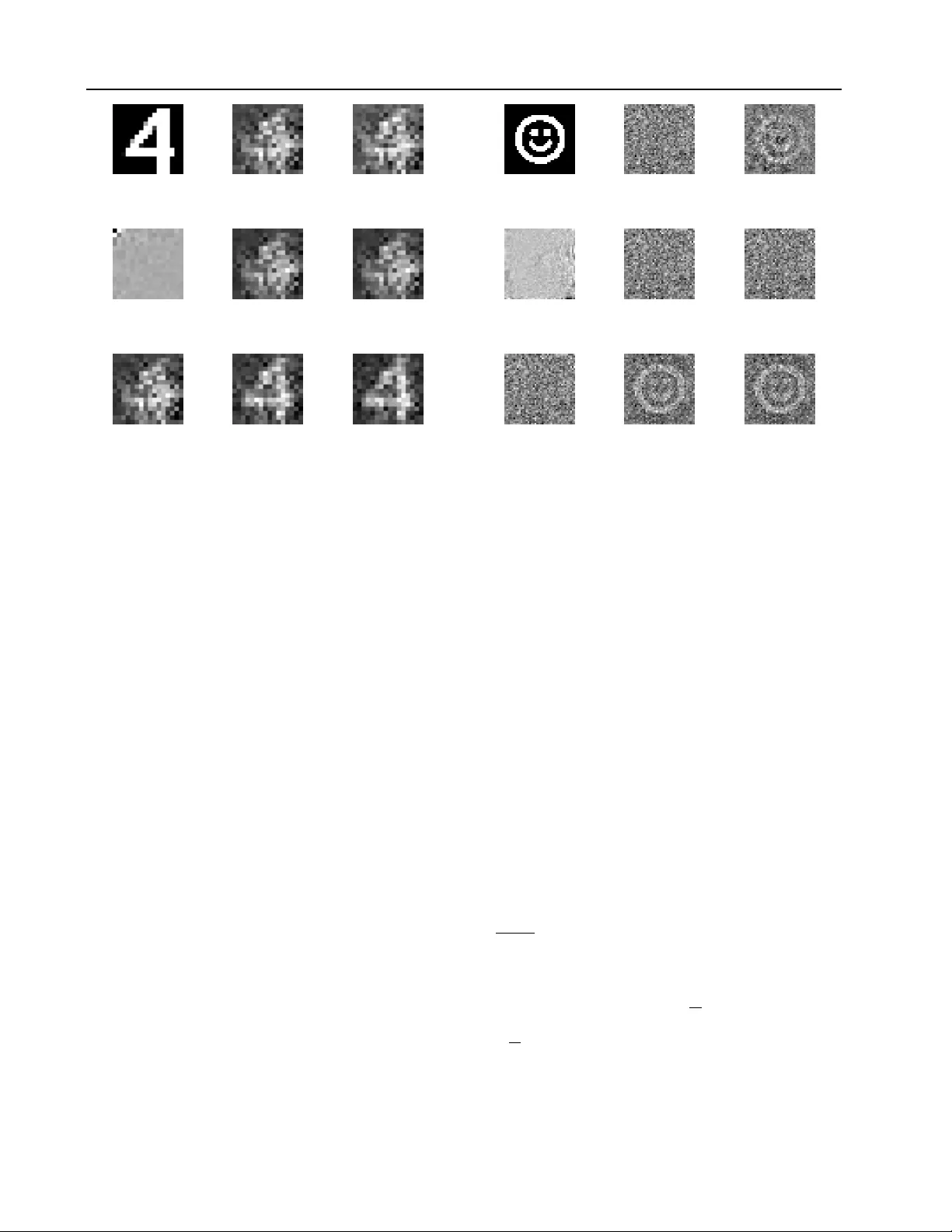
Linear Spectral Estimators and an A pplication to Phase Retriev al Ramina Ghods 1 Andrew S. Lan 2 T om Goldstein 3 Christoph Studer 1 Abstract Phase retrie v al refers to the problem of reco vering real- or complex-v alued vectors from magnitude measurements. The best-known algorithms for this problem are iterativ e in nature and rely on so-called spectral initializers that provide accu- rate initialization vectors. W e propose a nov el class of estimators suitable for general nonlinear measurement systems, called linear spectral esti- mators (LSPEs), which can be used to compute accurate initialization vectors for phase retrie val problems. The proposed LSPEs not only pro vide accurate initialization vectors for noisy phase re- triev al systems with structured or random mea- surement matrices, but also enable the deri v ation of sharp and nonasymptotic mean-squared error bounds. W e demonstrate the ef ficacy of LSPEs on synthetic and real-world phase retrie v al prob- lems, and sho w that our estimators significantly outperform existing methods for structured mea- surement systems that arise in practice. 1. Introduction Phase retrie val refers to the problem of recov ering an un- known N -dimensional signal v ector x ∈ H N , with H being the set of either real ( R ) or complex ( C ) numbers, from the following nonlinear measurement process: y = f ( Ax + e z ) + e y . (1) Here, the measurement vector y ∈ R M contains M real- val ued observations, for example measured through the non- linear function f ( z ) = | z | 2 that operates element-wise on vectors, A ∈ H M × N is a gi ven measurement matrix, and the vectors e z ∈ H M and e y ∈ R N model signal and mea- surement noises, respectiv ely . In contrast to the majority of 1 School of Electrical and Computer Engineering, Cornell Uni- versity , Ithaca, NY 2 Department of EE, Princeton University 3 Univ ersity of Maryland. Correspondence to: Ramina Ghods < rg548@cornell.edu > , Christoph Studer < studer@cornell.edu > . Pr oceedings of the 35 th International Confer ence on Machine Learning , Stockholm, Sweden, PMLR 80, 2018. Cop yright 2018 by the author(s). existing results on phase retrie val that assume randomness in the measurement matrix A , we focus on the practical sce- nario in which the measurement matrix A is deterministic, but the signal vector x to be recovered as well as the two noise sources e z and e y are random. 1.1. Phase Retrieval Phase retriev al has been studied extensi vely ov er the last decades ( Gerchberg & Saxton , 1972 ; Fienup , 1982 ) and finds use in a range of applications, including imaging ( Fo- gel et al. , 2016 ; Y eh et al. , 2015 ; Hollo way et al. , 2016 ), mi- croscopy ( K ou et al. , 2010 ; Faulkner & Rodenb urg , 2004 ), and X-ray crystallography ( Harrison , 1993 ; Miao et al. , 2008 ; Pfeif fer et al. , 2006 ). Phase retriev al problems were solved traditionally using alternating projection methods, such as the Gerchberg-Saxton ( Gerchber g & Saxton , 1972 ) and Fienup ( Fienup , 1982 ) algorithms. More recent results hav e shown that semidefinite programming enables the de- sign of algorithms with performance guarantees ( Cand ` es et al. , 2013 ; Cand ` es & Li , 2014 ; Cand ` es et al. , 2015a ; W ald- spurger et al. , 2015 ). These methods lift the problem to a higher dimension, resulting in e xcessive comple xity and memory requirements. T o perform phase retrie val for high- dimensional problems with performance guarantees, a range of con vex ( Bahmani & Romberg , 2017 ; Goldstein & Studer , 2017 ; Hand & V oroninski , 2016 ; Dhifallah et al. , 2017 ; Dhi- fallah & Lu , 2017 ; Y uan & W ang , 2017 ; Salehi et al. , 2018 ) and noncon vex methods ( Netrapalli et al. , 2013 ; Schniter & Rangan , 2015 ; Cand ` es et al. , 2015b ; Chen & Cand ` es , 2015 ; Zhang & Liang , 2016 ; W ang et al. , 2017a ; Zhang et al. , 2016 ; W ei , 2015 ; Sun et al. , 2016 ; Zeng & So , 2017 ; Lu & Li , 2017 ; Ma et al. , 2018 ) hav e been proposed recently . 1.2. Spectral Initializers All of the abov e non-lifting-based phase retrie val methods rely on accurate initial estimates of the signal vector to be recov ered. Such estimates are typically obtained by means of so-called spectral initializers put forw ard in ( Netrapalli et al. , 2013 ). Spectral initializers first compute a Hermitian matrix of the following form: D β = β M X m =1 T ( y m ) a m a H m , (2) Linear Spectral Estimators and an Application to Phase Retrie val where β > 0 is a suitably-chosen scaling factor , y m denotes the m th measurement, a H m corresponds to the m th row of the measurement matrix A and T : R → R is a (possi- bly nonlinear) prepr ocessing function . While the identity T ( y ) = y was used originally in ( Netrapalli et al. , 2013 ), recent results re vealed that carefully crafted preprocessing functions yield more accurate estimates ( Chen & Cand ` es , 2015 ; Chen et al. , 2015 ; W ang et al. , 2017a ; b ; Lu & Li , 2017 ; Mondelli & Montanari , 2017 ). From the matrix D β in ( 2 ), one then extracts the (scaled) eigen vector ˆ x associ- ated with the lar gest eigen value, which serv es as an initial estimate of the solution to the phase retriev al problem. As shown in ( Netrapalli et al. , 2013 ; Chen & Cand ` es , 2015 ; Chen et al. , 2015 ; W ang et al. , 2017a ; b ; Lu & Li , 2017 ; Mondelli & Montanari , 2017 ), for i.i.d. Gaussian measure- ment matrices A , suf ficiently large measurement ratios δ = M / N , and carefully crafted preprocessing functions T , spectral initializers pro vide accurate initialization vectors. In fact, the results in ( Mondelli & Montanari , 2017 ) for the large-system limit with δ fixed and M → ∞ show that spectral initializers in combination with an optimal prepro- cessing function T achiev e the fundamental information- theoretic limits of phase retriev al. Howe ver , the assump- tion of having i.i.d. Gaussian measurement matrices A is impractical—it is more natural to assume that the signal vector x is random and the measurement matrix A is deter- ministic and structured ( Bendory & Eldar , 2017 ). 1.3. Contributions W e propose a nov el class of estimators, called linear spec- tral estimators (LSPEs) , that pro vide accurate estimates for general nonlinear measurement systems of the form ( 1 ) and enable a nonasymptotic mean-squared error (MSE) analysis. W e sho wcase the efficac y of LSPEs by applying them to phase retrie val problems, where we compute initialization vectors for real- and complex-v alued systems with deter- ministic and finite-dimensional measurement matrices. For the proposed LSPEs, we deri ve nonasymptotic and sharp bounds on the MSE for signal estimation from phaseless measurements. W e use synthetic and real-world phase re- triev al problems to demonstrate that LSPEs are able to sig- nificantly outperform existing spectral initializers on sys- tems that acquire structured measurements. W e furthermore show that preprocessing the phaseless measurements en- ables LSPEs to generate improved initialization v ectors for an ev en broader class of measurement systems. 1.4. Notation Lowercase and uppercase boldface letters represent column vectors and matrices, respecti vely . For a matrix A , its trans- pose and Hermitian conjugate is A T and A H , respectiv ely , and the k th row and ` th column entry is [ A ] k,` = A k,` . For a vector a , the k th entry is [ a ] k = a k . The ` 2 -norm of a is denoted by k a k 2 and the Frobenius norm of A by k A k F . The Kronecker product is ⊗ , the Hadamard product is  , the Hadamard di vision is  , and the trace operator is tr( · ) . The N × N identity matrix is denoted by I N ; the M × N all-zeros and all-ones matrices are denoted by 0 M × N and 1 M × N , respecti vely . For a vector a , diag( a ) is a square ma- trix with a on the main diagonal; for a matrix A , diag( A ) is a column vector containing the diagonal elements of A . 2. Linear Spectral Estimators W e start by revie wing the essentials of spectral initializers and then, introduce linear spectral estimators (LSPEs) for measurement systems of the form ( 1 ) with general nonlinear - ities f . W e furthermore provide nonasymptotic expressions for the associated estimation error , and we compare our analytical results to that of con ventional spectral initializers in ( 2 ). In Section 3 , we will apply LSPEs to phase retrie val. 2.1. Spectral Estimation and Initializers One of the ke y issues of the phase retriev al problem is the fact that if x is a solution to ( 1 ), then e j φ x for any φ ∈ [0 , 2 π ) is also a v alid solution (assuming H = C ). Put simply , the solution is nonunique up to a global phase shift. One way of combating this issue is to directly recov er the outer product xx H instead of x , which is unaffected by phase shifts; this insight is the key underlying lifting-based phase retrie val methods ( Cand ` es et al. , 2013 ; Cand ` es & Li , 2014 ; Cand ` es et al. , 2015a ; W aldspurger et al. , 2015 ). W ith this in mind, one could en vision the design of an estimator that directly minimizes the conditional MSE: ˙ x = arg min ˜ x ∈H N E  k xx H − ˜ x ˜ x H k 2 F | y  . (3) Here, expectation is with respect to the signal v ector x and the two noise sources e z and e y . This optimization problem resembles that of a posterior mean estimator (PME) which is, in general, difficult to deri ve, e ven for simple observ ation models—for phase retriev al, we ha ve two additional chal- lenges: (i) nonlinear phaseless measurements as in ( 1 ) and (ii) the quantity ˜ x ˜ x H has rank-1. Spectral initializers a void the issues of the estimator in ( 3 ) by first replacing the true outer product xx H with a so- called spectral estimator matrix D β as in ( 2 ) that depends on the measurement vector y . In a second step, one then computes the best rank-1 approximation as follows: ˆ x = arg min ˜ x ∈H N k D β − ˜ x ˜ x H k 2 F (4) from which the estimate ˆ x can be extracted. By perform- ing an eigenv alue decomposition D β = UΛU H with U H U = I M and the eigen values in the diagonal matrix Linear Spectral Estimators and an Application to Phase Retrieval Λ = diag([ λ 1 , . . . , λ M ] T ) are sorted in descending order of their magnitudes, a spectral initializer is gi ven by the scaled leading eigen vector ˆ x = √ λ 1 u 1 . In practice, one can use power iterations to ef ficiently compute ˆ x . 2.2. Linear Spectral Estimators W e now propose a no vel class of estimators, which we call linear spectral estimators (LSPEs) , that provide accurate estimates for general nonlinear measurement systems of the form ( 1 ). T o this end, we borrow ideas from the spectral initializer , the PME in ( 3 ), and the linear phase retrie val algorithm put forward in ( Ghods et al. , 2018 ). In the first step, LSPEs apply a linear estimator to the nonlinear obser- vat ions in T ( y ) to construct a spectr al estimator matrix D y for which the spectral MSE (or matrix MSE) defined as S-MSE = E h   D y − xx H   2 F i (5) is minimal. W e restrict ourselves to spectral estimator ma- trices D y that are affine in T ( y ) , i.e., are of the form D y = W 0 + M X m =1 T ( y m ) W m (6) with W m ∈ H N × N , m = 0 , . . . , M . In the second step, we use the spectral estimator matrix D y to e xtract a (scaled) leading eigen vector as in ( 3 ), which is the linear spectral es- timate of the signal v ector x . Intuitively , if we can construct a matrix D y from the preprocessed measurements in T ( y ) for which the S-MSE in ( 5 ) is minimal, then we expect that computing its best rank-1 approximation would yield an accurate estimate of the signal vector x up to a global phase shift. W e will justify this claim in Section 2.3 . Mathematically , we wish to compute a matrix D y of the form ( 6 ) that is the solution to the following problem: minimize f W m ∈H N × N m =0 ,...,M E        f W 0 + M X m =1 T ( y m ) f W m − xx H      2 F   . (7) Clearly , the spectral estimator matrix D y will depend on the measurement matrix A , the statistics of the signal to be estimated x and the two noise sources e z and e y , the nonlinearity f , as well as the preprocessing function T . For this setting, we hav e the following general result which summarizes the LSPE; the proof is giv en in Appendix A . Theorem 1 (Linear Spectral Estimator) . Let the measure- ment vector y be a r esult of the gener al measur ement model in ( 1 ) and select a pr epr ocessing function T . Define the vector T ( y ) = E [ T ( y )] and assume the matrix T = E  ( T ( y ) − T ( y ))( T ( y ) − T ( y )) T  is full rank. Let t ∈ R M satisfy Tt = T ( y ) − T ( y ) and V m = E  ( T ( y m ) − T ( y m ))( xx H − K x )  for m = 1 , . . . , M with K x = E  xx H  . Then, the LSPE matrix that minimizes the S-MSE in ( 5 ) is given by D y = K x + M X m =1 t m V m . (8) The linear spectral estimate ˆ x is then given by the scaled leading eigen vector of the matrix D y in ( 8 ). The vector t is the only quantity in Theorem 1 that depends on the actual (nonlinear) observations contained in the mea- surement vector y . All other quantities depend only on the first two moments of xx H as well as the considered signal, noise, and measurement models. The key features of the LSPE are as follo ws: (i) the in volved quantities can often be computed in closed form (see Section 3 for two applications to phase retriev al) and (ii) LSPEs enable a nonasymptotic and sharp analysis of the associated estimation error . Remark 1. Theor em 1 r equir es the matrix T to be in vert- ible. This condition is satisfied in most practical situations with nonde generate measur ement matrices A or in situa- tions with nonzer o measurement noise . 2.3. Estimation Error Analysis of LSPEs The remaining piece of the proposed LSPE is to sho w that the result of this two-step estimation procedure indeed yields a vector that is close to the signal vector x . W e start with the following result; the proof is gi ven in Appendix B . Theorem 2 (S-MSE of the LSPE) . Let the assumptions of Theor em 1 hold. Then, the S-MSE in ( 5 ) for the LSPE matrix in ( 8 ) is given by S-MSE LSPE = C xx H − M X m =1 M X m 0 =1 [ T − 1 ] m,m 0 tr  V H m V m 0  (9) with C xx H = E h   xx H − K x   2 F i . W ith this result, we are ready to establish a bound on the estimation error of the LSPE. The proof of the following result follows from Theorem 2 and is gi ven in Appendix C . Corollary 1 (LSPE Estimation Error) . Let the assumptions of Theor em 1 hold. Then, the estimation err or (EER) of the LSPE satisfies the following inequality: EER LSPE = E  k ˆ x ˆ x H − xx H k 2 F  ≤ 4 S-MSE LSPE . (10) This result implies that by minimizing the S-MSE in ( 5 ) via ( 7 ), we are also reducing the EER of the LSPE. In other words, if the spectral error E = D y − ˆ x ˆ x H is small, then the EER of the LSPE ( 10 ) will be small. Linear Spectral Estimators and an Application to Phase Retrieval Remark 2. Cor ollary 1 is nonasymptotic and depends on the instance of measur ement matrix A . This r esult is in stark contrast to e xisting performance bounds for spectral initializers ( Netr apalli et al. , 2013 ; Chen & Cand ` es , 2015 ; Chen et al. , 2015 ; W ang et al. , 2017a ; b ) that str ongly rely on randomness in the measur ement matrix. In addition to randomness, the sharp performance guarantees in ( Lu & Li , 2017 ; Mondelli & Montanari , 2017 ) focus on the asymptotic r e gime for which δ = M / N is fixed and M → ∞ . 2.4. S-MSE of Spectral Initializers W e can also derive an exact expression for the S-MSE of the con ventional spectral initializer in ( 2 ). W e assume optimal scaling, i.e., the parameter β is set to minimize the S-MSE. The following result characterizes the S-MSE of such a scaled spectral initializer; the proof is given in Appendix D . Proposition 1 (S-MSE of the Spectral Initializer) . Let D β be the con ventional spectral initializer matrix in ( 2 ). Then, the optimally-scaled S-MSE defined as S-MSE SI = min β ∈H E  k D β − xx H k 2 F  (11) is given by S-MSE SI = R xx H −    P M m =1 a H m e V m a m    2 P M m =1 P M m 0 =1 e T m,m 0 | a H m a m 0 | 2 , (12) wher e R xx H = E  k xx H k 2 F  , e V m = E  T ( y m ) xx H  , m = 1 , . . . , M , and e T = E  T ( y ) T ( y ) T  . Since the matrix in ( 2 ) is a special case of the LSPE matrix in ( 6 ), we have the follo wing simple yet important property: S-MSE LSPE ≤ S-MSE SI . In words, the spectral MSE of the LSPE cannot be worse than that of a spectral initializer . As we will show in Sec- tion 4 , LSPEs are able to outperform spectral initializers on both synthetic and real-world phase retrie val problems giv en that the same preprocessing function T is used. 3. LSPEs for Phase Retrie val Pr oblems The LSPE provides a framew ork for estimating signal vec- tors from the general observation model in ( 1 ). T o make the concept of LSPEs explicit and to demonstrate their ef fi- cacy in practice, we no w show tw o application examples to phase retriev al in complex-valued systems. The LSPE for real-valued phase retrie val can be found in Appendix E . 3.1. Phase Retrieval without Prepr ocessing W e first focus on the case where the signal vector x to be estimated and the measurement matrix A are both complex- valued. The phaseless measurements y , howe ver , remain real-valued. W e need the following assumptions. Assumptions 1. Let H = C . Assume squar e absolute measur ements f ( z ) = | z | 2 and the identity pr eprocessing function T ( y ) = y . Assume that the signal vector x ∈ C N is i.i.d. cir cularly-symmetric complex Gaussian with covari- ance matrix C x = σ 2 x I N , i.e., x ∼ C N ( 0 N × 1 , σ 2 x I N ) . As- sume that the signal noise vector e z is cir cularly-symmetric complex Gaussian with covariance matrix C e z , i.e., e z ∼ C N ( 0 M × 1 , C e z ) , and the measur ement noise vector e y is a r eal-valued Gaussian vector with mean ¯ e y and covariance matrix C e y , i.e ., e y ∼ N ( ¯ e y , C e y ) . Furthermore assume that x , e z , and e y ar e independent. Under these assumptions, we can deri ve the following LSPE which we call LSPE- C ; the detailed deriv ations of this spec- tral estimator are giv en in Appendix G . Estimator 1 (LSPE- C ) . Let Assumptions 1 hold. Then, the spectral estimation matrix is given by D C y = K x + M X m =1 t m V m , (13) wher e K x = σ 2 x I N , the vector t ∈ R M is given by the solution to the linear system Tt = y − y with y = diag( C z ) + ¯ e y C z = σ 2 x AA H + C e z T = C z  C ∗ z + C e y and V m = σ 4 x a m a H m , m = 1 , . . . , M . The spectral esti- mate ˆ x is given by the (scaled) leading eig en vector of D C y in ( 13 ). Furthermore , the S-MSE is given by Theor em 2 . W e emphasize that the spectral estimator matrix in ( 13 ) resembles that of the conv entional spectral initializer ma- trix ( 2 ) with the following ke y differences. First and fore- most, each outer product contained in V m = σ 4 x a m a H m in Estimator 1 is weighted by t m , which is a function of all phaseless measurements in y and of the cov ariance ma- trix C x . In contrast, each outer product in the conv entional spectral initializer matrix in ( 2 ) is only weighted by the asso- ciated measurement y m . This difference enables the LSPE to weight each outer product depending on correlations in the phaseless measurements caused by structure in the ma- trix A . Second, the spectral estimator matrix includes a mean term K x , which is absent in the spectral initializer matrix. As we will show in Section 4 , for the same pre- processing function T , Estimator 1 is able to outperform spectral initializers for systems with structured measurement matrices A . For large i.i.d. Gaussian measurement matrices, there is no particular correlation structure to exploit and LSPEs perform on par with spectral initializers. Linear Spectral Estimators and an Application to Phase Retrieval 3.2. Phase Retrieval with Exponential Prepr ocessing T o demonstrate the flexibility a nd generality of our frame- work, we no w design an LSPE with an exponential prepro- cessing function for complex-valued phase retriev al. W e deriv e the LSPE under the following assumptions. Assumptions 2. Let H = C . Assume square absolute mea- sur ements f ( z ) = | z | 2 and the e xponential prepr ocessing function T ( y ) = exp( − γ y ) with γ > 0 , i.e., we consider T ( y ) = exp  − γ ( | z | 2 + e y )  and z = Ax + e z , wher e the exponential function is applied element-wise to vectors. The r emaining assumptions ar e the same as in Assumptions 1 . W e now deri ve the follo wing LSPE called LSPE-Exp; the deriv ation of this spectral estimator is given in Appendix H . Estimator 2 (LSPE-Exp) . Let Assumptions 2 hold. Then, the spectral estimation matrix is given by D Exp y = K x + M X m =1 t m V m , (14) wher e K x = σ 2 x I N , the vector t ∈ R M is given by the solution to the linear system Tt = T ( y ) − T ( y ) with T ( y ) = p γ  q γ T = ( p γ p T γ )  exp( γ 2 C e y )  ( q γ q T γ − γ 2 C z  C ∗ z ) − ( p γ p T γ )  ( q γ q T γ ) V m = − γ σ 4 x [ p γ ] m ( γ [ C z ] m,m + 1) 2 a m a H m , m = 1 , . . . , M , wher e we use the following definitions: q γ = γ diag( C z ) + 1 M × 1 p γ = exp  − γ ¯ e y + γ 2 1 2 diag( C e y )  C z = σ 2 x AA H + C e z . The spectral estimate ˆ x is given by the (scaled) leading eigen vector of D Exp y in ( 14 ). Furthermor e, the S-MSE of this estimator is given by Theor em 2 . At first sight, the choice of the exponential preprocessing function used in Estimator 2 seems to be arbitrary . W e em- phasize, howe ver , that this particular function is inspired by the asymptotically-optimal preprocessing function for properly-normalized Gaussian measurement ensembles pro- posed in ( Mondelli & Montanari , 2017 ) which is giv en by T opt ( y ) = y − 1 y + √ δ − 1 . (15) As it turns out, we can scale, negate, and shift the e xponen- tial preprocessing function T ( y ) = exp( − γ y ) to make it take a similar shape as the function in ( 15 ). More concretely , exponential preprocessing as well as T opt ( y ) enables one to attenuate the ef fect of measurements with large magnitude, which is also the idea underlying the class of orthogonal spectral initializers, as proposed in ( Chen et al. , 2015 ; W ang et al. , 2017a ; b ), that perform well in practice. 4. Numerical Results W e now compare the performance of our LSPEs against existing spectral initializers proposed for phase retriev al on synthetic and real image data. All our results use the spectral initializers and experimental setups provided by PhasePack ( Chandra et al. , 2017 ). 4.1. Impact of Measurement Ensemble W e start by comparing the normalized MSE (N-MSE) de- fined as ( Chandra et al. , 2017 ) N-MSE = min α ∈H k x − α ˆ x k 2 k x k 2 for a range of spectral initializers on different measurement ensembles. Specifically , we focus on the complex-v alued case and consider (i) an i.i.d. Gaussian measurement ma- trix with signal dimension N = 16 , (ii) an i.i.d. Gaussian measurement matrix with N = 256 , and (iii) the structured “transmission matrix” used for image recovery through mul- tiple scattering media as detailed in ( Metzler et al. , 2017 ). W e vary the ov ersampling ratio δ = M / N and compare the N-MSE of the proposed comple x-valued LSPEs, LSPE- C (Estimator 1 ) and LSPE-Exp (Estimator 2 with γ = 0 . 001 ), to the following spectral initializers: the original spectral ini- tializer ( Netrapalli et al. , 2013 ; Cand ` es et al. , 2015a ) called “spectral, ” truncated spectral initializer ( Chen & Cand ` es , 2015 ) called “truncated, ” weighted spectral initializer ( W ang et al. , 2017b ) called “weighted, ” amplitude spectral initial- izer ( W ang et al. , 2017a ) called “amplitude, ” orthogonal spectral initializer ( Chen et al. , 2015 ) called “orthogonal, ” and the asymptotically-optimal spectral initializer ( Mondelli & Montanari , 2017 ) called “optimal. ” For the follo wing syn- thetic experiments, we generate the signals to be reco vered according to Assumptions 1 and Assumptions 2 for LSPE- C and LSPE-Exp, respectiv ely . Figure 1a shows that the proposed LSPEs significantly out- perform all existing spectral initializers for small problem dimensions with Gaussian measurements; this improv ement is ev en more pronounced for large ov ersampling ratios. The reason is that since we randomly generate a low-dimensional sensing matrix, the system will e xhibit strong correlations among the measurements that can be exploited by LSPEs. For lar ger dimensions with Gaussian measurements, we see in Figure 1b that the proposed LSPEs do not provide an advantage ov er other methods. In fact, only LSPE-Exp is Linear Spectral Estimators and an Application to Phase Retrieval 0 2 4 6 8 10 12 14 16 10 − 3 10 − 2 10 − 1 10 0 10 1 oversampling ratio: δ = M / N normalized MSE: N-MSE spectral truncated amplitude weighted optimal orthogonal LSPE- C LSPE-Exp (a) Gaussian measur ements, N = 16 . 0 10 20 30 40 50 60 70 10 − 3 10 − 2 10 − 1 10 0 10 1 oversampling ratio: δ = M / N normalized MSE: N-MSE spectral truncated amplitude weighted optimal orthogonal LSPE- C LSPE-Exp (b) Gaussian measur ements, N = 256 . 0 10 20 30 40 50 60 70 10 − 3 10 − 2 10 − 1 10 0 10 1 oversampling ratio: δ = M / N normalized MSE: N-MSE spectral truncated amplitude weighted optimal orthogonal LSPE- C LSPE-Exp (c) T ransmission measur ements, N = 256 . Figure 1: Comparison of normalized MSE (N-MSE) as a function of the oversampling ratio δ = M / N for complex-valued phase r etrieval with differ ent spectral initializers and with differ ent measur ement matrices. The pr oposed LSPEs perform well on low-dimensional pr oblems, for structured measur ement ensembles, or at high oversampling r atios δ . able to perform as well as the orthogonal spectral initial- izer , which achiev es the best performance in this scenario. This behavior can be attrib uted to the facts that (i) for large random matrices there is no particular correlation structure among the measurements to e xploit and (ii) ignoring mea- surements associated to large values in y m is increasingly important. For structured measurements, as it is the case for the transmission matrix from ( Metzler et al. , 2017 ), we see in Figure 1c that LSPEs significantly outperform e xisting methods that are designed for random measurement ensem- bles. In this scenario, e xponential preprocessing does not improv e performance since correlations in the transmission matrix are dominating the performance. 4.2. S-MSE Expressions and Appr oximation Error W e now v alidate our theoretical S-MSE expressions in The- orem 2 and Proposition 1 , and confirm the accurac y of the EER bound gi ven in Corollary 1 . In the following exper - iment, we set M = 8 N and vary the dimension N from 8 to 64 . For each pair ( M , N ) , we randomly generate one instance of an i.i.d. circularly symmetric complex Gaus- sian measurement matrix and av erage the dif ferent errors (S-MSE and EER) over 10 , 000 Monte-Carlo trials. W e con- sider a noiseless setting and assume identity preprocessing, i.e., T ( y ) = y . The signal vectors are generated accord- ing to an i.i.d. circularly complex Gaussian random vector . From Figure 2 , we see that our analytical S-MSE expres- sions for the LSPE- C and spectral initializers match their empirical values. W e furthermore see that the empirical EER is only about 6 dB to 10 dB lo wer than our non-asymptotic upper bound giv en in Corollary 1 . 4.3. Real-W orld Image Recovery W e finally illustrate the efficacy of LSPEs in a more realistic scenario. In particular , we show results for a real image reconstruction task by using LSPEs and spectral initializers 0 10 20 30 40 50 60 70 0 10 20 30 40 50 signal dimension N S-MSE or EER in [dB] S-MSE LSPE , empirical S-MSE LSPE , analytical (9) S-MSE SI , empirical S-MSE SI , analytical (12) EER LSPE , empirical EER LSPE , upper bound (1) Figure 2: Comparison of the analytical and empirical spec- tral MSE (S-MSE) and estimation err or (EER) for LSPEs and spectr al initializers (SI) at oversampling ratio δ = 8 . Our analytical expr essions in Theorem 2 and Pr oposition 1 match the empirical S-MSE; the upper bound in Cor ollary 1 accurately c haracterizes the empirical EER. only , i.e., we are not using an y additional phase retriev al al- gorithm. Our goal is to recover a 16 × 16 -pixel and a 40 × 40 - pixel image that was captured through a multiple scattering media using the deterministic and highly-structured trans- mission matrix as detailed in ( Metzler et al. , 2017 ). W e compare the proposed LSPEs to the same set of spectral initializers as in Section 4.1 . The signal priors are as in Assumptions 1 (LSPE- C ) and Assumptions 2 (LSPE-Exp). Figures 3 and 4 sho w the recovered images along with the N-MSE values. The proposed LSPEs (often significantly) outperform all spectral initializers in terms of visual quality as well as the N-MSE. This result confirms the observ ations made in Figure 1c that LSPEs outperform existing spec- tral initializers for structured measurement matrices. W e note that exponential preprocessing for LSPEs does not no- ticeably improv e the N-MSE (ov er LSPE- C ) in this setting since correlations in the transmission measurement matrix are dominating the recov ery performance. Linear Spectral Estimators and an Application to Phase Retrieval (a) original (b) amplitude N-MSE = 0 . 4927 (c) optimal N-MSE = 0 . 4833 (d) orthogonal N-MSE = 0 . 6850 (e) spectral N-MSE = 0 . 4764 (f) truncated N-MSE = 0 . 4764 (g) weighted N-MSE = 0 . 4797 (h) LSPE- C N-MSE = 0 . 3377 (i) LSPE-Exp N-MSE = 0 . 2928 Figure 3: Recovery of a 16 × 16 image fr om with M = 5 N measur ements captur ed through a scattering medium with- out the use of a phase r etrieval algorithm. LSPEs outper - form all initializers for structur ed measurements. 5. Conclusions W e hav e proposed a novel class of estimators, called lin- ear spectral estimators (LSPEs), which are suitable for the recov ery of signals from general nonlinear measurement systems. W e have de veloped nonasymptotic and determinis- tic performance guarantees for LSPEs that pro vide accurate bounds on the estimation error , especially for structured or low-dimensional measurement systems. T o demonstrate the ef ficacy of LSPEs in practice, we ha ve applied them to complex-v alued phase retriev al problems, in which LSPEs can be used to compute accurate signal estimates or ini- tialization vectors for other con vex or noncon vex phase retriev al algorithms. W e have sho wn that properly prepro- cessing the nonlinear measurements can further improv e the performance of LSPEs in practical scenarios. Our simula- tions with synthetic and real data have shown that LSPEs are able to significantly outperform existing spectral initializ- ers, especially for low-dimensional problems, for structured measurement matrices, or for large o versampling ratios. There are man y a venues for future work. First, one could deriv e LSPEs for the asymptotically-optimal preprocess- ing function in ( 15 ) or for other commonly used functions, which may lead to further performance improvements. Sec- ond, the proposed error analysis could be used to generate improv ed measurement matrices. Third, an exploration of LSPEs for other nonlinearities that arise in machine learning and signal processing applications is left for future work. (a) original (b) amplitude N-MSE = 0 . 7010 (c) optimal N-MSE = 0 . 5849 (d) orthogonal N-MSE = 0 . 7028 (e) spectral N-MSE = 0 . 7016 (f) truncated N-MSE = 0 . 7020 (g) weighted N-MSE = 0 . 7013 (h) LSPE- C N-MSE = 0 . 4920 (i) LSPE-Exp N-MSE = 0 . 4896 Figure 4: Reco very of a 40 × 40 image fr om with M = 10 N measur ements captur ed through a scattering medium with- out the use of a phase r etrieval algorithm. LSPEs outper - form all initializers for structur ed measurements. Acknowledgments R. Ghods and C. Studer were supported in part by Xilinx, Inc. and by the US National Science Foundation (NSF) un- der grants ECCS-1408006, EECS-1740286, CCF-1535897, CCF-1652065, and CNS-1717559. T . Goldstein was sup- ported by the US NSF under grant CCF-1535902, the US ONR under grant N00014-15-1-2676, the D ARP A Lifelong Learning Machines program, and the Sloan Foundation. A. Proof of Theor em 1 The proof proceeds in two steps detailed as follo ws. Mean Matrix W e first compute the mean matrix W 0 . Since ( 7 ) is a quadratic form, we can take the deriv ative in f W H 0 and set it to zero, i.e., d d f W H 0 E        f W 0 + M X m =1 T ( y m ) f W m − xx H      2 F   = 0 . Basic matrix calculus yields f W 0 = K x − P M m =1 T ( y m ) f W m (16) with T ( y m ) = E [ T ( y m )] and K x = E  xx H  . Linear Estimation Matrix W ith ( 16 ) and the fact that ( 7 ) is a quadratic form in the matrices W m , m = 1 , . . . , M , Linear Spectral Estimators and an Application to Phase Retrieval we take the deri vati ves in W H m and setting them to zero: d d f W H m E "     M X m =1 ( T ( y m ) − T ( y m )) f W m − ( xx H − K x )     2 F # = 0 . By interchanging the deri vati ve with expectation and with basic manipulations, we obtain the following set of optimal- ity conditions for W m for m = 1 , . . . , M : P M m 0 =1 f W m 0 E  ( T ( y m ) − T ( y m ))( T ( y m 0 ) − T ( y m 0 ))  = E  ( T ( y m ) − T ( y m ))( xx H − K x )  . (17) In compact matrix form, the abov e condition reads ( T ⊗ I N × N ) W = V , (18) where we used the following shortcuts: T = E  ( T ( y ) − T ( y ))( T ( y ) − T ( y )) T  W = [ f W T 1 , . . . , f W T m , . . . , f W T M ] T V m = E  ( T ( y m ) − T ( y m ))( xx H − K x )  , m = 1 , . . . , M V = [ V T 1 , . . . , V T m , . . . , V T M ] T . The condition in ( 18 ) can be solved for the estimation ma- trices in W leading to W = ( T − 1 ⊗ I N × N ) V , where we require the matrix T to be full rank. T o obtain the linear spectral estimator matrix, we simplify as D y = K x + (( T ( y ) − T ( y )) T ⊗ I N × N ) W = K x + P M m =1 t m V m , where we define the vector t = T − 1 ( T ( y ) − T ( y )) . B. Proof of Theor em 2 T o compute the spectral MSE in ( 5 ), we simplify S-MSE = E     P M m =1 t m V m − ( xx H − K x )    2 F  . W e expand this expression into four terms E     P M m =1 t m V m − ( xx H − K x )    2 F  = E     P M m =1 t m V m    2 F  (19) + E h   xx H − K x   2 F i − E h tr  ( xx H − K x ) H  P M m =1 t m V m i (20) − E  tr   P M m =1 t m V m  H ( xx H − K x )  (21) and simplify each expression indi vidually . W e start with ( 19 ) and use the fact that P M m =1 t m V m = (( T ( y ) − T ( y )) T T − 1 ⊗ I N × N ) V and rewrite the quantity within e xpectation as follows: V H ( T − 1 ( T ( y ) − T ( y )) ⊗ I N × N ) × (( T ( y ) − T ( y )) T T − 1 ⊗ I N × N ) V = V H (( T − 1 ( T ( y ) − T ( y )) × ( T ( y ) − T ( y )) T T − 1 ) ⊗ I N × N ) V . W e now e valuate the expectation which leads to E     P M m =1 t m V m    2 F  = tr  V H ( T − 1 ⊗ I N × N ) V  or , equiv alently , to E     P M m =1 t m V m    2 F  = M X m =1 M X m 0 =1 [ T − 1 ] m,m 0 tr  V H m V m 0  . W e next will simplify ( 20 ). Recall that t m = P M m 0 =1 [ T − 1 ] m,m 0 ( T ( y m 0 ) − T ( y m 0 )) , which enables us to write ( 20 ) as E h tr  ( xx H − K x ) H  P M m =1 t m V m i = P M m =1 P M m 0 =1 [ T − 1 ] m,m 0 × tr  E  ( xx H − K x ) H ( T ( y m 0 ) − T ( y m 0 ))  V m  = P M m =1 P M m 0 =1 [ T − 1 ] m,m 0 tr  V H m 0 V m  . (22) Seeing as ( 21 ) is the Hermitian conjugate of ( 20 ), we hav e E  tr   P M m =1 t m V m  H ( xx H − K x )  = P M m =1 P M m 0 =1 [ T − 1 ] ∗ m,m 0 tr  V H m V m 0  . (23) Combining all these terms yield the spectral MSE S-MSE = E     P M m =1 t m V m − ( xx H − K x )    2 F  = C xx H − tr  V H ( T − 1 ⊗ I N × N ) V  . with C xx H = E h   xx H − K x   2 F i . C. Proof of Cor ollary 1 W e bound the estimation error with the spectral MSE of the LSPE as follows. F or a giv en instance, we hav e k ˆ x ˆ x H − xx H k 2 F = k ˆ x ˆ x H − D y + D y − xx H k 2 F (a) ≤ 2 k ˆ x ˆ x H − D y k 2 F + 2 k D y − xx H k 2 F (b) ≤ 4 k D y − xx H k 2 F , where (a) follo ws from the squared triangle inequality and (b) because ˆ x ˆ x H is the best rank-1 approximation of D y . A veraging ov er all instances finally yields E  k ˆ x ˆ x H − xx H k 2 F  ≤ 4 S-MSE LSPE . Linear Spectral Estimators and an Application to Phase Retrieval D. Pr oof of Proposition 1 Our goal is to first ev aluate the S-MSE of the unnormalized spectral initializer in ( 2 ) US-MSE SI = E        β M X m =1 T ( y m ) a m a H m − xx H      2 F   and then minimize the resulting expression o ver the param- eter β . The unnormalized spectral MSE can be e xpanded into the following form: | β | 2 M X m =1 M X m 0 =1 E [ T ( y m ) T ( y m 0 )] tr( a m a H m a m 0 a H m 0 ) − β ∗ M X m =1 tr  a m a H m E  T ( y m ) xx H  − β M X m =1 tr  E  xx H T ( y m )  a m a H m  + E  k xx H k 2 F  . By using the definitions e V m = E  T ( y m ) xx H  , m = 1 , . . . , M , e T = E  T ( y ) T ( y ) T  , we can simplify the abov e expression into | β | 2 M X m =1 M X m 0 =1 e T m,m 0 | a H m a m 0 | 2 + E  k xx H k 2 F  − β ∗ M X m =1 tr  a m a H m e V m  − β M X m =1 tr  e V H m a m a H m  . (24) W e can now find the optimal parameter for β by taking the deriv ative with respect to β ∗ and setting the expression to zero. The resulting optimal scaling parameter is giv en by ˆ β = P M m =1 tr  a m a H m e V m  P M m =1 P M m 0 =1 e T m,m 0 | a H m a m 0 | 2 . W e now plug in ˆ β into the expression ( 24 ), which yields S-MSE SI =       P M m =1 tr  a m a H m e V m  P M m =1 P M m 0 =1 e T m,m 0 | a H m a m 0 | 2       2 (25) × M X m =1 M X m 0 =1 e T m,m 0 | a H m a m 0 | 2 − P M m =1 tr  e V H m a m a H m  P M m =1 P M m 0 =1 e T ∗ m,m 0 | a H m a m 0 | 2 M X m =1 tr  a m a H m e V m  − P M m =1 tr  a m a H m e V m  P M m =1 P M m 0 =1 e T m,m 0 | a H m a m 0 | 2 M X m =1 tr  e V H m a m a H m  + E  k xx H k 2 F  . This expression can be simplified further to obtain: S-MSE SI =    P M m =1 tr  a m a H m e V m     2 P M m =1 P M m 0 =1 e T ∗ m,m 0 | a H m a m 0 | 2 −    P M m =1 tr  a m a H m e V m     2 P M m =1 P M m 0 =1 e T ∗ m,m 0 | a H m a m 0 | 2 −    P M m =1 tr  a m a H m e V m     2 P M m =1 P M m 0 =1 e T m,m 0 | a H m a m 0 | 2 + E  k xx H k 2 F  , = R xx H −    P M m =1 a H m e V m a m    2 P M m =1 P M m 0 =1 e T m,m 0 | a H m a m 0 | 2 , which is what we wanted to sho w in ( 12 ). E. Real-V alued Phase Retriev al W e no w focus on the case where the signal v ector x to be re- cov ered and the measurement matrix A are both real-valued. W e derive the LSPE by using the following assumptions, which are reasonable for phase retriev al problems. Assumptions 3. Let H = R . Assume square measur e- ments f ( z ) = z 2 and the identity prepr ocessing function T ( y ) = y . Assume that the signal vector x ∈ R N is i.i.d. zer o-mean Gaussian distributed with covariance matrix C x = σ 2 x I N , i.e., x ∼ N ( 0 N × 1 , σ 2 x I N ) ; the parameter σ 2 x denotes the signal variance . Assume that the signal noise vector e z is zer o-mean Gaussian with covariance matrix C e z , i.e., e z ∼ N ( 0 M × 1 , C e z ) , and the measur ement noise vector e y is Gaussian with mean ¯ e y and covariance matrix C e y , i.e., e y ∼ N ( ¯ e y , C e y ) . Furthermor e assume that x , e z , and e y ar e independent. Under these assumptions, we can deri ve the following LSPE which we call LSPE- R ; the detailed deriv ations of this spec- tral estimator are giv en in Appendix F . Estimator 3 (LSPE- R ) . Let Assumptions 3 hold. Then, the spectral estimation matrix is given by D R y = K x + M X m =1 t m V m , (26) wher e K x = σ 2 x I N , the vector t ∈ R M is given by the solution to the linear system Tt = y − y with y = diag( C z ) + ¯ e y Linear Spectral Estimators and an Application to Phase Retrieval C z = σ 2 x AA T + C e z T = 2 C z  C z + C e y and V m = 2 σ 4 x a m a T m , m = 1 , . . . , M . The spectral esti- mate ˆ x is given by the (scaled) leading eig en vector of D R y in ( 26 ). Furthermore , the S-MSE is given by Theor em 2 . F . Derivation of Estimator 3 W e no w use Theorem 1 to deri ve Estimator 3 under Assump- tions 3 . T o this end, we require the three quantities: T ( y ) , T , and V m , m = 1 , . . . , M , which we deriv e separately . Computing T ( y ) T o compute the real-valued v ector T ( y ) = E [ T ( y )] , (27) we need the following result on the bi variate folded normal distribution de veloped in ( Kan & Robotti , 2017 , Sec. 3.1). Lemma 1. Let [ u 1 , u 2 ] ∼ N ( µ , Σ ) be a pair of real-valued jointly Gaussian random variables with covariance matrix Σ =  σ 2 1 σ 2 1 , 2 σ 2 1 , 2 σ 2 2  . Then, for m = 1 , 2 , the pair of random variables ( ν 1 , ν 2 ) with ν 1 = u 2 1 and ν 2 = u 2 2 follows the bivariate folded normal distribution with the following (center ed) moments: ¯ ν m = E  u 2 m  = σ 2 m + µ 2 m [ C ν ] 1 , 2 = E [( ν 1 − ¯ ν 1 )( ν 2 − ¯ ν 2 )] = 4 µ 1 µ 2 σ 2 1 , 2 + 2 σ 4 1 , 2 [ C ν ] 1 , 1 = E  ( ν 1 − ¯ ν 1 ) 2  = 2 σ 4 1 + 4 µ 2 1 σ 2 1 . Let ¯ z = E [ z ] denote the mean v ector and C z = A C x A H + C e z = σ 2 x AA H + C e z the cov ariance matrix of the “phased” measurements z = Ax + e z . Then, by defin- ing σ 2 m = [ C z ] m,m , we can compute the m th entry T ( y m ) using Lemma 1 as follows: T ( y m ) = ¯ y m = E  | z m | 2 + n y m  = σ 2 m + ¯ e y m . (28) Hence, in compact vector notation we ha ve T ( y ) = ¯ y = diag( C z ) + ¯ e y . (29) Computing T T o compute the real-valued matrix T = E  ( T ( y ) − T ( y ))( T ( y ) − T ( y )) T  = E  T ( y ) T ( y ) T  − T ( y ) T ( y ) T , (30) we only need to compute the matrix E  T ( y ) T ( y ) T  as the vector T ( y ) was computed in ( 29 ). W e compute this matrix entry-wise as T m,m 0 = E  ( T ( y m ) − T ( y m ))( T ( y m 0 ) − T ( y m 0 ))  = E [ y m y ∗ m 0 ] − ¯ y m ¯ y ∗ m 0 (a) = E  ( | z m | 2 + e y m )( | z m 0 | 2 + e y m 0 )  − ( σ 2 m + ¯ e y m )( σ 2 m 0 + ¯ e y m 0 ) = E  | z m | 2 | z m 0 | 2  − σ 2 m 0 σ 2 m + [ C e y ] m,m 0 , where (a) follows from ( 28 ). The only unknown term in the above e xpression is E  | z m | 2 | z m 0 | 2  . This term is the second moment of the random vector [ | z m | 2 , | z m 0 | 2 ] , which follows a bi variate folded normal distribution. For m 6 = m 0 , Lemma 1 yields E  | z m | 2 | z m 0 | 2  = σ 2 m σ 2 m 0 + 2 σ 4 m,m 0 with σ 2 m,m 0 = [ C z ] m,m 0 . For m = m 0 , Lemma 1 yields E  | y m | 2  = E  | z m | 4  = 3 σ 4 m . Hence, we hav e T m,m 0 = [ C e y ] m,m 0 +  2 σ 4 m,m 0 if m 6 = m 0 2 σ 4 m if m = m 0 , which can be written in compact matrix form as T = 2 C z  C z + C e y . Computing V m T o compute the matrices V m = E  ( T ( y m ) − T ( y m ))( xx H − K x )  = E  T ( y m ) xx H  − T ( y m ) K x (31) for m = 1 , . . . , M , we only need to compute the comple x- valued matrix E  T ( y m ) xx H  as the two other quantities K x = E  xx H  and T ( y m ) are kno wn. W e compute this matrix entry-wise as [ V m ] n,n 0 = E  ( T ( y m ) − T ( y m )) x n x ∗ n 0  = E [ y m x n x ∗ n 0 ] − ¯ y m [ C x ] n,n 0 . Since ¯ y m is known from ( 28 ), we focus on computing E [ y m x n x ∗ n 0 ] = E "  N X j =1 A ∗ m,j x ∗ j + e z m  ×  N X j 0 =1 A m,j 0 x j 0 + e z m  + e y m ! x n x ∗ n 0 # = E "  N X j =1 A ∗ m,j x ∗ j N X j 0 =1 A m,j 0 x j 0  x n x ∗ n 0 # + E  | e z m | 2 x n x ∗ n 0  + E [ e y m x n x ∗ n 0 ] = N X j =1 A ∗ m,j N X j 0 =1 A m,j 0 E  x ∗ j x j 0 x n x ∗ n 0  (32) Linear Spectral Estimators and an Application to Phase Retrieval + ([ C e z ] m,m + ¯ e y m )[ C x ] n,n 0 . The only unknown in the above expression is the double summation in ( 32 ). Since we assumed that the entries of the signal vector x are i.i.d., most of the terms in this summation are zero. For n 6 = n 0 , there are only two nonzero terms, corresponding to the cases of ( j, j 0 ) = ( n, n 0 ) and ( j, j 0 ) = ( n 0 , n ) . Thus, for n 6 = n 0 we hav e N X j =1 A ∗ m,j N X j 0 =1 A m,j 0 E  x ∗ j x j 0 x n x ∗ n 0  = 2 A ∗ m,n A m,n 0 E  | x n | 2 | x n 0 | 2  (b) = 2 A ∗ m,n A m,n 0 [ C x ] n,n [ C x ] n 0 ,n 0 , (33) where (b) follows from Lemma 1 . F or n = n 0 , we hav e N X j =1 A ∗ m,j N X j 0 =1 A m,j 0 E  x ∗ j x j 0 x n x ∗ n  = | A m,n | 2 E  | x n | 4  + N X j 6 = n,j =1 | A m,j | 2 E  | x j | 2 | x n | 2  (c) = 3 | A m,n | 2 [ C x ] 2 n,n + N X j 6 = n,j =1 | A m,j | 2 [ C x ] j,j [ C x ] n,n = 2 | A m,n | 2 [ C x ] 2 n,n + N X j =1 | A m,j | 2 [ C x ] j,j [ C x ] n,n . As for ( 33 ), (c) follo ws from Lemma 1 . By combining the abov e results, we hav e V m = 2 C H x a m a H m C x + ( a H m C x a m )( C H x  I ) + ([ C e z ] m,m − σ 2 m ) C x = 2 σ 4 x a m a H m , where a H m denotes the m th row of the matrix A . G. Derivation of Estimator 1 W e no w use Theorem 1 to deri ve Estimator 1 under Assump- tions 1 . T o this end, we require the three quantities: T ( y ) , T , and V m , m = 1 , . . . , M , which we deriv e separately . Computing T ( y ) T o compute the real-v alued vector T ( y ) = ¯ y in ( 27 ), we need the follo wing definitions. Let ¯ z = E [ z ] denote the mean vector and C z = A C x A H + C e z = σ 2 x AA H + C e z the cov ariance matrix of the “phased” measurements z = Ax + e z . Then, using Lemma 1 with the definitions ¯ z and C z , we hav e ¯ y m = E  | z m | 2 + ¯ e y m  = E  | z m, R | 2 + | z m, I | 2 + ¯ e y m  = σ 2 m + ¯ e y m , (34) where we ha ve used the definition σ 2 m = [ C z ] m,m . Hence, in compact vector notation we ha ve T ( y ) = ¯ y = diag( C z ) + ¯ e y . Computing T T o compute the real-v alued matrix T in ( 30 ), we will frequently use the followi ng result. Since the vector z is a complex circularly-symmetric jointly Gaus- sian v ector , we can extract the cov ariance matrices of the real and imaginary parts separately as: E  z I z H I  (a) = E  z R z H R  = 1 2 <{ C z } = 1 2 C z , R (35) E  z R z H I  = − E  z I z H R  = 1 2 ={ C z } = 1 2 C z , I , (36) where (a) follows from circular symmetry of the random vector x . W e are now ready to compute the individual entries of E  T ( y ) T ( y ) T  as T m,m 0 = E  ( T ( y m ) − T ( y m ))( T ( y m 0 ) − T ( y m 0 ))  = E [( y m − ¯ y m )( y m 0 − ¯ y m 0 ) ∗ ] = E [ y m y ∗ m 0 ] − ¯ y m ¯ y ∗ m 0 . The quantity ¯ y m is giv en by ( 34 ). Hence, we now compute E [ y m y ∗ m 0 ] = E  ( | z m | 2 + e y m )( | z 0 m | 2 + e y m 0 ) ∗  = E  | z m, R | 2 + | z m, I | 2   | z m 0 , R | 2 + | z m 0 , I | 2  + [ C e y ] m,m = 2 E  | z m, R | 2 | z m 0 , R | 2  + 2 E  | z m, R | 2 | z m 0 , I | 2  + [ C e y ] m,m . The first two terms abo ve are a second moment of the v ari- ables [ | z m, R | 2 , | z m 0 , R | 2 ] and [ | z m, R | 2 , | z m 0 , I | 2 ] , which fol- low a biv ariate folded normal distributions. W e first fo- cus on [ | z m, R | 2 , | z m 0 , R | 2 ] . W ith Lemma 1 , we can cal- culate the moments using the covariance E  z R z H R  giv en in ( 35 ). T o this end, define σ 2 m,m 0 , R = [ C z , R ] m,m 0 and σ 2 m, R = [ C z , R ] m,m . Thus, we have E  | z m, R | 2 | z m 0 , R | 2  = ( σ 2 m, R 2 σ 2 m 0 , R 2 + σ 4 m,m 0 , R 2 , m 6 = m 0 3 σ 4 m, R 4 , m = m 0 . Analogously , we can compute E  z R z H I  in ( 36 ) from the cov ariance matrix of [ | z m, R | 2 , | z m 0 , I | 2 ] , with σ 2 m,m 0 , I = [ C z , I ] m,m 0 and noting that σ 2 m, I = [ C z , I ] m,m = 0 as E  | z m, R | 2 | z m 0 , I | 2  = ( σ 2 m, R 2 σ 2 m 0 , R 2 + 2 σ 4 m,m 0 , I 4 , m 6 = m 0 3 σ 4 m, R 4 , m = m 0 . By combining the abov e results, we hav e T m,m 0 =  σ 2 m, R σ 2 m 0 , R + σ 4 m,m 0 , R + σ 4 m,m 0 , I , m 6 = m 0 2 σ 4 m, R , m = m 0 , + [ C e y ] m,m 0 − ¯ y m ¯ y ∗ m 0 = [ C e y ] m,m 0 +  σ 4 m,m 0 , R + σ 4 m,m 0 , I , m 6 = m 0 σ 4 m, R , m = m 0 , which can be written in matrix form as T = C z  C ∗ z + C e y . Linear Spectral Estimators and an Application to Phase Retrieval Computing V m T o compute the matrices V m , m = 1 , . . . , M , in ( 31 ), we need the complex-v alued matrix E  T ( y m ) xx H  . W e compute this matrix entry-wise as [ V m ] n,n 0 = E  ( T ( y m ) − T ( y m )) x n x ∗ n 0  = E [ y m x n x ∗ n 0 ] − ¯ y m [ C x ] n,n 0 . Since ¯ y m is giv en by ( 34 ), we only need to compute E [ y m x n x ∗ n 0 ] = E "   N X j =1 A ∗ m,j x ∗ j + e z ∗ m  ×  N X j 0 =1 A m,j 0 x j 0 + e z m  + e y m  x n x ∗ n 0 # = N X j =1 A ∗ m,j N X j 0 =1 A m,j 0 E  x ∗ j x j 0 x n x ∗ n 0  + E  | e z m | 2 x n x ∗ n 0  + E [ e y m x n x ∗ n 0 ] = N X j =1 A ∗ m,j N X j 0 =1 A m,j 0 E  x ∗ j x j 0 x n x ∗ n 0  (37) + ([ C e z ] m,m + ¯ e y m )[ C x ] n,n 0 . W e will first simplify the term N X j =1 A ∗ m,j N X j 0 =1 A m,j 0 E  x ∗ j x j 0 x n x ∗ n 0  . Since we assumed that the signal vector x has i.i.d. zero- mean entries, most of the terms in this summation are zero. For n 6 = n 0 , there is only one non-zero term for ( j, j 0 ) = ( n, n 0 ) . Thus, for n 6 = n 0 we hav e N X j =1 A ∗ m,j N X j 0 =1 A m,j 0 E  x ∗ j x j 0 x n x ∗ n 0  = A ∗ m,n A m,n 0 [ C x ] n,n [ C x ] n 0 ,n 0 , since the term that corresponds to ( j, j 0 ) = ( n 0 , n ) , i.e. A ∗ m,n 0 A m,n E [ x ∗ n 0 x ∗ n 0 ] E [ x n x n ] , is zero. Next, for n = n 0 , we hav e N X j =1 A ∗ m,j N X j 0 =1 A m,j 0 E  x ∗ j x j 0 x n x ∗ n 0  = | A m,n | 2 E  | x n | 4  + N X j 6 = k,j =1 | A m,j | 2 E  | x j | 2 | x n | 2  = | A m,n | 2 E  | x n, R | 4  + | A m,n | 2 E  | x n, I | 4  + 2 | A m,n | 2 E  | x n, R | 2 | x n, I | 2  + N X j 6 = n,j =1 | A m,j | 2 × E  ( | x j, R | 2 + | x j, I | 2 )( | x n, R | 2 + | x n, I | 2 )  (a) = 2 | A m,n | 2 E  | x n, R | 4  + 2 N X j =1 | A m,j | 2 E  | x j, R | 2 | x n, I | 2  + 2 N X j 6 = n,j =1 | A m,j | 2 E  | x j, R | 2 | x n, R | 2  (b) = | A m,n | 2 [ C x ] 2 n,n + N X j =1 | A m,j | 2 [ C x ] j,j [ C x ] n,n , where (a) follo ws from circular symmetry of x and (b) from Lemma 1 . By combining the above results, we ha ve V m = C H x a m a H m C x + ( a H m C x a m )( C H x  I ) + ([ C e z ] m,m − σ 2 m ) C x = σ 4 x a m a H m . H. Derivation of Estimator 2 W e no w use Theorem 1 to deri ve Estimator 2 under Assump- tions 2 . T o this end, we require the three quantities: T ( y ) , T , and V m , m = 1 , . . . , M , which we deriv e separately . Computing T ( y ) T o derive an expression for T ( y ) in ( 27 ), we need the following tw o results. Lemma 2. Let u ∼ C N ( 0 M × 1 , Σ ) be a complex-valued cir cularly-symmetric jointly Gaussian r andom vector with positive definite covariance matrix Σ ∈ C M × M . Then, for the random variable ν = exp( − u H Gu ) with positive definite G ∈ C M × M and G + Σ − 1 positive definite, we have the following r esult: E [ ν ] = 1 | G Σ + I M | . Pr oof. W e first expand the expected v alue into E [ ν ] = E  exp( − u H Gu )  = Z C M exp( − u H Gu ) 1 π M | Σ | exp( − u H Σ − 1 u ) d u , where | Σ | > 0 is the determinant of Σ . W e can no w simplify the abov e expression as follo ws: Z C M exp( − u H Gu ) 1 π M | Σ | exp( − u H Σ − 1 u ) d u = Z C M 1 π M | Σ | exp  − u H ( G + Σ − 1 ) u  d u = π M | ( G + Σ − 1 ) − 1 | π M | Σ | 1 π M | ( G + Σ − 1 ) − 1 | × Z C M exp  − u H ( G + Σ − 1 ) u  d u Linear Spectral Estimators and an Application to Phase Retrieval = | ( G + Σ − 1 ) − 1 | | Σ | = 1 | G + Σ − 1 || Σ | = 1 | G Σ + I | , where we also required that G + Σ − 1 is positiv e definite.  Lemma 3. Let u ∼ N ( ¯ u , Σ ) be a r eal-valued Gaussian random vector with mean ¯ u and co variance Σ , and γ ∈ R N be a given vector . Then, we have E  exp( − γ T u )  = exp  − γ T ¯ u + 1 2 γ T Σ γ  . Pr oof. The proof is an immediate consequence of the mo- ment generating function of a Gaussian random vector .  By considering Lemma 2 and Lemma 3 for scalar random variables, the m th entry of the preprocessed phaseless mea- surement is giv en by T ( y m ) = E [ T ( y m )] = E  exp( − γ | z m | 2 − γ [ e y ] m )  = 1 γ [ C z ] m,m + 1 exp  − γ [ ¯ e y ] m + 1 2 γ 2 [ C e y ] m,m  . W e define the following auxiliary v ectors q γ = γ diag( C z ) + 1 M × 1 (38) p γ = exp  − γ ¯ e y + 1 2 γ 2 diag( C e y )  , (39) which enable us to rewrite the abov e e xpression in compact vector form as T ( y ) = p γ  q γ . Computing T T o compute the matrix T in ( 30 ), we only need to compute E  T ( y ) T ( y ) T  , which we will compute entry-wise and in two separate steps. Concretely , we hav e E [ T ( y m ) T ( y m 0 )] = E  exp( − γ ( | z m | 2 + | z m 0 | 2 ))  × E [exp( − γ ([ e y ] m + [ e y ] m 0 ))] , where we compute both e xpected values separately . In the first step, we compute E  exp( − γ ( | z m | 2 + | z m 0 | 2 ))  = E  exp( − u H Gu ))  , with u = [ z m , z m 0 ] T and G = I 2 γ . By in voking Lemma 2 with [ Σ ] m,m 0 = [ C z ] m,m 0 , we obtain E  exp( − γ ( | z m | 2 + | z m 0 | 2 ))  = 1 | γ Σ + I 2 | = 1 ( γ [ C z ] m,m + 1)( γ [ C z ] m 0 ,m 0 + 1) − γ 2 | [ C z ] m,m 0 | 2 . W ith the definition of q γ in ( 38 ), we can re write the abov e expression in v ector form as E  exp( − γ | z | 2 ) exp( − γ | z | 2 ) T  = 1 M × M  ( q γ q T γ − γ 2 C z  C ∗ z ) . In the second step, we compute E [exp( − γ ([ e y ] m + [ e y ] m 0 ))] = E  exp( − γ T u )  with u = [[ e y ] m , [ e y ] m 0 ] T and γ T = [ γ , γ ] . By in voking Lemma 3 with mean ¯ u = [ ¯ [ e y ] m , [ ¯ e y ] m 0 ] and cov ariance Σ giv en by the entries of the covariance matrix C e y associated to the indices m and m 0 , we obtain E [exp( − γ ([ e y ] m + [ e y ] m 0 ))] = exp( − γ ([ ¯ e y ] m + [ ¯ e y ] m 0 )) × exp( 1 2 γ 2 ([ C e y ] m,m + [ C e y ] m 0 ,m 0 + 2[ C e y ] m,m 0 )) . W ith the definition of p γ in ( 39 ), we can re write the abov e expression in v ector form as E  exp( − γ e y ) exp( − γ e y ) T  = ( p γ p T γ )  exp( γ 2 C e y ) W e furthermore have T ( y ) T ( y ) T = ( p γ p T γ )  ( q γ q T γ ) . By combining the two steps with the above results, we hav e T = ( p γ p T γ )   exp( γ 2 C e y )  ( q γ q T γ − γ 2 C z  C ∗ z ) − 1 M × M  ( q γ q T γ )  . Computing V m T o compute the matrices V m , m = 1 , . . . , M , in ( 31 ), we only need E  T ( y m ) xx H  which we will compute entry-wise and in two steps. W e have E [ T ( y m ) x n x ∗ n 0 ] = E  exp( − γ | a H m x + [ e z ] m | 2 ) x n x ∗ n 0  × E [exp( − γ [ e y ] m )] , where we next compute both expected values separately . As a first step, we use direct integration to compute the following e xpected value: E  exp( − γ | a H m x + [ e z ] m | 2 ) x n x ∗ n 0  = Z C N +1 exp( − γ | a H m x + [ e z ] m | 2 ) × 1 ( π σ 2 x ) N exp  − k x k 2 σ 2 x  × 1 π σ 2 n exp  − | [ e z ] m | 2 σ 2 n  x n x ∗ n 0 d x d [ e z ] m . W e define the following auxiliary quantities: ˜ a H m = [ a H m , 1 ] ˜ x T = [ x T , [ e z ] m ] C ˜ x =  σ 2 x I N 0 N × 1 0 1 × N σ 2 m  e K − 1 = γ ˜ a m ˜ a H m + C − 1 ˜ x , Linear Spectral Estimators and an Application to Phase Retrieval where σ 2 m = E  | [ e z ] m | 2  = [ C n z ] m,m . W e now deri ve the abov e expectation in compact form as E  exp( − γ | ˜ a H m ˜ x | 2 ) ˜ x n ˜ x ∗ n 0  = = 1 ( π σ 2 x ) N 1 π σ 2 n Z C N +1 exp( − γ | ˜ a H ˜ x | 2 − ˜ x H C − 1 ˜ x ˜ x ) ˜ x n ˜ x ∗ n 0 d ˜ x = 1 | π C ˜ x | Z C N +1 exp( − ˜ x H ( γ ˜ a m ˜ a H m + C − 1 ˜ x ) ˜ x ) ˜ x n ˜ x ∗ n 0 d ˜ x = 1 | π C ˜ x | Z C N +1 exp( − ˜ x H e K − 1 ˜ x ) ˜ x n ˜ x ∗ n 0 d ˜ x , where n = 1 , . . . , N + 1 , n 0 = 1 , . . . , N + 1 . W e can further rewrite this e xpression as 1 | π C ˜ x | Z C N +1 exp( − ˜ x H e K − 1 ˜ x ) ˜ x n ˜ x ∗ n 0 d ˜ x = | π e K | | π e K || π C ˜ x | Z C N +1 exp( − ˜ x H e K − 1 ˜ x ) ˜ x n ˜ x ∗ n 0 d ˜ x . It is now k ey to realize that 1 | π e K | Z C N +1 exp( − ˜ x H e K − 1 ˜ x ) ˜ x n ˜ x ∗ n 0 d ˜ x = E [ ˜ x n ˜ x ∗ n 0 ] = [ e K ] n,n 0 and hence we hav e E  exp( − γ | ˜ a H m ˜ x | 2 ) ˜ x n ˜ x ∗ n 0  = | e K | | C ˜ x | [ e K ] n,n 0 = 1 | e K − 1 || C ˜ x | [ e K ] n,n 0 = 1 | γ ˜ a m ˜ a H m + C − 1 ˜ x || C ˜ x | [ e K ] n,n 0 = 1 | γ ˜ a m ˜ a H m C ˜ x + I N +1 | [ e K ] n,n 0 . W e can now use the matrix-determinant lemma to simplify | γ ˜ a m ˜ a H m C ˜ x + I N +1 | = γ ˜ a H m C ˜ x ˜ a m + 1 = γ ( σ 2 x k a m k 2 + σ 2 m ) + 1 and the matrix in version lemma to simplify e K = ( γ ˜ a m ˜ a H m + C − 1 ˜ x ) − 1 = C ˜ x − γ C ˜ x ˜ a m ˜ a H m C ˜ x γ ˜ a H m C ˜ x ˜ a m + 1 = C ˜ x − γ C ˜ x ˜ a m ˜ a H m C ˜ x γ ( σ 2 x k a m k 2 + σ 2 m ) + 1 . By using these two simplifications, we ha ve E  exp( − γ | ˜ a H m ˜ x | 2 ) ˜ x n ˜ x ∗ n 0  = 1 γ ( σ 2 x k a m k 2 + σ 2 m ) + 1 ×  C ˜ x − γ C ˜ x ˜ a m ˜ a H m C ˜ x γ ( σ 2 x k a m k 2 + σ 2 m ) + 1  n,n 0 and since we are only interested in the upper N × N part of the matrix e K , we hav e E  exp( − γ | a H m x + [ e z ] m | 2 ) x n x ∗ n 0  = 1 γ ( σ 2 x k a m k 2 + σ 2 m ) + 1 ×  σ 2 x I N − γ σ 4 x a m a H m γ ( σ 2 x k a m k 2 + σ 2 m ) + 1  n,n 0 = 1 γ [ C z ] m,m + 1  σ 2 x I N − γ σ 4 x a m a H m γ [ C z ] m,m + 1  n,n 0 since for our assumptions σ 2 x k a m k 2 + σ 2 m = [ C z ] m,m . In compact matrix form, we hav e E  exp( − γ | a H m x + [ e z ] m | 2 ) xx H  = 1 γ [ C z ] m,m + 1  σ 2 x I N − γ σ 4 x a m a H m γ [ C z ] m,m + 1  . As a second step, we use definition ( 39 ) and obtain E [exp( − γ [ e y ] m )] = [ p γ ] m . By combining both steps, we obtain V m = [ p γ ] m γ [ C z ] m,m + 1  σ 2 x I N − γ σ 4 x a m a H m γ [ C z ] m,m + 1  − [ p γ ] m γ [ C z ] m,m + 1 σ 2 x I N = − γ σ 4 x [ p γ ] m ( γ [ C z ] m,m + 1) 2 a m a H m , which is what we desperately wanted to sho w . References Bahmani, S. and Romberg, J. Phase retriev al meets statisti- cal learning theory: A fle xible con vex relaxation. In Pr oc. Intl. Conf. Artif . Intell. and Stat. , pp. 252–260, May 2017. Bendory , T . and Eldar , Y . C. Non-conv ex phase retrie v al from STFT measurements. IEEE T rans. Inf . Theory , Aug. 2017. Cand ` es, E. J. and Li, X. Solving quadratic equations via PhaseLift when there are about as many equations as unknowns. F ound. Comput. Math. , 14(5):1017–1026, Oct. 2014. Cand ` es, E. J., Thomas, S., and V oroninski, V . PhaseLift: Exact and stable signal recovery from magnitude mea- surements via con vex programming. Commun. Pur e Appl. Math. , 66(8):1241–1274, 2013. Linear Spectral Estimators and an Application to Phase Retrieval Cand ` es, E. J., Eldar , Y . C., Strohmer, T ., and V oroninski, V . Phase retriev al via matrix completion. SIAM Rev . , 57(2): 225–251, Nov . 2015a. Cand ` es, E. J., Li, X., and Soltanolkotabi, M. Phase retriev al via W irtinger flow: Theory and algorithms. IEEE T rans. Inf. Theory , 61(4):1985–2007, Feb . 2015b. Chandra, R., Zhong, Z., Hontz, J., McCulloch, V ., Studer, C., and Goldstein, T . PhasePack: A phase retrie val library . arXiv pr eprint: 1711.10175 , Nov . 2017. Chen, P ., Fannjiang, A., and Liu, G. Phase retriev al with one or two diffraction patterns by alternating projections of the null vector . arXiv preprint: 1510.07379 , Apr . 2015. Chen, Y . and Cand ` es, E. J. Solving random quadratic sys- tems of equations is nearly as easy as solving linear sys- tems. In Pr oc. Adv . Neural Info. Pr oc. Syst. , pp. 739–747, Dec. 2015. Dhifallah, O. and Lu, Y . Fundamental limits of PhaseMax for phase retriev al: A replica analysis. arXiv pr eprint: 1708.03355 , Aug. 2017. Dhifallah, O., Thrampoulidis, C., and Lu, Y . Phase retriev al via linear programming: Fundamental limits and algo- rithmic improv ements. arXiv preprint: 1710.05234 , Oct. 2017. Faulkner , H. M. L. and Rodenburg, J. M. Mov able aperture lensless transmission microscopy: A novel phase retriev al algorithm. Phys. Rev . Lett. , 93(2):023903, July 2004. Fienup, J. R. Phase retriev al algorithms: a comparison. Appl. Opt. , 21(15):2758–2769, Aug. 1982. Fogel, F ., W aldspurger , I., and d’Aspremont, A. Phase retriev al for imaging problems. Math. Pr og . Comp. , 8(3): 311–335, Sept. 2016. Gerchberg, R. W . and Saxton, W . O. A practical algorithm for the determination of phase from image and dif fraction plane pictures. Optik , 35:237–246, Aug. 1972. Ghods, R., Lan, A. S., Goldstein, T ., and Studer , C. PhaseLin: Linear phase retrieval . In Proc. 52nd Ann. Conf. Info. Sci. Systems , Mar . 2018. Goldstein, T . and Studer , C. Conv ex phase retriev al without lifting via PhaseMax. In Proc. Intl. Conf. Mac h. Learn. , pp. 1273–1281, Aug. 2017. Hand, P . and V oroninski, V . An elementary proof of con ve x phase retriev al in the natural parameter space via the linear program PhaseMax. arXiv pr eprint: 1611.03935 , Nov . 2016. Harrison, R. W . Phase problem in crystallography . J. Opt. Soc. Am. A , 10(5):1046–1055, May 1993. Hollow ay , J., Asif, M. S., Sharma, M. K., Matsuda, N., Horstmeyer , R., Cossairt, O., and V eeraraghav an, A. T o- ward long-distance subdif fraction imaging using coherent camera arrays. IEEE T rans. Comput. Imag. , 2(3):251– 265, Sept. 2016. Kan, R. and Robotti, C. On moments of folded and truncated multi variate normal distrib utions. J. Comput. Graph Stat. , 26(4):1–5, Apr . 2017. K ou, S. S., W aller , L., Barbastathis, G., and Sheppard, C. J. R. T ransport-of-intensity approach to differential in- terference contrast (TI-DIC) microscopy for quantitati ve phase imaging. Opt. Lett. , 35(3):447–449, Feb . 2010. Lu, Y . and Li, G. Phase transitions of spectral initializa- tion for high-dimensional noncon vex estimation. arXiv pr eprint: 1702.06435 , Apr . 2017. Ma, J., Xu, J., and Maleki, A. Optimization-based AMP for phase retrie val: The impact of initialization and ` 2 - regularization. arXiv preprint: 1801.01170 , Jan. 2018. Metzler , C. A., Sharma, M. K., Nagesh, S., Baraniuk, R. G., Cossairt, O., and V eeraraghavan, A. Coherent inv erse scattering via transmission matrices: Efficient phase re- triev al algorithms and a public dataset. In Pr oc. IEEE Intl. Conf. Comput. Photogr aph. , pp. 1–16, May . 2017. Miao, J., Ishikawa, T ., Shen, Q., and Earnest, T . Extending X-ray crystallography to allow the imaging of noncrys- talline materials, cells, and single protein complexes. Ann. Rev . Phys. Chem. , 59:387–410, Nov . 2008. Mondelli, M. and Montanari, A. Fundamental limits of weak recov ery with applications to phase retrie val. arXiv pr eprint: 1708.05932 , Sep. 2017. Netrapalli, P ., Jain, P ., and Sanghavi, S. Phase retrie val using alternating minimization. In Pr oc. Adv . Neural Info. Pr oc. Syst. , pp. 2796–2804, Dec. 2013. Pfeiffer , F ., W eitkamp, T ., Bunk, O., and Da vid, C. Phase retrie val and dif ferential phase-contrast imaging with lo w- brilliance X-ray sources. Nat. Phys. , 2(4):258–261, Apr . 2006. Salehi, F ., Abbasi, E., and Hassibi, B. A precise analysis of PhaseMax in phase retrie val. arXiv pr eprint: 1801.06609 , Jan. 2018. Schniter , P . and Rangan, S. Compressive phase retrie val via generalized approximate message passing. IEEE T rans. Sig. Pr ocess. , 63(4):1043–1055, Feb . 2015. Linear Spectral Estimators and an Application to Phase Retrieval Sun, J., Qu, Q., and W ., J. A geometric analysis of phase retriev al. IEEE Intl. Symp. Info. Th. , July 2016. W aldspurger , I., d’Aspremont, A., and Mallat, S. Phase recov ery , maxcut and comple x semidefinite programming. Math. Pr og. , 149(1-2):47–81, Feb . 2015. W ang, G., Giannakis, G. B., and Eldar , Y . C. Solving systems of random quadratic equations via truncated am- plitude flow . arXiv pr eprint: 1605.08285 , Aug. 2017a. W ang, G., Giannakis, G. B., Saad, Y ., and Chen, J. Solving almost all systems of random quadratic equations. arXiv pr eprint: 1705.10407 , May 2017b. W ei, K. Solving systems of phaseless equations via Kacz- marz methods: A proof of concept study . Inver se Pr obl. , 31(12):125008, Nov . 2015. Y eh, L., Dong, J., Zhong, J., Tian, L., Chen, M., T ang, G., Soltanolkotabi, M., and W aller, L. Experimental robust- ness of Fourier ptychograph y phase retriev al algorithms. Opt. Expr ess , 23(26):33214–33240, Dec. 2015. Y uan, Z. and W ang, H. Phase retrie val via reweighted W irtinger flow . Appl. Op. , 56(9):2418, Mar . 2017. Zeng, W . and So, H. C. Coordinate descent algorithms for phase retriev al. arXiv preprint: 1706.03474 , June 2017. Zhang, H. and Liang, Y . Reshaped W irtinger flow for solv- ing quadratic system of equations. In Pr oc. Adv . Neural Info. Pr oc. Syst. , pp. 2622–2630, Dec. 2016. Zhang, H., Chi, Y ., and Liang, Y . Provable non-con ve x phase retriev al with outliers: Median truncated W irtinger flow . In Pr oc. Intl. Conf. Mac h. Learn. , pp. 1022–1031, June 2016.