Spike Sorting by Convolutional Dictionary Learning

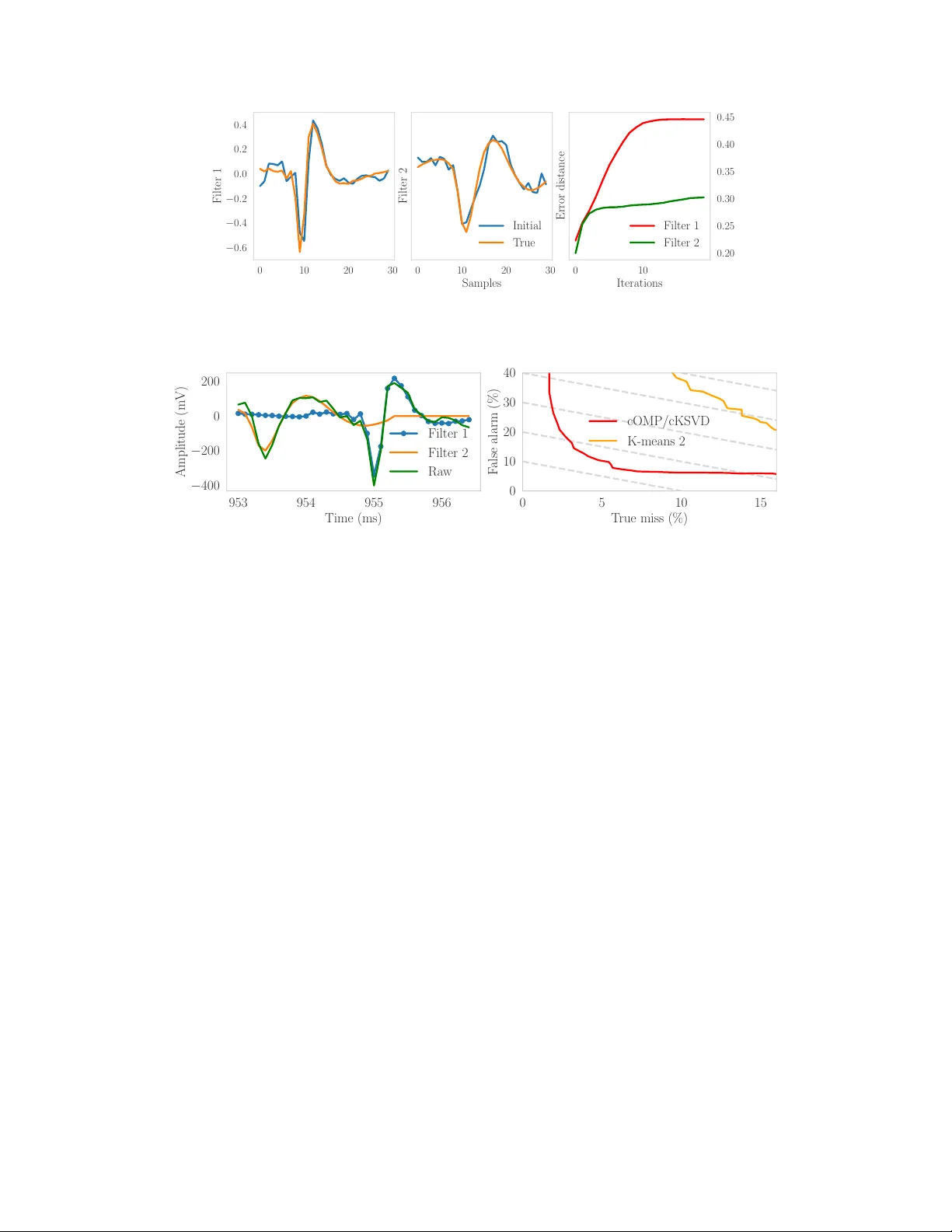
Spike Sorting by Con volutional Dictionary Lear ning Andrew H. Song Department of EECS MIT Cambridge, MA 02139 andrew90@mit.edu Francisco Flores Department of Anesthesia, Critical Care and Pain Medicine Massachusetts General Hospital and Harvard Medical School Boston, MA 02114 fjflores@neurostat.mit.edu Demba Ba School of Engineering and Applied Sciences Harvard Uni versity Cambridge, MA 02138 demba@seas.harvard.edu Abstract Spike sorting refers to the problem of assigning action potentials observed in extra- cellular recordings of neural acti vity to the neuron(s) from which they originate. W e cast this problem as one of learning a con volutional dictionary from raw multi- electrode wa veform data, subject to sparsity constraints. In this context, sparsity refers to the number of neurons that are allowed to spike simultaneously . The con volutional dictionary setting, along with its assumptions (e.g. refractoriness) that are moti vated by the spike-sorting problem, let us giv e theoretical bounds on the sample complexity of spik e sorting as a function of the number of underlying neurons, the rate of occurrence of simultaneous spiking, and the firing rate of the neurons. W e deriv e memory/computation-efficient con volutional v ersions of OMP (cOMP) and KSVD (cKSVD), popular algorithms for sparse coding and dictionary learning respectiv ely . W e demonstrate via simulations that an algorithm that alternates between cOMP and cKSVD can reco ver the underlying spike w aveforms successfully , assuming fe w neurons spike simultaneously , and is stable in the presence of noise. W e also apply the algorithm to extra-cellular recordings from a tetrode in the rat Hippocampus. 1 Introduction In experimental neuroscience, electrophysiology using extra-cellular electrodes has been the de-facto method to record neural activity from brain. With the f alling costs of storage, a recent trend is the collection and storage of ra w extracellular neural acti vity using large electrode arrays, comprising hundreds to thousands of electrodes [ 1 ], for prolonged period of up to hours/days [ 2 ], and at high sampling rates. These dev elopments have enabled the probing of neural dynamics at large spatial and temporal scale, and hav e shown promising impro vements in spike sorting, that is, the association of action potentials from extra-cellular recordings to the neuron(s) from which the y originate. Reflecting this trend, numerous approaches for spike sorting have been introduced. They fall into two broad categories. The first approach, based on the clustering of features e xtracted from the detected spike wav eforms, has been the mainstream approach for decades [ 3 ]. The features range from simple spike characteristics, such as peak amplitude and width, to more complicated features such as principal components and w avelet coef ficients [ 4 ]. Recently introduced algorithms such as Mountainsort [ 5 ] and Spyking Circus [ 6 ] employ a similar approach, with sophisticated metrics and checks to prev ent spurious ev ents from affecting the clustering. Preprint. W ork in progress. The second approach, fairly recent compared to the first, is focused on learning (or disco vering) the signature/template wa veform from each of the neurons sensed by a gi ven electrode array , and on using these to find the location of the action potentials that best match the learned signature wav eforms. T ypically , the templates are iterati vely learned, for instance by computing a running av erage of the wa veforms classified as coming from the same neuron [ 7 ]. The Matching Pursuit algorithm [ 8 ] has been the popular method for matching the templates and identifying the neuron(s) associated with extra-cellular action potentials [6, 7, 9]. More recently , the second approach has been strengthened by drawing from the signal processing literature, particularly the sparse approximation literature [ 10 ]. A simple generativ e model for the observations from a single extra-cellular electrode is the sum of the conv olution of each spike wa veform with the marked point-process consisting of the spike times from a giv en neuron and the associated amplitude [ 11 ]. In the conte xt of this generati ve model, [ 12 , 13 ] cast the problem of learning both the spike wa veforms and the spike-time/amplitude pairs as a bi-con ve x optimization problem. This leads to an algorithm, Continuous Basis Pursuit (CBP), that alternates between a sparse-approximation step to identify spik e-times/amplitudes giv en approximate spike wa veforms, and a step that updates the spike wa veforms gi ven improv ed spike times/amplitudes from the sparse approximation step. The CBP approach is computationally demanding as it requires the solution to large-scale con v ex optimization problems. Here, we cast spike sorting as a con v olutional dictionary learning problem and propose an efficient iterati ve alternating-minimization algorithm for its solution. At each iteration, the algorithm alternates between con volutional sparse coding via conv olutional orthogonal matching pursuit (cOMP) and con volutional dictionary learning via con v olutional K-SVD (cKSVD). This follows the general philosophy of the second general approach to spike sorting described above, with the connection to dictionary learning and sparse approximation made e xplicit. The innov ations from our approach are twofold. Firstly , unlike in [ 12 , 13 ] and [ 6 , 7 , 9 ], cOMP and cKSVD le verage the con v olutional form of the linear operators to perform highly memory and computation ef ficient operations, which in their nai ve form would be very slo w applied to high-sampling-rate recordings. W e use simulated and real data, for which ground-truth intracellular data are a vailable [ 14 ], to sho w that the proposed approach is able to learn accurate spike wa veforms as well as significantly reduce misclassification errors. Secondly , framing spike-sorting as con v olutional dictionary allows us to apply results from dictionary learning theory that were de veloped only recently [ 15 ]. Specifically , under some regular assumptions that we argue are reasonable in the spike-sorting setting, we giv e a theoretical bound for the required number of samples (or recording length) to reliably estimate the spik e wav eforms of a group neurons. 2 Spike Sorting as Con v olutional Dictionary Learning 2.1 Generative model and assumptions Let n = 1 , · · · , N ∈ N + be a discrete-time index and y [ n ] denote a discrete-time signal that represents the voltage from an e xtracellular electrode recording neural activity . The electrode is able to reliably capture the activity from C neighboring neurons, each with spike-w aveform template h c [ n ] , c = 1 , · · · , C . As is standard in the spik e-sorting literature, we assume that all the templates hav e equal length l . Letting h c = ( h c [0] , · · · , h c [ l − 1]) T , we assume without loss of generality , that k h c k 2 = 1 , ∀ c . A simple model for y [ n ] is that it consist of a linear combination of the time-shifted wa veform templates, perturbed by additiv e white noise ε [ n ] . Mathematically , we can express this model in terms of the con volution between the templates and code v ectors { x c [ n ] } C c =1 y [ n ] = C X c =1 x c [ n ] ∗ h c [ n ] + ε [ n ] , (1) where x c [ n ] = P N c i =1 x c,i δ [ n − n c,i ] , n = 0 , · · · , N − l + 1 , and we let x c = ( x c [0] , · · · , x c [ N − l + 1]) T . In practice, the signal y [ n ] is di vided into J non-ov erlapping windows, each of length W such that N = W J , and l << W << N . For notational con venience, denote the windo wed data by the matrix Y ∈ R W × J whose j th column Y j = ( y [( j − 1) W ] , · · · , y [ j W − 1]) T ∈ R W , j = 1 , · · · , J . Further let x c,j = ( x c [( j − 1)( W − l + 1)] , · · · , x c [ j ( W − l + 1) − 1]) T ∈ R W − l +1 be the code vector for neuron c in window j , j = 1 , · · · , J . For simultaneous recordings from M electrodes, we 2 partition each electrode into windo ws in a similar fashion and stack the resulting matrices to obtain Y ∈ R W × M J . Giv en Y , the goal is to estimate { h c } C c =1 and { x c,j } C,J c,j =1 that minimize an objective of choice, typically the error in reconstructing Y using the code vectors. Without additional constraints, it is well-kno wn that this is an ill-posed problem, i.e. there does not exist a unique solution. In the context of spike-sorting, ne vertheless, we can le verage the follo wing biophysical properties of neurons: 1) Refractoriness prev ents the same neuron from spiking again within a certain period ( ≈ 1 ms) and 2) the firing rate for a typical neuron is not high (except for extreme bursting periods). Mathematically , this implies that pairs of elements from x c,j that are close in position cannot both be nonzero and that the total number of nonzero elements of x c,j , denoted as N c,j = | supp ( x c,j ) | , should be small. In other words, { x c,j } C,J c,j =1 are sparse vectors. This naturally leads us to incorporate sparsity as a constraint on x c,j to restore well-posedness. Expressed in terms of the ` 0 quasi-norm, N c,j = k x c,j k 0 . The resulting constrained optimization problem is min { h c } C c =1 , { x c,j } C,J c,j =1 J X j =1    Y j − C X c =1 x c,j ∗ h c    2 2 s.t. C X c =1 k x c,j k 0 ≤ β (2) Note that the sparsity constraint in Eq. 2 alone does not enforce refractoriness. In practice, we found that enforcing refractoriness is not required explicitly , as it is a salient feature of the data. 2.2 Generative model with con v olutional dictionary formulation In what follows, it will be useful to express Eq. 2 in terms of the con volutional dictionary H generated by the templates { h c } C c =1 , as follows, where k·k F denotes the Frobenius norm, min H, { X j } J j =1 J X j =1    Y j − H X j    2 2 s.t. k X j k 0 ≤ β ⇔ min H,X    Y − H X    2 F s.t. k X j k 0 ≤ β (3) H ∈ R W × ( P C c =1 ( W − l +1)) is a block-T oeplitz matrix with C blocks H 1 , · · · , H C . H c is the matrix whose columns consist of all possible timeshifts of h c , zero-padded to hav e equal length: H = h H 1    · · ·    H C i where H c =     h c 0 · · · 0 0 h c · · · 0 . . . 0 . . . . . . 0 0 · · · h c     ∈ R W × ( W − l +1) (4) For each windo w j = 1 , · · · , J , the con volutional sparse code X j = ( x T 1 ,j , · · · , x T C,j ) T ∈ R P C c =1 ( W − l +1) is a concatenation of the code vectors { x c,j } C c =1 from all neurons. Expressing the con volution operation as a matrix multiplication allows us to seamlessly perform linear algebraic operations such as least-squares. Finally , let X = [ X 1 | · · · | X J ] ∈ R ( P C c =1 ( W − l +1)) × J be the matrix of code vectors from all neurons and all windows and X c = [ x c, 1 , · · · , x c,J ] ∈ R ( W − l +1) × J the c th block row of X corresponding to the code vectors from neuron c across all windows. 2.3 Alternating Minimization The objecti ve in Eq. 3 is noncon vex, due to the simultaneous optimization ov er H , X and the non- con ve x ` 0 constraint. A popular approach has been to alternati vely minimize the objecti ve o ver one of the variables while the other is fixed. This process is repeated until a con vergence criterion is reached. Let H ( t ) and X ( t ) denote the t th iterate of this alternating-minimization procedure, t ≥ 0 . At iteration t + 1 , the code matrix X ( t +1) is computed based on H ( t ) through a sparse coding step, after which H ( t +1) is computed using X ( t ) through a dictionary learning step. For the sparse coding step, Eq. 3 is combinatorially hard (and nonconv ex). Instead, se veral approaches solve an alternate con ve x objective, with the ` 1 norm replacing the ` 0 quasi-norm. Basis Pursuit (BP) denoising [ 16 ] and FIST A [ 17 ] are among the most popular such approaches. More recently , ADMM has been suggested as a more efficient alternati ve [18]. 3 Another line of work attempts to solve the original non-con v ex sparse-coding problem in a greedy fashion using algorithms such as Matching Pursuit (MP) [ 8 ] and Orthogonal Matching Pursuit (OMP) [19], a variant of the former . This line of approach is taken throughout this work, as e xplained next. 3 Con volutional Dictionary Lear ning by Con volutional OMP and Con volutional KSVD W e introduce con volutional OMP (cOMP) for sparse coding, and conv olutional KSVD (cKSVD) for con volutional dictionary learning. Our work distinguishes itself from [ 20 ] in the use of OMP as opposed to MP in the spare coding step. The applicability of recent results from dictionary learning theory [ 15 ] rely on results in compressiv e sensing that ha ve been pro ved for OMP but not for MP [ 21 ]. 3.1 An over view of classical OMP and KSVD cOMP and cKSVD are used at every iteration of the alternating-minimization procedure, respectiv ely for sparse coding and dictionary learning. Therefore we drop the super -script t indexing the iterates of the procedure and simply refer to H and X . Moreov er , since the sparse coding step consists of J independent sparse coding problems, we restrict our attention to the case of a single window Y j . (Sparse Coding) OMP is a so-called “greedy” algorithm that iterati vely selects columns from H to produce an approximation H ˆ X j of Y j . Let t 0 ≥ 1 be the iteration inde x of OMP . The algorithm terminates when the approximation error or the sparsity of ˆ X j reach a threshold. The inputs of iteration t 0 are i) the set S ( t 0 − 1) of columns that hav e been selected up to iteration t 0 − 1 , and ii) the residual error r ( t 0 − 1) from projecting Y j onto the span of S ( t 0 − 1) . At iteration 1, r (0) = Y j and S (0) = {∅} . Iteration t 0 of OMP selects the column from H with maximal absolute inner product with r ( t 0 − 1) . Because the residual is orthogonal to the span of S ( t 0 − 1) , a differ ent column of H is selected at every iter ation . Matching Pursuit is an alternativ e to OMP that has been used in spike sorting for template matching, specifically to determine the time of action potentials from a putative neuron in extra-cellular recordings [ 6 , 7 ]. MP is different from OMP in that, at iteration t 0 , it computes r ( t 0 ) = r ( t 0 − 1) − h H q ∗ , r ( t 0 − 1) i H q ∗ , where q ∗ = ar gmax q ∈ 1 , ··· ,C ( W − l +1) |h H q , r ( t 0 − 1) i| . Note the absence of the projection step onto columns that were selected at iterations prior to t 0 − 1 , which means that the same column can be selected multiple times throughout the algorithm. For spike sorting, this means that MP might detect a spike at the same location more than once. (Dictionary Learning) KSVD [ 22 ] is a popular dictionary learning algorithm that updates dictio- nary elements one at a time. Let h k be the column of the dictionary H being updated and x k be the k th row vector of X (It is dif ferent from X k that means k th block of X ). KSVD uses the SVD to minimize the error between a residual matrix computed from columns other than k and a rank-1 approximation that is the outer product of h k and x k . More formally , KSVD minimizes k Y − D X k 2 F =    Y − C X c =1 h c x c    2 F =     Y − C X c 6 = k h c x c  | {z } E k − h k x k    2 F (5) T o maintain the sparsity structure of x k , the columns of E k corresponding to the support of x k are extracted to form a shrunk error matrix, E R k . Finally , SVD is performed on E R k to obtain new ˆ h k and ˆ x k . K-SVD cycles through all the dictionary elements in this manner . 3.2 Sparse coding - Con volutional OMP (cOMP) The cOMP in volv es two computationally intensi ve steps, namely the inner product step h H T , r ( t 0 ) i , expressed as H T r ( t 0 ) , and the least-squares of projecting the residual on the the span of S ( t 0 − 1) . Con- sidering that H ∈ R W × ( P C c =1 ( W − l +1)) is high-dimensional since typical extra-cellular recordings 4 can last on the order of minutes, if not hours, with typical sampling rate of > 10 4 ( H z ) , the naiv e projection operation is computationally expensi ve. W e can take advantage of the con v olutional structure of H and compute the projection as a series of C cross-correlation operations as follows [23], H T r ( t 0 ) =  ( h 1 ? r ( t ) )[0] , · · · , ( h 1 ? r ( t 0 ) )[ W − l ] , · · · , ( h 2 ? r ( t 0 ) )[ W − l ] , · · · , ( h C ? r ( t 0 ) )[ W − l ]  T (6) where ? is a cross-correlation operation. Since this inv olves only C cross-correlation operations, it is much more ef ficient than the naiv e projection. Moreo ver , there is no need to store the entire matrix H in the memory , as only the filters { h c } C c =1 and r ( t 0 ) are required. For the least-squares step, we lev erage the fact that S ( t 0 − 1) and S ( t 0 ) are only different by one element and thus the projection onto the span of S ( t 0 ) can be obtained easily from that onto the span of S ( t 0 − 1) to further accelerate OMP computations [24]. 3.3 KSVD with con volutional dictionary (cKSVD) W e use the sparse codes X from the cOMP step to perform the con volutional KSVD (cKSVD) step. Moti vated by classical KSVD, we will update each h c at a time. W e denote by ˆ h c the updated v ersion of h c following cKSVD and b H c that of H c . Assuming h c is being updated,    Y − H X    2 F =    Y − H \ c X \ c − H c X c    2 2 =    E c − H c X c    2 2 (7) where H \ c ∈ R W × P j 6 = c ( W − l +1) refers to H with H c remov ed and X \ c ∈ R P j 6 = c ( W − l +1) × J refers to X with X c remov ed. The key distinction between cKSVD and classifical KSVD is as follows: since the columns of H c are the linear shifts of h c , we cannot update each column of H c independently . Instead, we need to update block-wise to ensure that b H c comprises shifted versions of ˆ h c . This is done by rearranging H \ c and the sparse codes as explained belo w . W e use X c j ∈ R W − l +1 to denote x c,j . Let us assume that X c j has s c,j nonzero coefficients, or s c,j =   supp ( X c j )   . The sparsity of X c j implies that we only need to deal with a subset of Y j , of length l × s c,j , that is influenced by h c . Stacking the rele vant observ ations within Y j , and across all J windo ws, we obtain ∈ R l × P J j =1 s c,j z }| { h Y (1) 1    · · ·    Y ( s c, 1 ) 1    · · ·    Y ( s c,J ) J i − ∈ R l × P J j =1 s c,j z }| { h H (1) \ c X \ c 1    · · · · · ·    H ( s c, 1 ) \ c X \ c 1    · · ·    H ( s c,J ) \ c X \ c J i | {z } E c − h c ∈ R P J j =1 s c,j z }| { h X (1) 1    · · ·    X ( s c, 1 ) 1    · · ·    X ( s c,J ) J i (8) where the superscript ( · ) , along with the subscript j for windo w j , denotes the corresponding segment (for Y j ) or block (for H \ c ) to nonzero X ( · ) j . W e perform SVD on E c and assign the first left singular vector as the ne w dictionary element, ˆ h c , and easily obtain b H c . The ne w sparse code, { b X ( s ) j } s c,j s =1 for j = 1 , · · · , J , is the first right singular v ector multiplied by the first singular v alue. b X j is constructed by replacing X ( s ) j by b X ( s ) j , thereby maintaining the support, supp ( b X j ) = supp ( X j ) . H ( t +1) and updated X ( t +1) are obtained after cycling through all C dictionary elements. 4 How much data does spike sorting r equire? Framing spike sorting as a (con volutional) dictionary learning problem, solved by alternating min- imization , lets us give theoretical bounds of the amount of data necessary to reliably estimate the wa veforms for a gi ven set of neurons. In this section, we impose further assumptions on the generati ve model of Equation 1 that allow us to apply results from dictionary learning theory [ 15 ]. W e make the 5 T able 1: Estimates based on theory of the complexity of spike sorting in terms of recording length. W e assume δ = 0 . 001 , and at most s = 3 neurons can spike simultaneously . ¯ λ C 5 10 20 5 45 secs. 1 min. 30 secs. 3 mins. 25 secs. 10 22 secs. 47 secs. 1 min. 42 secs. 20 11 secs. 24 secs. 51 secs. following assumptions Assumption 1: Events occur in non-o verlapping windows of length l . This assumption is one of mathematical con venience, which allo ws us to a void boundary ef fects. Mathematically , ∀ c, n c,i = ml , for some m s.t. n c,i ≤ N − l . Assumption 2: Refractoriness . Each neuron has a refractory period of at least l samples ( 1 ms), i.e. ∀ c, n c,i − n c,i − 1 6 = 0 . Under these assumptions, we can express Eq. 1 in linear-algebraic form by splitting y [ n ] into J =  N l  disjoint windows Y j = H X j , j = 1 , · · · , J (9) where Y j ∈ R l , X j ∈ R C , x j,c 6 = 0 only if neuron c has an ev ent in the j th window and H = [ h 1 | · · · | h c ] ∈ R l × C . Assumption 3: At most s neurons can spike simultaneously . This is equiv alent to assuming that X j from Eq. 9 is s -sparse ∀ j = 1 , · · · , J . If the number of neurons C > l , it would be unreasonable to hope to separate up top C neurons. Expressing Eq. 9 in matrix form, i.e. Y = H X , let AltMinDict( Y , H (0) ,  0 ) denote the alternating minimization algorithm for dictionary learning from [ 15 ]. Under Assumptions 1–3 , and the in the absence of noise in Eq. 1, alternating between cOMP and cKSVD reduces to AltMinDict( Y , H (0) ,  0 ). W e hav e the following result re garding the complexity of spike sorting Theorem. F or each c = 1 , · · · , C , let λ c ( t ) denote the conditional intensity function (CIF) of neur on c and N c ( t ) the associated counting pr ocess. Suppose the CIFs are uniformly bounded by ¯ λ Hz. Let 0 < δ << 1 be a pr ecision/accuracy parameter . Under assumptions A1–A7 fr om [ 15 ], with pr obability at least 1 − 2 δ , the t th iterate H ( t ) of AltMinDict( Y , H (0) ,  0 ) satisfies the following for all t ≥ 1 min z ∈{− 1 , 1 } k z h ( t ) c − h c k 2 ≤ 1 2 t  0 . (10) In particular , Assumption A5 translates into a bound on the recor ding-length complexity of spike sorting–length of r ecor ding requir ed for sorting–of T r ≥ 1 ¯ λ 4 max  C 2 s , C M 2  log  2 C δ  seconds , (11) wher e M ≈ 1 is a bound on the normalized spik e amplitudes. The theorem states that, as long as the initial dictionary is close to the true one, the error between the iterates of the alternating minimization algorithm for dictionary learning–which con v olutional cOMP/cKSVD reduce to with our assumptions abov e–and the true one will decrease exponential fast.T able 1 suggests that the theoretical estimates are very reasonable. The qualitati ve trend is that the recording length decreases linear with firing rate and increases linearly with the number of neurons. For multiple electrodes that are able to reliably detect the same neurons, the figures should be di vided by the number of electrodes. In the Supplemental Material , we re-state assumptions A1–A7 from [ 15 ], discuss their implications and how reasonable the y are in the spike-sorting conte xt, and give a sketch of a proof of the theorem. 5 A pplication to real and simulated electr ode data W e applied our method to two datasets. W e simulated the first dataset using a library of spike wa veforms obtained from extra-cellular recordings. The second dataset consists of tetrode recordings 6 0 20 40 − 0 . 4 − 0 . 2 0 . 0 0 . 2 Filter 1 T rue Initial Learned 0 20 40 samples Filter 2 0 20 40 Filter 3 0 10 20 T rue miss (%) 0 . 0 2 . 5 5 . 0 7 . 5 10 . 0 12 . 5 15 . 0 F alse alarm (%) Filter 1 Filter 2 Filter 3 Figure 1: (Left) Dictionary recovery of true templates for the simulated data with SNR 6 dB, with initial template perturbation error distance of 0.4 (Right) False alarm and T rue miss rate for each filter as the amplitude threshold is v aried. The x marker indicates the best K-means 3 cluster result, in terms of the sum of error rates. from the rat Hippocampus with simultaenous intracellular recording [ 14 ]. For both, we performed 20 iterations of cOMP & cKSVD for the dictionary learning step. Follo wing dictionary learning, we used cOMP for spike sorting and standard clustering with K-means as a benchmark. For both data sets, the inputs to the K-means algorithm use snippets of the signal, that cross a pre-computed threshold, projected onto the lower dimensional space spanned by the 10 principal components of the snippet matrix with largest singular v alue. These accounted for 90 % of the v ariance [3, 13]. 5.1 Simulated Data: Recov ery of the true templates W e simulated data with three spike wa veform templates, each 45 samples long. The data consist of 50 windows, each 3 × 10 4 samples long (equiv alent to 1 second with 30 kHz sampling rate). In a single window , the firing rate of each neuron was 40 Hz and modulated to hav e peak amplitude distributed uniformly in [ − 75 , − 125] ( mV ) . W e enforced refractoriness by pre venting wa veforms from the same neurons from ov erlapping. Finally , we added Gaussian noise with v ariance corresponding to a desired Signal-to-Noise ratio (SNR). W e initialized the dictionary learning algorithm by perturbing the three templates with additiv e noise to achie ve an av erage error distance er r ( ˆ h, h ) = max c q 1 − h h c , ˆ h c i 2 equal to 0 . 4 , where h c and ˆ h c as the column c of the two dictionaries of interest, and k h c k 2 = k b h c k 2 = 1 , ∀ c . Fig.1 shows the true/initial/recov ered templates after 20 iterations of cOMP & cK-SVD. The figure show that the algorithm performs exact recovery of the true templates for varying lev els of SNR. The learned templates all con verged to error distances of less than 10 − 2 from the true ones. W e also perturbed both the signal and the initial dictionary with higher noise v ariance and v erified that the templates were recov ered (results not shown here). 5.2 Simulated Data: Recov ery of the true sparse codes (spike-sorting) Next, we assessed ho w well cOMP was able to sort spikes from the simulated data at varying le vels of SNR. W e terminate cOMP when the residual error goes belo w the noise lev el that perturbed the signal. W e assessed the performance based on two error statistics: The “T rue miss rate" is the proportion of true spikes not identified. The “False alarm" rate is the proportion of identified spikes that are not true spikes. W e assess the rates for the individual templates separately . The error rates were assessed as a function of amplitude threshold, where the crossing of the threshold indicates identification of the recov ered wav eform as a spike. For noisy data (6 dB), Fig.1 shows that cOMP/cKSVD is able to reduce both error criteria significantly compared to an algorithm that assigns spik es to one of the three clusters found by K-means with K = 3 . 7 0 10 20 30 − 0 . 6 − 0 . 4 − 0 . 2 0 . 0 0 . 2 0 . 4 Filter 1 0 10 20 30 Samples Filter 2 Initial T rue 0 10 Iterations 0 . 20 0 . 25 0 . 30 0 . 35 0 . 40 0 . 45 Error distance Filter 1 Filter 2 Figure 2: (Left) Initial and learned dictionary for the real data for C = 2 . (Right) The error distance betwen the initial and the learned dictionary as a function of iterations. 953 954 955 956 Time (ms) − 400 − 200 0 200 Amplitude (mV) Filter 1 Filter 2 Ra w 0 5 10 15 T rue miss (%) 0 10 20 30 40 F alse alarm (%) cOMP/cKSVD K-means 2 Figure 3: (Left) Example of how cOMP decomposes the raw signal into sum of two learned wav eforms. (Right) The false alarm and true miss rate for cOMP/cKSVD and K-means with 2 clusters with varying threshold. 5.3 Extra-cellular data from tetr ode in rat Hippocampus W e filtered the data with a highpass filter at 400 H z to remove the slo w drift. Additionally , 0.9 second of data with anomalous bursting activities w as removed. The cOMP termination criterion was estimated to be the standard deviation of the background noise extracted from a segment that remains below a pre-defined threshold for more than 500 (ms). This automated approach is more appealing than ones in which hyperparameters of the algorithm are manually tuned [6, 7, 13]. W e ran cOMP/cKSVD for C = 2 . For the initialization of the templates (30 samples), we randomly picked the C segments of the signal that crossed the threshold that were as distant from each other as possible, in terms of the error distance defined previously . Fig.2 and Fig.3 show the result for C = 2 . The error distance displayed is that between the initial and the learned dictionary , and is expected to increase as the dictionary is learned. The fact that the error stabilizes after a certain number of iterations indicates that it has learned a set of templates that is deemed optimal. The true miss of < 2 % (in Fig.3) in cOMP/cKSVD, which is a significant improvement o ver the K-means algorithm, is comparable to e xisting methods. Finally , Fig.3 is an example demonstrating that a shifted linear combination of templates is able to reconstruct the raw signal accurately . 6 Conclusion W e hav e cast the spike-sorting problem in the framework of con volutional dictionary learning and showed that it can be solv ed efficiently through an iterati ve procedure that alternates between con volutional OMP and conv olutional KSVD, generalizations respecti vely of OMP and KSVD. The framing of spike sorting as a con volutional dictionary learning problem, and its solution via alternating minimization, let us employ recent theoretical results in the field of dictionary learning that gi ve estimates on the length of recordings required for spik e sorting. In future work, we will 1) massiv ely parallelize the sparse coding step with GPU architecture, 2) generalize our framew ork to 8 two dimensions to process multi-electrode recordings where the spatial extent of the areas must be considered and 3) deriv e improv ed theoretical bounds for conv olutional dictionary learning. 9 References [1] Hernan Gonzalo Rey , Carlos Pedreira, and Rodrigo Quian Quiroga. Past, present and future of spike sorting techniques. Brain Resear c h Bulletin , 119:106–117, 2015. [2] Ashesh K. Dhawale, Rajesh Poddar , Stef fen B.E. W olff, V alentin A. Normand, Evi Kopelo witz, and Bence P . Ölveczk y . Automated long-T erm recording and analysis of neural activity in behaving animals. eLife , 6:1–40, 2017. [3] Michael Lewicki. A revie w of methods for spike sorting: the detection and classification of neural action potentials. Network: Computation in Neural Systems , 9(4):R53–R78, 1998. [4] R. Quian Quiroga, Z. Nadasdy , and Y . Ben-Shaul. Unsupervised Spike Detection and Sorting with W avelets and Superparamagnetic Clustering. Neural Computation , 16(8):1661–1687, 2004. [5] Jason E. Chung, Jeremy F . Magland, Alex H. Barnett, V anessa M. T olosa, Angela C. T ooker , Kye Y . Lee, Kedar G. Shah, Sarah H. Felix, Loren M. Frank, and Leslie F . Greengard. A Fully Automated Approach to Spike Sorting. Neur on , 95(6):1381–1394.e6, 2017. [6] Pierre Yger, Giulia LB Spampinato, Elric Esposito, Baptiste Lefeb vre, Stéphane Den y , Christophe Gardella, Marcel Stimberg, Florian Jetter , Guenther Zeck, Ser ge Picaud, Jens Duebel, and Olivier Marre. A spike sorting toolbox for up to thousands of electrodes validated with ground truth recordings in vitro and in viv o. eLife , 7:e34518, mar 2018. [7] Marius Pachitariu, Nicholas A. Steinmetz, Shabnam N. Kadir , Matteo Carandini, and K enneth D. Harris. Fast and accurate spike sorting of high-channel count probes with KiloSort. In Advances in Neural Information Pr ocessing Systems 30 , 2016. [8] S. G. Mallat and Zhifeng Zhang. Matching pursuits with time-frequency dictionaries. IEEE T r ansactions on Signal Pr ocessing , 41(12):3397–3415, Dec 1993. [9] Jinhyung Lee, Da vid Carlson, Hooshmand Shokri, W eichi Y ao, Georges Goetz, Espen Hagen, Eleanor Batty , EJ Chichilnisky , Gaute Einev oll, and Liam Paninski. Y ass: Y et another spike sorter . In Advances in Neural Information Pr ocessing Systems , 2017. [10] J. A. T ropp and A. C. Gilbert. Signal recov ery from random measurements via orthogonal matching pursuit. IEEE T ransactions on Information Theory , 53(12):4655–4666, Dec 2007. [11] Maneesh Sahani, John S. Pezaris, and Richard A. Andersen. On the separation of signals from neighboring cells in tetrode recordings. In M. I. Jordan, M. J. K earns, and S. A. Solla, editors, Advances in Neural Information Pr ocessing Systems 10 , pages 222–228. MIT Press, 1998. [12] Chaitanya Ekanadham, Daniel T ranchina, and Eero P Simoncelli. A blind sparse deconv olution method for neural spike identification. In Advances in Neural Information Pr ocessing Systems , pages 1440–1448, 2011. [13] Chaitanya Ekanadham, Daniel Tranchina, and Eero P . Simoncelli. A unified framew ork and method for automatic neural spike identification. Journal of Neur oscience Methods , 222:47–55, 2014. [14] D a Henze, Z Borhegyi, J Csicsvari, A Mamiya, K D Harris, and G Buzsáki. Intracellular features predicted by extracellular recordings in the hippocampus in vi vo. Journal of neur ophysiology , 84(1):390–400, 2000. [15] Alekh Agarwal, Animashree Anandkumar , Prateek Jain, and Praneeth Netrapalli. Learning Sparsely Used Overcomplete Dictionaries via Alternating Minimization. SIAM Journal on Optimization , 26(4):2775–2799, 2016. [16] Scott Shaobing Chen, Da vid L Donoho, and Michael A Saunders. Atomic Decomposition by Basis Pursuit *. SIAM REVIEW c Society for Industrial and Applied Mathematics , 43(1):129– 159, 2001. [17] Amir Beck and Marc T eboulle. A fast iterativ e shrinkage-thresholding algorithm for linear in verse problems. SIAM journal on imaging sciences , 2(1):183–202, 2009. [18] Cristina Garcia-Cardona and Brendt W ohlber g. Con volutional dictionary learning. arXiv pr eprint arXiv:1709.02893 , 2017. [19] Y . C. P ati, R. Rezaiifar , and P . S. Krishnaprasad. Orthogonal matching pursuit: recursiv e function approximation with applications to wavelet decomposition. In Pr oceedings of 27th Asilomar Confer ence on Signals, Systems and Computers , pages 40–44 vol.1, 1993. 10 [20] Arthur Szlam, Koray Kavukcuoglu, and Y ann LeCun. Con volutional matching pursuit and dictionary training. CoRR , abs/1010.0422, 2010. [21] Joel A T ropp and Anna C Gilbert. Signal recovery from random measurements via orthogonal matching pursuit. IEEE T ransactions on information theory , 53(12):4655–4666, 2007. [22] Michal Aharon, Michael Elad, and Alfred Bruckstein. K-SVD: An algorithm for designing ov ercomplete dictionaries for sparse representation. IEEE T ransactions on Signal Pr ocessing , 54(11):4311–4322, 2006. [23] C. Zhang, D. Florencio, D. E. Ba, and Z. Zhang. Maximum lik elihood sound source localization and beamforming for directional microphone arrays in distributed meetings. IEEE T ransactions on Multimedia , 10(3):538–548, April 2008. [24] Ron Rubinstein, Michael Zibule vsky , and Michael Elad. Efficient implementation of the k-svd algorithm using batch orthogonal matching pursuit. Cs T echnion , 40(8):1–15, 2008. 11 7 Supplemental Material 7.1 Assumptions A1–A7 from [15] (A1) Dictionary Matrix satisfying RIP : The dictionary matrix H has 2 s -RIP constant of δ 2 s < 0 . 1 . (A2) Spectral Condition of Dictionary Elements: The dictionary matrix has bounded spectral norm, for some constant µ 1 > 0 , k H k 2 < µ 1 C l . (A3) Non-zero Entries in Coefficient Matrix : The non-zero entries of X are drawn i.i.d. from a distribution such that E [( X c j ) 2 ] = 1, and satisfy the following a.s.: | X c j | ≤ M , ∀ , c, j . (A4) Sparse Coefficient Matrix : The columns of the coef ficient matrix have s non-zero entries which are selected uniformly at random from the set of all s -sized subsets of { 1 , · · · , C } . It is required that s ≤ l 1 / 6 c 2 µ 1 / 3 1 , for some univ ersal constant c 2 . (A5) Sample Complexity : For some univ ersal constant c 3 = 4 , and a given failure parameter δ > 0 , the number of samples J needs to satisfy J ≥ c 3 max ( C 2 , C M 2 s ) log  2 C δ  . (12) (A6) Initial dictionary with guaranteed error bound : It is assumed that we ha ve access to an initial dictionary estimate H (0) such that max c ∈{ 1 , ··· ,C } min z ∈{− 1 , 1 } k z h (0) c − h c k 2 ≤ 1 2592 s 2 . (13) (A7) Choice of Parameters for Alternating Minimization : AltMinDict( Y , H (0) ,  0 ) uses a sequence of accuracy parameters  0 = 1 2592 s 2 and  t +1 = 25050 µ 1 s 3 √ l  t . (14) Interpr etation of A1–A7 for spike sorting . W e now discuss the appropriateness of these assump- tions in the spike-sorting setting. As with most theoretical results, the theorem provides a set of guidelines that appear reasonable (T able 1) 1. A1 requires the RIP constant of order 2 s for H to be smaller than a small v alue. Loosely , this states that subset of colums of H of size 2 s , i.e. subsets of the C neural templates of order 2 s should be dissimilar . This is an assumption that is hard to satisify in spike sorting because the neural templates can be very similar . The authors in [ 15 ] relax the RIP assumption to incoherence, i.e. an upper bound of the inner-product between pairs of neural templates. The lar ger this upper bound, the smaller then number of neurons that can spike simultaneously while guaranteeing exact reco very . The bound for the incoherent case is of the same form as that abov e. Suppose M ` ≤ | X c j | ≤ M u = M , the main dif ference is that one has to pay a factor  M u M `  2 as opposed to M 2 , i.e. a factor proportional to the ration of the maximum to the minimum normalized spike amplitudes. Assuming the spike amplitude distribution is f airly concentrated around some mean (high SNR), this is negligible. 2. A2 is a reasonable assumption on the largest eigen value of H from Eq. 9. 3. A3 can be generalized to requiring that the amplitudes of the coef ficients E [( X c j ) 2 ] = σ 2 x i.e. ha ve bounded v ariance, and an upper bound on the absolute v alue of the coefficients nor - malized by their standard deviation, i.e. | X c j | σ 2 x ≤ M , assumptions which are also reasonable in the spike-sorting setting. 4. A4 requires that only a few neurons are allowed spike simultaneously . Loosely , it states that s 3 ∝ l 1 / 2 . 5. A5 giv es the sample complexity that guarantees that, with the stated probability , the bound from the theorem holds. The form of the bound comes from the concentration results from random matrix theory used in [ 15 ] to prov e the result that alternating minimization succeeds with high probability for dictionary learning. 12 6. A6 states that the initial dictionary should be close to the true one, an assumption which is reasonable in spike sorting. 7. W e can re-write the matrix form of Eq. 9 as follows Y = H X = H ( t ) X + ( H − H ( t ) ) X . W e can treat the second term, that comes from approximating H with H ( t ) , as noise. A7 states that, as the iterations of cOMP and cKSVD proceed, we should decrease the noise lev el in OMP , which is reasonable. In practice, this did not affect results much in the high SNR case. 7.2 Proof of Theor em W e giv e a sketch of a proof of the Theorem stated in the main manuscript. Pr oof. The theorem follo ws from applying Theorem 1 from [ 15 ]. Under assumptions A1–A7, this giv es a bound for J ≥ 4 max ( C 2 , C M 2 s ) log  2 C δ  , i.e. the sample complexity of spike-sorting cast as dictionary learning (under our assumptions abo ve). J corresponds to the number of windows of length l for which at least one of the neurons spikes. W e can turn this into a recording-length complexity by upper bounding the rate of occurrence of the ev ent “at least one of the neurons spikes”. Let λ ( t ) denote the rate of occurrence of said ev ent. In an interval of width ∆ = 1 ms, we can use a union bound argument to upper bound the probability of the event V = {∪ C c =1 V c } , V c = { N c ( t + ∆) − N c ( t ) = 1 } in terms of the CIFs of the neurons and ∆ P [ V ] ≤ C X c =1 P [ V c ] = C X c =1 λ c ( t )∆ ≤ s ¯ λ ∆ , (15) where s comes from the fact that we alllo w at most s neurons to spike at the same time. Therefore, by definition of the CIF , λ ( t ) = lim ∆ → 0 P [ V ] ∆ ≤ s ¯ λ , yielding the recording-length complexity J s ¯ λ , as stated in the theorem. 13