A Generalized Matrix Inverse with Applications to Robotic Systems

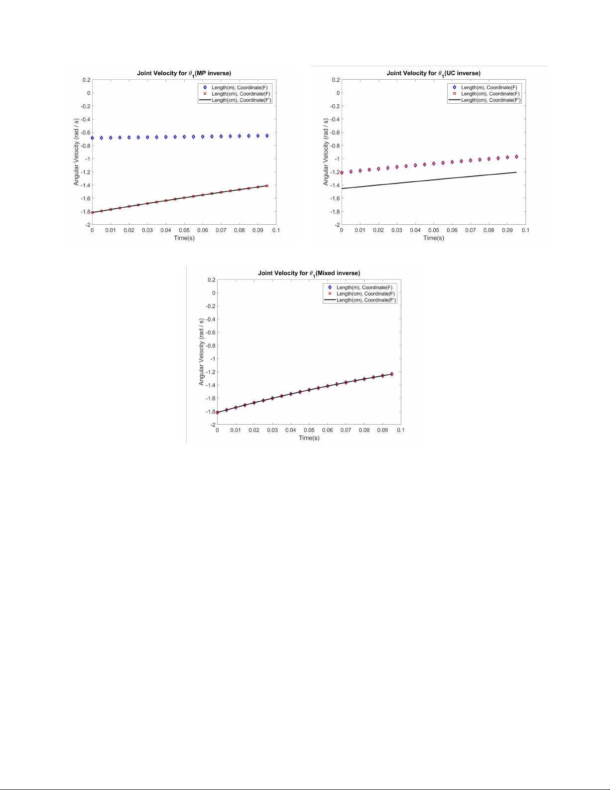
1 A Generalized Matrix In v erse with Applications to Robotic Systems Bo Zhang and Jef frey Uhlmann Dept. of Electrical Engineering & Computer Science Uni versity of Missouri-Columbia Abstract It is well-understood that the robustness of mechanical and robotic control systems depends critically on minimizing sensitivity to arbitrary application-specific details whenev er possible. For example, if a system is defined and performs well in one particular Euclidean coordinate frame then it should be expected to perform identically if that coordinate frame is arbitrarily rotated or scaled. Similarly , the performance of the system should not be affected if its key parameters are all consistently defined in metric units or in imperial units. In this paper we show that a recently introduced generalized matrix in verse permits performance consistency to be rigorously guaranteed in control systems that require solutions to underdetermined and/or overdetermined systems of equations. Keyw ords : Control Systems, Generalized Matrix In verse, Inv erse Problems, Linear Estimation, Linear Systems, Moore-Penrose Pseudoin verse, System Design, UC Generalized In verse, Unit Consistency . I . I N T RO D U C T I O N Many robotic and mechatronic control systems are mathematically represented, analyzed, and ultimately implemented as compositions of linear systems. This is the case ev en if the dynamics of the system are fundamentally nonlinear but are solved in terms of linear-algebraic equations or locally-linear approximations within globally nonlinear state-space models. In such systems it is commonly necessary to solve an overdetermined or underdetermined set of equations in order to satisfy a giv en set of constraints or to select from a multiplicity of local solutions within an iterative process. Although this may happen in a single step of a logically small component of a very large system, if care is not taken to ensure that critical mathematical properties are properly preserved the integrity of the overall system can be compromised. It is a fundamental design principal that sensitivity to arbitrary application-specific details should be minimized whenever possible. For example, if a system is defined and performs well in some particular Euclidean coordinate frame then it should be expected to perform identically if that coordinate frame is arbitrarily rotated or scaled. Similarly , the performance of the system should not be affected if its key parameters are all consistently defined in metric units or in imperial units. In this paper we sho w that a recently introduced generalized matrix inv erse permits performance consistency to be rigorously guaranteed in control systems that require solutions to underdetermined and/or overdetermined systems of equations. Specifically , we sho w that consistency with respect to arbitrary choices of units in state-space models of robotic systems can be affected by a simple replacement of the Moore-Penrose generalized matrix inv erse with a general unit-consistent in verse. I I . G E N E R A L I Z E D M A T R I X I N V E R S E S For a nonsingular n × n matrix A there exists a unique matrix in verse, A − 1 , which preserves many properties that hold for ordinary scalar inv erses, e.g., matrix in version distributes over nonsingular multiplicands as: ( X AY ) − 1 = Y − 1 A − 1 X − 1 (1) where noncommutativity of matrix multiplication imposes a constraint on the ordering of terms but is otherwise analogous to the scalar case. In a practical application the above inv erse-distributi vity property implies that if we only have access to A from its inv erse in a linearly transformed space, S = ( X AY ) − 1 , then A can be obtained simply as Y S X . When attempting to generalize the notion of a matrix in verse for singular A it is only possible to define an approximate in verse A ∼ -1 that retains a subset of the algebraic properties of a true matrix in verse [1], such as: AA ∼ -1 A = A (2) and A ∼ -1 AA ∼ -1 = A ∼ -1 (3) and/or other properties that may be of analytic or application-specific utility . The Moore-Penrose pseudoin verse [2], [3] (MP in verse), A − P , is by far the most widely known and used generalized inv erse 1 . It is defined for any m × n matrix A and 1 The Matlab/Octave operator pinv(M) returns the MP inv erse of its matrix argument. 2 satisfies the above generalized in verse properties as well as the following for any conformant unitary/orthonormal 2 matrices U and V : ( U AV ) − P = V ∗ A − P U ∗ (4) This property implies that the MP in verse is applicable to problems defined in a Euclidean state space for which the behavior of the system of interest should be inv ariant with respect to arbitrary rotations of the coordinate frame. In that context A can be recovered from its MP in verse in a rotationally transformed space as A = V ( U AV ) − P U , where consistency with respect to rigid rotations has been implicitly exploited. This can be understood by noting that if A is singular it must be assumed that A 6 = Y ( X AY ) − P X for arbitrary nonsingular matrices X and Y . More technically , the MP in verse is consistent with respect to arbitrary unitary transformations but not to general linear transformations. Despite its widespread default use throughout most areas of engineering (often implicitly under the name “ least-squar es ”), the MP in verse does not satisfy conditions appropriate for many problems to which it is commonly applied, e.g., ones that require consistency with respect to the choice of units for state variables. For example, a state parameterized with four variables defined respectively in units relating to temperature, pressure, speed, and distance can be thought of as defining a 4-dimensional Cartesian coordinate frame, but it would make no sense to rotate that coordinate frame to a space in which these variables are mixed. In this case consistency should be preserved with respect to changes of units, e.g., from imperial to metric, rather than with respect to rotations of a global coordinate frame which has no physical meaning or interpretation. This kind of unit consistency (UC) requires a generalized in verse A ∼ -1 that satisfies ( D AE ) ∼ -1 = E − 1 A ∼ -1 D − 1 (5) where the diagonal matrix D represents units on variables in one space and the diagonal matrix E represents dif ferent units for the same variables in a different space. The hazards associated with the misuse of the MP in verse hav e been noted in the robotics literature [4], [5], and disciplined methodologies hav e been de veloped to address the issue in common situations that arise in that context [6], [7]. Howe ver , the recent deriv ation of an inherently unit-consistent generalized inv erse, or UC inv erse, reduces the need for tailored solutions because in principle it can be simply substituted in place of the MP in verse [8]. This is not only useful because it simplifies the implementation process, it also reduces the opportunity for subtle implementation errors to be introduced. In the next section we e xamine a robotic system in which we demonstrate that the MP in verse fails to preserve unit consistency and thus produces unreliable results. W e then show that simply replacing the MP in verse with the UC inv erse provides improved and completely stable behavior that is in variant with respect to arbitrary changes of units on key parameters. I I I . G E N E R A L I Z E D M A T R I X I N V E R S E F O R R O B O T I C S S Y S T E M In this section we consider an example inv olving the motion of a robotic arm. This example is based on systems that hav e been studied in the literature to show the important aspects of real-world robotics and mechanical system applications [7], [9]. W e will start by describing the structure of the robotic arm and the equations that model its motion so that it can be controlled to perform desired operations. The components and configuration of the robotic arm are shown in Figure 1. It has structures common in mechanical systems. The tip-point P A is the end-effector , which denotes the end of a robotic arm and designed to interact with the outside en vironment. Each joint can be actuated by a motor , and due to the design of the connection, it is limited to 2-dimensional planar motion. The mechanism has 3 degrees of freedom: two of them are rotational and one is linear . These parameters are initialized as θ 1 = 30 ◦ , θ 2 = 30 ◦ and l = 0 . 7 m . A mixed control of these joints will determine the motion of tip-point P A , e.g., to take it to a desired state B. T aking the cylindrical joint on the frame as the origin, the position of the tip-point P A ( [ x, y , z ] ) is gi ven by equations 6-8. x = a 1 c 1 + a 2 c 12 + l · s 12 (6) y = a 1 s 1 + a 2 s 12 − l · c 12 (7) z = 0 (8) where s 1 = sin( θ 1 ) , c 1 = cos( θ 1 ) , s 12 = sin( θ 1 + θ 2 ) , c 12 = cos( θ 1 + θ 2 ) . A Jacobian matrix represents the transformation of the end-effector representation of the dynamic system ( P A ) into a joint-state representation in which all of the key parameters are represented as a vector as q . For the current problem the state of the system is given by q = [ θ 1 , θ 2 , l ] T , which are the states of the 3 joints. The Jacobian matrix for this system, J = ∂ P A ∂ q (9) 2 For notational purposes we retain the generality of interpreting U and V as arbitrary unitary matrices over C or H (e.g., U − 1 is equal to its conjugate transpose U ∗ ), but for all practical purposes in this paper they can be thought of as representing permutations of state variables and/or rotations of a global coordinate frame. 3 Fig. 1: Robotic arm system with two rotational joints and one linear joint. The tip-point P A is the end-effector designed to interact with the environment. is determined to be   − a 1 s 1 − a 2 s 12 + l · c 12 , − a 2 s 12 + l · c 12 , s 12 a 1 c 1 + a 2 c 12 + l · s 12 , a 2 c 12 + l · s 12 , − c 12 0 , 0 , 0   The target velocity is thus J = ∂ P A ∂ q = ∂ P A ∂ t · ∂ t ∂ q (10) ∂ P A ∂ t = J ∂ q ∂ t (11) or ~ v = J ˙ q (12) where ~ v is the deriv ative of P A , and ˙ q is the joint velocity of the robotic arm represented by ˙ q = [ ˙ θ 1 , ˙ θ 2 , ˙ l ] T . Assuming a target velocity ~ v = [2 , − 2 , 0] T ( m/s ) , the solution to achieve the desired motion is ˙ q = J − 1 ~ v (13) but this cannot be evaluated if J is singular , and it will be singular in this case because the motion is constrained to a 2-dimensional plane in a 3-dimensional space. The solution therefore requires use of a generalized matrix in verse in place of the undefined matrix in verse. As has been discussed, the most commonly used generalized in verse is the Moore-Penrose (MP) in verse, which giv es a result for ˙ q as ˙ q = J − P ~ v (14) where J − P is the MP in verse. As will be seen, the use of the MP inv erse is not appropriate if the state vector has variables with units that must be preserved, which is true for the case of q . In this system lengths are defined in meters, a 1 = 1 m , a 2 = 1 . 1 m , l = 0 . 7 m , and ~ v = [2 , − 2 , 0] T ( m/s ) , though the system should be expected to work correctly no matter what 4 T ABLE I: Joint velocity of robotic arm calculated using MP inv erse. T imestep: 0.001s. T ime( s ) ˙ θ 1 ( deg ree/s ) ˙ θ 2 ( deg ree/s ) ˙ l ( m/s ) V T ( m/s ) 0.000 -27.881 -12.12 -1.543 [2, -2, 0] 0.001 -27.826 -11.981 -1.548 [2, -2, 0] 0.002 -27.772 -11.838 -1.553 [2, -2, 0] 0.003 -27.719 -11.695 -1.558 [2, -2, 0] 0.004 -27.666 -11.552 -1.563 [2, -2, 0] 0.005 -27.614 -11.409 -1.568 [2, -2, 0] 0.006 -27.563 -11.266 -1.573 [2, -2, 0] 0.007 -27.513 -11.123 -1.578 [2, -2, 0] 0.008 -27.464 -10.980 -1.582 [2, -2, 0] 0.009 -27.414 -10.837 -1.587 [2, -2, 0] 0.010 -27.367 -10.693 -1.592 [2, -2, 0] Fig. 2: T ip point position after simulation, solved with MP in verse. (a) length unit(m), timestep ( 10 − 3 s ). (b) length unit(cm), timestep ( 10 − 3 s ). (c) length unit(cm), timestep ( 10 − 4 s ). Simulation (b) fails by deviating from designed track. units are used as long as everything is defined consistently in those units. The joint velocity needed to keep the speed of tip-point P A equal to ~ v is calculated using equation 14 with timesteps of dt = 10 − 3 s over a simulation time of 0.1 s. At each timestep (e.g., t = 0 s, t = 10 − 3 , t = 2 × 10 − 3 ) the angles and lengths are updated for the next iteration as q (1) = q (0) + ˙ q (0) · dt so that the Jacobian matrix can also be updated to solve the ˙ q for the next timestep. The calculated velocities included in T able I can be seen to change slowly over time, and the simulation shows that they lead to a tip-point velocity that is approximately equal to ~ v during the process. The final state of the tip-point is sho wn in Figure 2(a), which sho ws that the target was successfully controlled to move along the designed track. In contrast to the first simulation, the second simulation is performed identically except that lengths are defined in units of centimeters instead of meters: a 1 = 100 cm , a 2 = 110 cm , l = 70 cm , and ~ v = [200 , − 200 , 0] T ( cm/s ) . As a result, some elements of the Jacobian matrix are changed in magnitude, b ut the ov erall behavior of the system should be expected to remain unchanged. In other words, as long as ev erything is implemented consistently using lengths defined in meters, or implemented consistently using lengths defined in centimeters, the behavior of the system should be the same because the controls will be computed accordingly . The choice of units should not matter , and if it does then the system cannot be trusted. Although the joint velocities are calculated the same way as before with a timestep of 10 − 3 s , the system now di ver ges rapidly . For example, Figure 3(a) shows that the value of the angular velocity θ 1 rapidly fluctuates between [ − 2000 , 2000] r ad/s , whereas the computed angular velocity in the previous simulation remained stable at around 30 r ad/s . Figure 2(b) sho ws that the control is unsuccessful as the tip-point motion di verges from the designed path. T o reduce the magnitude of this deviation the control system has to be performed using much smaller timesteps, which requires control operations to be calculated and applied much more frequently to keep the tip from di verging too far from the correct path. The results of sev eral tests are plotted in Figure 3. It can be seen that acceptable results are obtained with a timestep of 10 − 3 s when lengths are defined in units of meters, but unstable results are produced when the length unit is changed to centimeters. In the centimeter case it is necessary to reduce the timestep by an order of magnitude to 10 − 4 s to achiev e reliable control, but this increases the computational complexity by an order of magnitude because control operations must be calculated much more frequently . While this does yield an acceptable tip-point velocity , the control values are dif ferent from those produced when units were in meters and this is evidence that something is wrong. It is tempting to conclude based on the final state displayed in Figure 2(c) that the controls perform equally well in both cases because they produce seemingly similar paths. Howe ver , Figure 3(a) shows that the control produced in the case of centimeter units leads to very erratic high-frequency motion along the path, and the controls required to achiev e these wildly changing velocities may be physically difficult to actually achiev e 5 (a) (b) (c) (d) Fig. 3: Joint velocity ( ˙ θ 1 ) solved with MP in verse. (a) length unit(cm), timestep ( 10 − 3 s ). (b) length unit(cm), timestep ( 10 − 4 s ). (c) length unit(cm), timestep ( 10 − 5 s ). (d) length unit(m), timestep ( 10 − 3 s ). Simulation (a) does not con ver ge, and simulation (b) and (c) can conv erge with a smaller timestep. with real hardware. Even if they can be achie ved they may cause excessi ve stress and wear on machine elements. The simulations clearly show that different units lead to different configurations for the same problem when using the MP in verse. The final state of the robotic arm is θ 1 = 27 . 379 ◦ , θ 2 = 29 . 483 ◦ and l = 0 . 875 m for lengths in meters, θ 1 = 22 . 109 ◦ , θ 2 = 38 . 129 ◦ and l = 0 . 864 m for lengths in centimeters. The fact that results depend on the choice of units raises concerns because there is no way to predict when and how this dependency may lead to bad results. Although the timestep can be reduced until the controls calculated using the MP in verse produce acceptable results, the need to adjust the timestep to compensate for arbitrary dependencies on the choice of units implies that the solution has been tailored to the problem and the results may not remain acceptable for a slightly different configuration. Therefore, this control system using the MP in verse cannot be trusted. It is important to re view why the control system in this case seemed to work well when units were defined in meters but not when they were defined in centimeters. This happened because the control calculations used the MP in verse when there was need to inv ert a singular Jacobian matrix. Based on the properties discussed in the previous chapter , the MP inv erse is defined to provide a solution to a linear system Ax = y that minimizes the Euclidean norm || Ax − y || 2 for an over -constrained system, or to minimize the norm || x || 2 for an under-constrained system. While this makes sense for vectors in which elements are all defined in the same Euclidean coordinate system, it does not make sense when the elements (parameters) are not defined in a common coordinate frame and hav e incommensurate units. This is because the choice of units affects the magnitude of “error” that is contributed by each element when the sum of squared errors is minimized. For our case the MP in verse attempts to minimize || ˙ q || 2 = ˙ θ 2 1 ( deg ree 2 /s 2 ) + ˙ θ 2 2 ( deg ree 2 /s 2 ) + ˙ l 2 ( m 2 /s 2 ) (15) where the relativ e contributions of dif ferent terms clearly depend on the arbitrary choices of units for the different elements. This shows that squared-error is not a physically meaningful quantity to minimize when different variables are defined in different units. The loss of physical meaning when minimizing Euclidean inner products in volving v ariables with incommensurate units has been observed to be problematic for robotic systems [4], [6], and essentially the same problem applies in our case when the MP in verse is applied to the Jacobian matrix representing the transformation of variables in incommensurate units. This is why our simulation results were not consistent with respect to changes of units from meters to centimeters. The fact that 6 minimizing squared error has no physical meaning in this context reinforces the conclusion that the calculated controls using the MP inv erse should not be trusted. At this point it is valuable to consider what property of a generalized in verse is needed to avoid the unit dependency problems of the MP in verse. What is needed is a solution that is consistent with respect changes of units in the governing equation Ax = y , which can be expressed in the form of diagonal matrices D and E as x 0 = D x (16) y 0 = E y (17) where x 0 is just x but with elements defined in different units and y 0 is similarly obtained from y . The gov erning equation can now be expressed as y 0 = E Ax = E AD − 1 x 0 (18) The solution can be expressed in terms of an unknown generalized inv erse ( E AD − 1 ) f − 1 as x 0 = E Ax = ( E AD − 1 ) f − 1 y 0 (19) while the solution in the original units was x = A f − 1 y = A f − 1 E − 1 y 0 . In order to satisfy our assumption that changes of units take the form of diagonal transformations, e.g., x 0 = D x and y 0 = E y , the unknown general inv erse must satisfy ( E AD − 1 ) f − 1 = D A f − 1 E − 1 (20) which is not satisfied by the MP inv erse because it only provides consistency with respect to orthogonal transformations (rotations) but not diagonal transformations. The problem to be solved requires a generalized inv erse that ensures consistency for diagonal transformations, and an in verse of this kind has been recently dev eloped [10]. This unit-consistent (UC) in verse can be defined in terms of the MP in verse as follows: A − U = ( D A S E A ) − U (21) = E − 1 A S − P D − 1 A (22) where D A and E A are positive diagonal matrices determined from A , and S is a matrix uniquely determined from A so that the magnitude of the product of the nonzero elements of each row and column of S is 1. (The basis for this decomposition, and its existence and uniqueness properties, are described in [10].) The UC inv erse works by eliminating the effect of diagonal transformations. From the definition it can be seen that A − U = ( D − 1 A D A AE A E − 1 A ) − U (23) = E A ( D A AE A ) − P D A (24) So for any diagonal matrices D and E applied to change the units, ( E AD − 1 ) − U = ( E D − 1 A D A AE A E − 1 A D − 1 ) − U (25) and since E − 1 A D − 1 and E D − 1 A are also diagonal matrices: ( E AD − 1 ) − U = ( E − 1 A D − 1 ) − 1 ( D A AE A ) − P ( E D − 1 A ) − 1 (26) = D E A ( D A AE A ) − P D A E − 1 (27) = D A − U E − 1 . (28) This sho ws that the UC in verse satisfies the consistency requirement of equation 20. The problems we hav e demonstrated with the MP in verse occur because it does not produce control behavior that is in variant with respect to the choice of units. Assuming the motion is giv en as ~ v m = J m ˙ q m in units of meters, with the Jacobian matrix terms giv en in equation 9 and ~ v m = [ ~ v x , ~ v y , ~ v z ] T , the transformation of units from meters to centimeters, ~ v cm = J cm ˙ q cm , can be expressed as a diagonal transformation in the form of:   c, 0 , 0 0 , c, 0 0 , 0 , c   · ~ v m = J m ·   c, 0 , 0 0 , c, 0 0 , 0 , 1   · ˙ q cm (29) where c = 100 is the scale factor of conv erting from meters to centimeters. What is needed is a generalized in verse that will guarantee inv ariance with respect to units. The UC in verse has this property , so we should expect that using it in place of the MP in verse will eliminate unit dependencies in the control calculations and a void the unstable beha vior demonstrated in our earlier simulations. This can be tested simply by re-running the simulations with the MP in verse replaced by the UC 7 Fig. 4: Joint velocity ( ˙ θ 1 ) generated by simulations using both length units(meter / centimeter) and timestep ( 10 − 3 s ). The result changes smoothly over the simulation time. in verse and checking whether the performance of the control system is in variant with respect to changes of units from meters to centimeters. Said another way , changing the units should produce a control solution defined in the new units but which exhibits the exact same physical behavior obtained using the original units. As was done in the earlier simulations, controls are calculated with a timestep of 10 − 3 s over a simulation time of 0 . 1 s for the case of lengths defined in meters and then with lengths in centimeters according to equation 14. Figure 4 sho ws that in both cases the control produced using the UC inv erse con verges rapidly , and the velocity variation is identically smooth in both cases. This corroborates our expectation that the UC in verse produces stable results that are not affected by the arbitrary choice of units used for lengths. It should be noted that we sho wed in the earlier simulations that the timestep could be reduced so that controls from the MP in verse also produced acceptable results. The difference is that the UC-in verse solution mathematically guarantees that its results are in variant with respect to the choice of units and therefore does not require timestep changes to av oid unpredictable behaviors. The MP in verse does not hav e the correct mathematical properties and therefore cannot offer the same guarantee. I V . G E N E R A L I Z E D C O N S I S T E N C Y C O N S I D E R A T I O N S In the previous section it was sho wn that the UC in verse satisfied all requirements for maintaining unit consistency in the example system 3 . In this secton we examine how the UC in verse can also be combined with the MP in verse, and e ven other generalized in verses (e.g., the Drazin in verse [11], [12], [13] or other similarity-consistent inv erse [15]), to construct solutions to in verse problems when there is a mix of variables inv olving different consistency requirements. In addition to variables that require unit consistency to be preserved, a complex real-world system may also inv olve v ariables defined in a Cartesian coordinate frame that require consistency with respect to rotations of that coordinate frame. In other words, the behavior of the control system must be in variant with respect to changes of units for some variables and in variant with respect to rotations for other variables. The UC in verse is applicable in one case while the MP in verse is applicable in the other, but what is needed for such a system is a generalized in verse that will guarantee unit consistency for some variables and rotation consistency for others. If we assume 4 that the first m variables require unit consistency and the remaining n variables require rotation consistency then the transformation matrix to be in verted can be block-partitioned as A =  W X Y Z  } m } n |{z} m |{z} n (30) It has been shown [10] that the mixed in verse can be obtained from this block-partitioned form as A − M =  ( W − X Z -P Y ) -U − W -U X ( Z − Y W -U X ) -P − Z -P Y ( W − X Z -P Y ) -U ( Z − Y W -U X ) -P  (31) 3 An additional property that is sometimes required of a generalized in verse that was not demonstrated in our example system is consistency with respect to use of the Kronecker product. Because this property was not among those established in [10], we formally prove it in Appendix A. 4 The ordering of the variables is arbitrary so there is no loss of generality in assuming they are permuted so that the UC variables come first and the rotation-consistent variables come next. 8 (a) (b) (c) Fig. 5: Rover with an extendable arm. The rover is free to move on a plane, body part B can ascend/descend or rotate, and the arm can be extended. The two projected views, D 1 and D 2 , show the structure of the arm. θ 0 = 45 ◦ is a fixed angle. The coordinate frame F 0 is a rotation of the original frame F by an angle of θ 0 . In the previous examples it has been stressed that the problem solution should not depend on arbitrary system preferences because such dependencies lead to unpredictable results. In the case of a system with a mix of consistency requirements we should expect the correct solution to produce the same behavior if units on the first m variables are changed or if the coordinate frame of the remaining n variables is rotated. If the mixed in verse above is correct then the controls produced should have this property . W e will demonstrate that it does in the following example. Consider the control of a planetary rov er with a robotic arm as displayed in Figure 5, which includes two projected vie ws in directions D 1 and D 2 . The x-y coordinate is shown as frame F . The frame F 0 , which is an orthogonal transpose of frame F by θ 0 , will be considered later . The rover is free to move in any direction on planar terrain, and its Cartesian position coordinates in this plane are ( x 1 , y 1 ) . The part B can rotate and can also ascend/descend 5 . In addition, the arm can elongate within a fixed range, but it cannot rotate in the vertical plane. Thus there are 5 degrees of freedom for the design, denoted as q = [ θ 1 , l, x 1 , y 1 , z 1 ] T , where ( x 1 , y 1 , z 1 ) is the position coordinates of part B. From the geometry relations, the position of tip-point P A is gi ven as P A = [ x, y , z , 0 , 0] T , x = x 1 + l · sin θ 0 · cos θ 1 (32) y = y 1 + l · sin θ 0 · sin θ 1 (33) z = z 1 − l · cos θ 0 (34) W e can use the same approach of the previous example to generate the Jacobian matrix for ~ v = J ˙ q as 5 The part B can be thought of as an extendible arm for taking a soil or rock sample. This rover , called ODIF , is intended to function as part of a team of lightweight bots for large area inv estigation. 9 J =       − l · sin θ 0 sin θ 1 sin θ 0 cos θ 1 1 0 0 l · sin θ 0 cos θ 1 sin θ 0 sin θ 1 0 1 0 0 − cos θ 0 0 0 1 0 0 0 0 0 0 0 0 0 0       The initial states are set to be θ 1 = 45 ◦ and l = 1 . 0 m , the constant angle θ 0 = 45 ◦ . The target velocity of the tip-point is ~ v = [2 , 0 , − 1 , 0 , 0] m/s . Since the system has redundant degrees of freedom and therefore J is singular, ˙ q = J f − 1 ~ v has to be solved with a general inv erse (e.g. MP in verse, UC in verse, or mixed inv erse). For the unknown variables in ˙ q , [ ˙ θ 1 , ˙ l ] hav e incommensurate units, and [ ˙ x 1 , ˙ y 1 , ˙ z 1 ] are defined in a common Euclidean space. Thus the Jacobian matrix can be partitioned as W =  − l · sin θ 0 sin θ 1 sin θ 0 cos θ 1 l · sin θ 0 cos θ 1 sin θ 0 sin θ 1  , X =  1 0 0 0 1 0  Y =   0 − cos θ 0 0 0 0 0   , Z =   0 0 1 0 0 0 0 0 0   Now the mixed inv erse can be used to find the solution for ˙ q using equation 31. W e initially use meters as the length unit and F as the coordinate frame. W e will then consider a change of length units from meters to centimeters and a coordinate frame rotation from F to F 0 by a rotation angle of θ 0 = 30 ◦ . Giv en c = 100 as the scale factor to con vert from meters to centimeters, the gov erning equation for the centimeter and rotated case, ~ v cm,F 0 = J cm,F 0 ˙ q cm,F 0 , can be expressed as a diagonal transformation of the meter case, ~ v m,F = J m,F ˙ q m,F , as       c cos( θ 0 ) , − c sin( θ 0 ) , 0 , 0 , 0 c sin( θ 0 ) , c cos( θ 0 ) , 0 , 0 , 0 0 , 0 , c, 0 , 0 0 , 0 , 0 , c, 0 0 , 0 , 0 , 0 , c       · ~ v m,F =       cos( θ 0 ) , − sin( θ 0 ) , 0 , 0 , 0 sin( θ 0 ) , cos( θ 0 ) , 0 , 0 , 0 0 , 0 , 1 , 0 , 0 0 , 0 , 0 , 1 , 0 0 , 0 , 0 , 0 , 1       · J m,F ·       c, 0 , 0 , 0 , 0 0 , 1 , 0 , 0 , 0 0 , 0 , 1 , 0 , 0 0 , 0 , 0 , 1 , 0 0 , 0 , 0 , 0 , 1       · ˙ q cm,F 0 This shows the block of the matrix requiring rotation consistency and the block of variables defined in incommensurate units. W e then test the three possible approaches to computing the controls: using the MP in verse alone; using the UC in verse alone; and using the mixed in verse obtained from equation 31. The solutions for ˙ q from the three approaches are displayed in table II for t = 0 s . The column headings give the unit/coordinate frame in which each test was performed but the results are all given in (con verted to) a common coordinate frame for comparison purposes. As can be seen, the mixed inv erse is the only approach that produces identical results regardless of coordinate-system changes. For the other approaches, it can be seen that when the controls are ev aluated with the MP inv erse, it generates the same results when different coordinate frames are used but not when length units are changed. When the UC in verse is solely applied to the entire system it generates in variant solutions when units are changed but not when rotations are applied. Therefore, it can be concluded that solely using either the UC in verse or MP in verse alone will not produce reliable results. Instead, the mixed in verse is required to ensure that the behavior of the system is inv ariant with respect to defined changes of units and coordinates. A transient simulation was performed for 0 . 1 s to further observe the full control process. Figure 6(a) displays variation of θ 1 for the three approaches. It shows that the angular velocity calculated over time by the MP inv erse is not affected by a rotation of the coordinate frame from F to F 0 but is affected by a change of the length unit from meters to centimeters; and the rev erse is true for the UC inv erse. By contrast, the angular velocity from the mixed in verse is identical over time in all cases. In summary , for this system in volving v ariables with dif ferent consistency requirements the mixed in verse yields reliable control while the alternativ es do not. This demonstrates the necessity of using the appropriate in verse to satisfy all applicable consistency requirements. 10 T ABLE II: Joint velocities ˙ q = [ ˙ θ 1 ( r ad/s ) , ˙ l ( m/s ) , ˙ x 1 ( m/s ) , ˙ y 1 ( m/s ) , ˙ z 1 ( m/s )] T , solved with MP in verse, UC in verse, and Mixed in verse approaches. Length unit( m ) Length unit( cm ) Length unit( cm ) Coordinate( F ) Coordinate( F ) Coordinate( F 0 ) MP in v ˙ q =         − 0 . 6854 0 . 8536 1 . 1963 − 0 . 0498 − 0 . 3964         ˙ q =         − 1 . 8179 0 . 8536 0 . 5734 − 0 . 5731 − 0 . 3964         ˙ q =         − 1 . 8179 0 . 8536 0 . 5734 − 0 . 5731 − 0 . 3964         UC in v ˙ q =         − 1 . 2121 1 . 3536 0 . 6566 − 0 . 0101 − 0 . 0429         ˙ q =         − 1 . 2121 1 . 3536 0 . 6566 − 0 . 0101 − 0 . 0429         ˙ q =         − 1 . 4545 1 . 5690 0 . 3676 − 0 . 1943 − 0 . 1095         Mixed in v ˙ q =         − 1 . 8182 2 . 7071 − 0 . 3536 − 0 . 3536 0 . 9142         ˙ q =         − 1 . 8182 2 . 7071 − 0 . 3536 − 0 . 3536 0 . 9142         ˙ q =         − 1 . 8182 2 . 7071 − 0 . 3536 − 0 . 3536 0 . 9142         V . D I S C U S S I O N In this paper we discussed the fact that different generalized in verses have different properties and that the correct one must be chosen based on the properties needed for the problem at hand. For example, the MP in verse is appropriate if the application requires the behavior of the system to be in variant with respect to rotations of the coordinate frame. W e then described that many problems require the behavior of the system to be in variant with respect to the choice of units used for key parameters. For example, the behavior should be the same regardless of whether the parameters are defined in metric units or imperial units as long as all parameters are defined consistently with whatev er choice of units is made. W e emphasized that the Moore-Penrose (MP) pseudoinv erse does not satisfy this requirement. W e demonstrated what can happen if the wrong generalized in verse is used by examining the MP in verse in an example of a robotic arm in which consistency with respect to units is required. In that example it was sho wn that the MP in verse produced different behaviors depending on the choice of units, and as a result it produced erratic and unpredictable behaviors. This is because the MP inv erse provides consistency with respect to rotations rather than changes of units. W e described that methods are kno wn to tailor such problems by hand so that unit consistency can be maintained, but those methods are complicated and thus are more likely to introduce accidental errors. W e explained that what is truly needed to solve such problems is a generalized in verse that is unit consistent. Such an in verse, called the UC in verse, has recently been dev eloped, and we showed that simply replacing the MP in verse with the UC in verse does in fact eliminate all dependencies on the choice of units. Use of the UC inv erse led our example system to exhibit stable behavior in all cases. Lastly we demonstrated that the UC and MP in verses can be combined to provide consistency for systems defined with a mix of variables, some of which demand unit consistency while others require rotational consistency . A P P E N D I X A U C I N V E R S E A N D T H E K RO N E C K E R P R O D U C T The Kronecker product is often used for the mathematical representation of a complex system in terms of simpler subsys- tems [14]. In this appendix we show that the UC inv erse satisfies the same useful properties as the MP inv erse with respect to the Kronecker product. 11 (a) (b) (c) Fig. 6: Joint velocity for θ 1 solved with different generalized inv erse approaches. (a) MP in verse. (b) UC inv erse. (c) mixed in verse. Only the mixed in verse yields the same results over the 0 . 1 s for the transformations in all three cases. The Kronecker product is a non-commutative tensor operator , usually denoted as ⊗ , which takes an m × n matrix and a p × q matrix and constructs a composition of the two matrices to produce a higher-dimensional mp × nq matrix. The definition of the Kronecker product of A m × n and B p × q is A ⊗ B =      a 1 , 1 B a 1 , 2 B · · · a 1 ,n B a 2 , 1 B a 2 , 2 B · · · a 2 ,n B . . . . . . . . . . . . a m, 1 B a m, 2 B · · · a m,n B      Thus each a i,j B is a of p × q matrix. For example, assuming A is 2 × 2 and B is 3 × 2 (i.e., m = n = 2 and p = 3 , n = 2 ) then A ⊗ B =         a 1 , 1 b 1 , 1 a 1 , 1 b 1 , 2 a 1 , 2 b 1 , 1 a 1 , 2 b 1 , 2 a 1 , 1 b 2 , 1 a 1 , 1 b 2 , 2 a 1 , 2 b 2 , 1 a 1 , 2 b 2 , 2 a 1 , 1 b 3 , 1 a 1 , 1 b 3 , 2 a 1 , 2 b 3 , 1 a 1 , 2 b 3 , 2 a 2 , 1 b 1 , 1 a 2 , 1 b 1 , 2 a 2 , 2 b 1 , 1 a 2 , 2 b 1 , 2 a 2 , 1 b 2 , 1 a 2 , 1 b 2 , 2 a 2 , 2 b 2 , 1 a 2 , 2 b 2 , 2 a 2 , 1 b 3 , 1 a 2 , 1 b 3 , 2 a 2 , 2 b 3 , 1 a 2 , 2 b 3 , 2         The Kronecker product is important in engineering design because it can be used to elegantly and efficiently represent complex systems as compositions of simpler subsystems. It finds applications in control systems, signal processing, image processing, 12 semidefinite programming, and quantum computing[16], [17], [14], [18], [19], [20], [21]. It is bilinear and associative: A ⊗ ( B + C ) = A ⊗ B + A ⊗ C (35) ( A + B ) ⊗ C = A ⊗ C + B ⊗ C (36) ( k A ) ⊗ B = A ⊗ ( k B ) = k ( A ⊗ B ) (37) ( A ⊗ B ) ⊗ C = A ⊗ ( B ⊗ C ) (38) and it satisfies the following with respect to the transpose (and conjugate-transpose) operator ( A ⊗ B ) T = A T ⊗ B T (39) For matrices A, B , C and D for which the products AC and B D are valid, the following mixed-product property (so-called because it inv olves both standard matrix multiplication and the Kronecker product) can be shown to hold: ( A ⊗ B )( C ⊗ D ) = ( AC ) ⊗ ( B D ) (40) If matrices A and B are orthogonal then A ⊗ B is also orthogonal: ( A ⊗ B ) T ( A ⊗ B ) = I (41) It is also the case that ( A ⊗ B ) − 1 = A − 1 ⊗ B − 1 (42) and more generally ( A 1 ⊗ A 2 ⊗ · · · ⊗ A n ) − 1 = A − 1 1 ⊗ A − 1 2 ⊗ · · · ⊗ A − 1 n (43) The last two properties are necessary to construct a matrix to transform from one Kronecker-constructed matrix to another Kronecker -constructed matrix, which is required for performing controls of the kinds of robotic and mechanical systems of interest in this thesis, but we also require the ability to apply generalized matrix inv erses in the case of singular matrices. It has been proven that the MP in verse satisfies [22]: ( A ⊗ B ) − P = A − P ⊗ B − P (44) and more generally: ( A 1 ⊗ A 2 ⊗ · · · ⊗ A n ) − P = A − P 1 ⊗ A − P 2 ⊗ · · · ⊗ A − P n (45) but it has not yet been established that these two results also hold for the UC in verse. They must be proven in order to show that the UC in verse can be used for general control systems represented using Kronecker products. W e begin by proving that the Kronecker product of two diagonal matrices is also diagonal. Giv en diagonal matrices A and B A =      a 1 , 1 0 · · · 0 0 a 2 , 2 · · · 0 . . . . . . . . . . . . 0 0 · · · a m A ,m A      , B =      b 1 , 1 0 0 · · · 0 0 b 2 , 2 0 · · · 0 . . . . . . . . . . . . . . . 0 0 0 · · · b m B ,m B      the Kronecker product C = A ⊗ B =      a 1 , 1 B 0 · · · 0 0 a 2 , 2 B · · · 0 . . . . . . . . . . . . 0 0 · · · a m A ,m A B      can be seen to also be diagonal because every nonzero element of A is at position [ i, i ] ( 1 ≤ i ≤ m ), every nonzero element of B is at position [ j, j ] ( 1 ≤ j ≤ p ), and e very nonzero element of C is at position [ i ( p − 1) + j, i ( p − 1) + j ] . Or more simply , e very diagonal block of C is a diagonal matrix and therefore C must be a diagonal matrix. W ith these basic properties in mind, we have the prerequisites to prov e the UC in verse property . First consider the base case, A − U 1 ⊗ A − U 2 = ( A 1 ⊗ A 2 ) − U (46) 13 Recall the decomposition of equation 21 for any matrix A , where for notational clarity we now use D and E instead of D A and E A : A = D · S · E (47) and the UC generalized inv erse of A is defined as: A − U = E − 1 · S − P · D − 1 (48) Applying this to the left hand side of equation 46 giv es A − U 1 ⊗ A − U 2 = ( E − 1 1 · S − P 1 · D − 1 1 ) ⊗ ( E − 1 2 · S − P 2 · D − 1 2 ) (49) = ( E − 1 1 ⊗ E − 1 2 )( S − P 1 ⊗ S − P 2 )( D − 1 1 ⊗ D − 1 2 ) (50) = ( E 1 ⊗ E 2 ) − 1 ( S − P 1 ⊗ S − P 2 )( D 1 ⊗ D 2 ) − 1 (51) Using the fact that S − P 1 ⊗ S − P 2 = ( S 1 ⊗ S 2 ) − P giv es A − U 1 ⊗ A − U 2 = ( E 1 ⊗ E 2 ) − 1 ( S 1 ⊗ S 2 ) − P ( D 1 ⊗ D 2 ) − 1 (52) and the right-hand side of equation 46 is ( A 1 ⊗ A 2 ) − U = [( D 1 · S 1 · E 1 ) ⊗ ( D 2 · S 2 · E 2 )] − U (53) = [( D 1 ⊗ D 2 )( S 1 ⊗ S 2 )( E 1 ⊗ E 2 )] − U (54) where D 1 ⊗ D 2 and E 1 ⊗ E 2 are diagonal matrices. In order to apply equation 48, the ro ws and columns of S 1 ⊗ S 2 must satisfy the ± 1 product constraint. Let S 1 and S 2 be represented as S 1 =      a 1 , 1 a 1 , 2 · · · a 1 ,n 1 a 2 , 1 a 2 , 2 · · · a 2 ,n 1 . . . . . . . . . . . . a m 1 , 1 a m 1 , 2 · · · a m 1 ,n 1      S 2 =      b 1 , 1 b 1 , 2 · · · b 1 ,n 2 b 2 , 1 b 2 , 2 · · · b 2 ,n 2 . . . . . . . . . . . . b m 2 , 1 b m 2 , 2 · · · b m 2 ,n 2      where for any 1 ≤ i 1 ≤ m 1 , 1 ≤ j 1 ≤ n 1 , 1 ≤ i 2 ≤ m 2 , 1 ≤ j 2 ≤ m 2 , the matrix elements of S 1 and S 2 hav e the following property: Y a i 1 ,k = ± 1 ( a i 1 ,k 6 = 0) (55) Y a k,j 1 = ± 1 ( a k,j 1 6 = 0) (56) Y b i 2 ,k = ± 1 ( b i 2 ,k 6 = 0) (57) Y b k,j 2 = ± 1 ( b k,j 2 6 = 0) (58) For ev ery row i 1 ( m 2 − 1) + i 2 of S 1 ⊗ S 2 =      a 1 , 1 S 2 a 1 , 2 S 2 · · · a 1 ,n 1 S 2 a 2 , 1 S 2 a 2 , 2 S 2 · · · a 2 ,n 1 S 2 . . . . . . . . . . . . a m 1 , 1 S 2 a m 1 , 2 S 2 · · · a m 1 ,n 1 S 2      14 the product of its nonzero elements is (when a i 1 ,k 1 6 = 0 , b i 2 ,k 2 6 = 0 ) Y ( a i 1 ,k 1 ( Y b i 2 ,k 2 )) (59) = Y ( a i 1 ,k 1 ( ± 1)) (60) = Y ( a i 1 ,k 1 ) Y ( ± 1) (61) = Y ( ± 1) (62) = ± 1 . (63) The same holds analogously for every column of S 1 ⊗ S 2 , so equation 48 can be applied to equation 54 to obtain ( D 1 ⊗ D 2 )( S 1 ⊗ S 2 )( E 1 ⊗ E 2 )] − U = ( E 1 ⊗ E 2 ) − 1 ( S 1 ⊗ S 2 ) − P ( D 1 ⊗ D 2 ) − 1 (64) and from equation 52 the following theorem can be concluded: Theorem 1: A − U 1 ⊗ A − U 2 = ( A 1 ⊗ A 2 ) − U . W e no w show that Theorem 1 can be used as the base case for a mathematical induction proof of the general case in volving matrices A 1 ...A n . Gi ven ( A 1 ⊗ A 2 ⊗ · · · ⊗ A n ) − U = A − U 1 ⊗ A − U 2 ⊗ · · · ⊗ A − U n (65) it is required to show ( A 1 ⊗ A 2 ⊗ · · · ⊗ A n +1 ) − U = A − U 1 ⊗ A − U 2 ⊗ · · · ⊗ A − U n +1 (66) T o simplify the equation, let B = A 1 ⊗ A 2 ⊗ · · · ⊗ A n . Then ( A 1 ⊗ A 2 ⊗ · · · ⊗ A n +1 ) − U = ( B ⊗ A n +1 ) − U (67) A − U 1 ⊗ A − U 2 ⊗ · · · ⊗ A − U n +1 = B − U ⊗ A − U n +1 . (68) Applying Theorem 1 while Letting A 1 = B and A 2 = A n +1 we obtain ( B ⊗ A n +1 ) − U = B − U ⊗ A − U n +1 (69) from which we can expand to obtain the desired final result: Theorem 2: ( A 1 ⊗ A 2 ⊗ · · · ⊗ A n +1 ) − U = A − U 1 ⊗ A − U 2 ⊗ · · · ⊗ A − U n +1 Theorems 1 and 2 complete the set of UC inv erse properties necessary to allow it to be used in place of the MP in verse in mechanical and robotic systems whenever unit consistency is required. A P P E N D I X B I M P L E M E N T A T I O N O F U C I N V E R S E The follo wing Octav e/Matlab implementation is adapted from code in [10]. function Ai = uinv(A) tolerance = 1e-22; [m, n] = size(A); L = zeros(m, n); M = ones(m, n); S = sign(A); A = abs(A); idx = find(A > 0.0); L(idx) = log(A(idx)); idx = setdiff(1 : numel(A), idx); L(idx) = 0; A(idx) = 0; M(idx) = 0; r = sum(M, 2); c = sum(M, 1); u = zeros(m, 1); v = zeros(1, n); sumv = 0.0; prev = 1.0; while (abs(prev - sumv) > tolerance) idx = c > 0; p = sum(L(:, idx), 1) ./ c(idx); 15 L(:, idx) = L(:, idx) - repmat(p, m, 1) . * M(:, idx); v(idx) = v(idx) - p; idx = r > 0; p = sum(L(idx, :), 2) ./ r(idx); L(idx, :) = L(idx, :) - repmat(p, 1, n) . * M(idx, :); u(idx) = u(idx) - p; prev = sumv; sumv = var(sum(L)); end Ai = pinv(exp(L) . * S) . * (exp(u) * exp(v))’; end R E F E R E N C E S [1] Ben-Israel, Adi; Greville, Thomas N.E., “Generalized in verses: Theory and applications, ” New Y ork: Springer , 2003. [2] E.H. Moore, “On the Reciprocal of the general algebraic matrix, ” Bulletin of the American Mathematical Society , 26 (9): 394-395, 1920. [3] R. Penrose and J. T odd, “ A generalized in verse for matrices”, Mathematical Proceedings of the Cambridge Philosophical Society , vol. 51, no. 03, p. 406, 1955. [4] J. Duffy , “The fallac y of modern hybrid control theory that is based on orthogonal complements’ of twists and wrenches spaces”, Int. J. Robot. Sys. , 7(2), pp. 139-144, 1990. [5] C. Melchiorri, “Considerations about the use of minimum norm criteria in the solution of kinematic problems”, A CC San Diego , 1990. [6] Keith L. Doty , Claudio Melchiorri, Claudio Boniv ento, “ A Theory of Generalized In verses Applied to Robotics, ” The International Journal of Robotics Resear ch , 12(1), pp.1-19, 1993. [7] E. Schwartz, R. Manseur , K. Doty , “Noncommensurate Systems in Robotics, ” International Journal of Robotics and Automation , 17(2), 2002. [8] Jeffrey Uhlmann, “Unit Consistency , Generalized In verses, and Effecti ve System Design Methods, ” arXiv:1604.08476v2 [cs.N A] 11 Jul 2017 (2015). [9] Charles A. Klein, Ching-Hsiang Huang, “Revie w of Pseudoin verse Control for Use with Kinematically Redundant Manipulators, ” IEEE Tr ansactions on Systems, Man, and Cybernetics , SMC-13(3), 1983. [10] Jeffrey Uhlmann, “ A Generalized Matrix Inv erse that is Consistent with Respect to Diagonal T ransformations, ” SIAM Journal on Matrix Analysis (SIMAX), V ol. 39:3, 2018. [11] Drazin, M. P ., “Pseudo-inv erses in associativ e rings and semigroups”, The American Mathematical Monthly , 65 (7): 506-514, 1958. [12] S.L. Campbell, C.D. Meyer , and N.J. Rose, “ Applications of the Drazin In verse to Linear Systems of Differential Equations with Singular Constant Coefficients, ” SIAM Journal of Applied Mathematics , V ol. 31, No. 3, 1976. [13] B. Simeon, C. Fuhrer , P . Rentrop, “The Drazin in verse in multibody system dynamics”, Numer . Math , 64, pp. 521-539, 1993. [14] Lei Zhou, Xiao Bai, Xianglong Liu, Jun Zhou, Hancock Edwin, “Fast Subspace Clustering Based on the Kronecker Product”, [cs.LG] 15 Mar 2018. [15] Jeffrey Uhlmann, “ A Rank-Preserving Generalized Matrix Inv erse for Consistency with Respect to Similarity , ” arXiv:1804.07334v1 [cs.NA] 19 Apr 2018. [16] Charles F . V an Loan, “The ubiquitous Kronecker product”, J ournal of Computational and Applied Mathematics , vol. 123, no. 1-2, pp. 85-100, 2000. [17] A. Graham, “Kronecker Products and Matrix Calculus with Applications”, Ellis Horwood , Chichester , England, 1981. [18] Rachel Schlossman, Gray C. Thomas, Luis Sentis, “Exploiting the Natural Dynamics of Series Elastic Robots by Actuator-Centered Sequential Linear Programming”, ArXiv e-prints , 2018. [19] B Boots, G Gordon, “ A spectral learning approach to range-only SLAM”, International Confer ence on Machine Learning , 19-26, 2013. [20] L. Sabattini, C. Secchi and C. Fantuzzi, “ Achieving the desired dynamic behavior in multi-robot systems interacting with the en vironment”, 2017 IEEE International Conference on Robotics and Automation (ICRA), Singapore , pp. 2097-2102, 2017 [21] Daniel Zelazo, Antonio Franchi, Heinrich H. Blthoff, Paolo Robuffo Giordano “Decentralized rigidity maintenance control with range measurements for multi-robot systems”, The International Journal of Robotics Resear ch , 34(1), pp. 105 - 128, 2014. [22] Amy N. Langville, W illiam J. Stew art, “The Kronecker product and stochastic automata networks”, J ournal of Computational and Applied Mathematics , vol. 167, no. 2, pp. 429-447, 2004. Bo Zhang Bo Zhang received the B.S. degree in Mechanical Engineering from East China University of Science and T echnology , Shanghai, China in 2014 and is currently working toward the M.S. degree in the Electrical Engineering and Computer Science Department, University of Missouri-Columbia, MO. His research interests include kinematic systems and computational analysis. Jeffr ey Uhlmann Prof. Uhlmann is a faculty member of the Dept. of Electrical Engineering and Computer Science at the University of Missouri-Columbia. He received his doctorate in robotics from the Univ ersity of Oxford, UK, in 1995 and was a research scientist for 13 years at the Naval Research Laboratory (NRL) in W ashington, DC.