Efficient Atlasing and Search of Configuration Spaces of Point-Sets Constrained by Distance Intervals

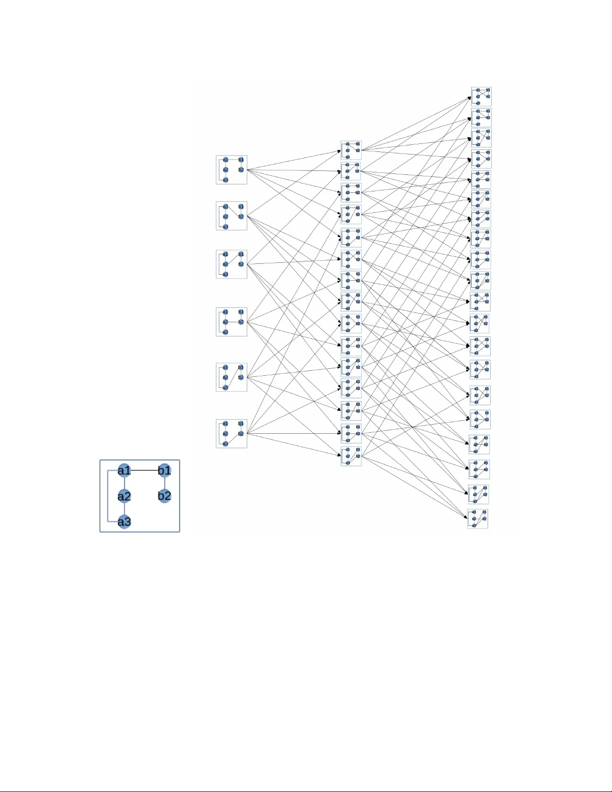
Eﬃcien t A tlasing and Searc h of Conﬁguration Spaces of P oin t-Sets Constrained b y Distance In terv als. Aysegul Ozk an, Rah ul Prabh u, T ro y Baker, James P ence, Jorg P eters and Meera Sitharam ∗ Octob er 18, 2018 Abstract F or conﬁgurations of p oin t-sets that are pairwise constrained by distance interv als, the EASAL soft- w are implements a suite of algorithms that c haracterize the structure and geometric prop erties of the conﬁguration space. The algorithms generate, describ e and explore these conﬁguration spaces using generic rigidity properties, classical results for stratiﬁcation of semi-algebraic sets, and new results for ef- ﬁcien t sampling by conv ex parametrization. The paper reviews the key theoretical underpinnings, ma jor algorithms and their implementation. The pap er outlines the main applications such as the computation of free energy and kinetics of assembly of supramolecular structures or of clusters in colloidal and soft materials. In addition, the pap er surveys select exp erimental results and comparisons. 1 In tro duction W e presen t a soft ware implementation of the algorithm EASAL (Eﬃcien t Atlasing and Search of Assem bly Landscap es) [44]. This implementation generates, describ es, and explores the feasible relative p ositions of t wo p oin t-sets A and B of size n in R 3 that are mutually constrained by distance in terv als. F ormally , a Euclidean orientation-preserving isometry T ∈ S E (3) is fe asible if, for dist a,b deﬁned as the Euclidean norm || a − T ( b ) || , the following hold: ∀ ( a ∈ A, b ∈ B ) , dist a,b ≥ ρ a,b ( C 1 ) ∃ ( a ∈ A, b ∈ B ) , dist a,b − ρ a,b ≤ δ a,b , ρ a,b , δ a,b ∈ R + . ( C 2 ) ∗ Department of Computer & Information Science & Engineering, University of Florida This research was supported in part by NSF DMS-0714912, a Universit y of Florida computational biology seed grant, NSF CCF-1117695, NSF DMS-1563234, NSF DMS-1564480 Note: 1. The EASAL softw are has tw o versions. The TOMS submission contains only the back end of EASAL, without GUI and with text input and output. The exp erimen tal results in Section 4.1 of the pap er, can b e repro duced with this version using the sample input ﬁles given i n the ﬁles directory . See Section 5 of the included TOMSUserGuide.p df for detailed instructions on how to run the test driver. An optional GUI (not part of TOMS submission) which can b e used for intuitiv e visual veriﬁcation of the results, can b e found at the EASAL rep ository . Instructions on how to install and how to use and ma jor functionalities oﬀered by the GUI are detailed in the CompleteUserGuide found in the bitbuck et respository which can b e found at http://bitbucket.org/geoplexity/easal [43]. 2. A video presenting the theory , applications, and software comp onents of EASAL is av ailable at http://www.cise.ufl. edu/ ~ sitharam/EASALvideo.mpg [48]. 3. A web version of the softw are can b e found at http://ufo- host.cise.ufl.edu (runs on Windows, Linux, and Chrome- bo oks with the latest, W ebGL 2.0 enabled go ogle chrome or mozilla ﬁrefox web browsers). 4. EASAL screen shots and movies hav e b een used in the pap ers [54, 44, 59, 53, 42, 45, 60] to illustrate deﬁnitions and theoretical results. 1 Constrain t C 1 means that T is infeasible when there exists a pair ( a, T ( b )) that is to o close. Constrain t C 2 implies that at least one pair ( a, T ( b )) is within a pr eferr e d distance in terv al. Consider for example, sets A and B of centers of non-intersecting spheres (see Fig. 2(a) and Fig. 3(a)). With ρ a , ρ b the sphere radii, the constant ρ a,b in C 1 equals ρ a + ρ b . Note that the ambien t dimension of Problem ( C 1 , C 2 ) is 6, namely , the dimension of SE(3). When T is feasible, the Cartesian c onﬁgur ation T ( B ) is called a r e alization of the constrain t system ( C 1 , C 2 ). When δ a,b ≈ 0 the eﬀective dimension of the realization space is 5. The input to EASAL consists of up to four comp onen ts. – k = 2 p oin t-sets A and B with n p oints each. (The submitted implementation is for tw o p oint-sets, but the theory and the algorithms generalize to k p oin t-sets and ambien t dimension 6( k − 1)) – The pairwise distance in terv al parameters ρ a,b , δ a,b ∈ R + . – Optional: global constraints imp osed on the ov erall conﬁguration. – Optional: a set of active constrain ts of interest. (Only constraint regions including at least one of these activ e constraints is sampled and added to the atlas.) The main output of EASAL is the dimensional, top ological and geometric structure of the r e alization sp ac e , i.e., all T ( B ) satisfying ( C 1 , C 2 ). The realization space is represented as the swe ep of the individual realizations (s ee Fig. 2(d) and Fig. 3(b)). The sw eep representation shows A together with all feasible realizations T ( B ) traced out. T o describ e this space, EASAL employs three strategies. First, EASAL partitions the realization space in to active c onstr aint r e gions , each deﬁned by the set of active c onstr aints , i.e., the pairs ( a, b ) satisfying C 2 . These pairs are edges of the active c onstr aint gr aph used to lab el the region. Suc h a graph can b e analyze d b y generic combinatorial rigidit y theory [19], in particular, the co-dimension of an active constraint region (see Section 2.1) is t ypically the num ber of active constrain t edges. Since the active constrain t regions satisfy p olynomial equations and inequalities, the realization space is semi-algebraic set (a union of sets deﬁned by p olynomial inequalities). This is the setting of a Thom-Whitney stratiﬁcation of semi-algebraic sets [38]. Second, EASAL organizes and represents the active constraint regions in a partial order (directed acyclic graph) so that the active constrain t graph of a region is a subgraph of the activ e constraint graph of its b oundary regions. This organization is called the atlas . T o construct the atlas, EASAL recursiv ely starts from the interior of an active constraint region and lo cates b oundary regions of strictly one dimension less. Suc h b oundary regions generically hav e exactly one additional activ e constrain t and the active constraint graph has one additional edge. Considering only b oundary regions of exactly one dimension less improv es robustness ov er searc hing directly for low est-dimensional regions. W e note that, when a new child region of one dimension less is found, all its higher dimensional anc estor regions are immediately discov ered since they corresp ond to a subset of the activ e constraints. Therefore, even if a region is missed at some stage, it will b e discov ered once any of its descendants are found, for example, through one of its siblings. Third, to lo cate the b oundary region satisfying an additional activ e constraint, EASAL applies the theoretical framework developed in [52]. EASAL eﬃciently maps (many to one) a d -dimensional activ e constrain t region R with active constraint graph G , to a conv ex region of R d called the Cayley c onﬁgur ation sp ac e of R . Deﬁne a non-e dge of G as a pair ( a, b ) not connected by an edge in G . The Cayley conﬁguration space of R is deﬁned intuitiv ely as the set of r e alizable lengths of d chosen non-edges of G . The v ariables represen ting these non-edge lengths are called the Cayley p ar ameters . In what follo ws, we simply refer to the non-edges as Cayley parameters. Since the Cayley conﬁguration space is conv ex, it allows for eﬃcient sampling and search. In addition, it is eﬃcient to compute the inv erse map from eac h p oint in the Ca yley conﬁguration space (a Cayley c onﬁgur ation ) to its ﬁnitely many corresp onding Cartesian realizations. The Ca yley conﬁguration space of a d -dimensional active constrain t region R is discretized and represented as a d -dimensional grid. The Ca yley p oin ts adjacen t to the low er dimensional b oundary regions of R are highligh ted in diﬀerent colors (See Fig. 2(b)). Eﬃciency , accuracy , and tradeoﬀ guarantees ha ve been formally established for EASAL (see Section 3.5). The total n umber of active constraint regions in the atlas could b e as large as O ( k 2 · n 12 k ). The maximum 2 dimension of a region is 6( k − 1). If r regions of dimension d ha ve to b e sampled, EASAL requires time linear in r and exp onen tial in d . EASAL can explore assemblies up to a million regions for smal l assemblies in a few hours on a standard laptop (see Section 4.1). By small assemblies we mean constrain t problems with n ≤ 5000 and k = 2; or n ≤ 3 and k ≤ 18. Eﬃciency can impro ve signiﬁcan tly when the p oin t-sets are iden tical, by exploiting symmetries in the conﬁguration space [54]. Section 4 surv eys n umerical exp erimen tal results from [53], for (i) generating the atlas, (ii) using the atlas to ﬁnd paths b etw een active constraint regions and (iii) using the atlas to ﬁnd the neighbor regions of an active constrain t region. W e also survey exp erimen tal results from [42], comparing the p erformance of EASAL with Metrop olis Mark o v c hain Mon te Carlo (MC) and from [60] for EASAL predicting the sensitivit y of icosahedral T=1 viruses tow ards assembly disruption. Organization: After brieﬂy reviewing applications of EASAL to molecular and materials modeling and related work, the remainder of the pap er is organized as follows. Section 2 discusses the theory underlying EASAL. Section 3 discusses the algorithmic ideas and implementation. Section 4 surv eys experimental results, Section 5 sketc hes the softw are architecture. 1.1 Application to Molecular and Materials Modeling EASAL provides a new approach to the longstanding challenges in molecular and soft-matter self-assembly under short range p oten tial in teractions. EASAL can b e used to estimate free-energy , binding aﬃnit y and kinetics. F or example, EASAL can b e applied to (a) supramolecular self-assembly or do cking starting from rigid molecular motifs e.g., helices, p eptides, ligands etc. or (b) self-assem bly of clusters of multiple particles eac h consisting of 1-3 spheres - e.g., in amphiphiles, colloids or liquid crystals. In the context of molecular assembly , rigid comp onents of the mole cules corresp ond to the input p oint- sets A and B , and atoms corresp ond to the p oin ts a ∈ A and b ∈ B . The activ e constraint regions corresp ond to regions of constant p otential energy derived from discretized Lennard-Jones [28] p otential energy terms. It is intractable or at least prodigiously exp ensive to atlas large molecular assem blies by an y naiv e global metho d. Assemblies are typically recursively decomp osed into smaller assem blies (deﬁned ab o ve) and recom bined. Generally , the input molecules ha ve a small set of interfaces (pairs of atoms, one from eac h molecule) where b ond formation is feasible. These are given as input by sp ecifying a set of active constrain ts of interest corresp onding to the interfaces. EASAL atlases only those r active constraint regions where at least one of these constraints is active (i.e., C 2 holds). 1.1.1 Geometrization of Molecular In teractions in EASAL In EASAL, the inter-atomic Lennard-Jones p oten tial energy terms are ge ometrize d in to 3 main regions: (i) large distances at which no force is exerted b etw een the atoms, suc h atom pairs, called inactive constraints, corresp ond to ( a, b ) suc h that dist a,b > ρ a,b + δ a,b , (ii) very close distances that are prohibited b y in ter- atomic repulsion or inter-atomic collisions and violating C 1 . (iii) the interv al b etw een these, known as the Lennard-Jones wel l , in which bonds are formed, corresp onding to the preferred distance or active constrain ts deﬁned in C 2 . The pairwise Lennard-Jones terms are typically input only for selected pairs of atoms, one from each rigid component. Hard-sphere steric constraints, apply to all other pairs and enforce (i) and (ii) with δ a,b = 0 in C 2 . Having more activ e constrain ts corresp onds to low er potential energy , as well as to lo wer eﬀectiv e dimension of the region. The low est p otential energy is attained at ze ro-dimensional regions, i.e., for rigid active constraint graphs and ﬁnitely many conﬁgurations. F or each rigid activ e constrain t graph G , the corresp onding p oten tial energy b asin includes w ell-deﬁned p ortions of higher dimensional regions whose activ e constraint graphs are non-trivial subgraphs of G . In this manner the Cartesian conﬁguration space is partitioned into p otential energy basins. F ree energy of a conﬁguration dep ends on the depth and w eighted relativ e volume (conﬁgurational entrop y) of its p otential energy basin. Since low est free energy corresp onds to lo west p otential energy and high relative volume of the p otential energy basin, w e are often speciﬁcally in terested in zero-dimensional regions where the p otential energy is 3 lo west. Ho wev er, the v olume of the p otential energy basins corresp onding to these regions typically include p ortions of all of their higher dimensional ancestor regions. These ancestor regions should therefore b e found and explored. Similarly , computing kinetics inv olves a comprehensive mapping of the top ology of paths b et ween regions, where the paths could pass through other regions of v arious eﬀective dimensions. Although paths w ould b e exp ected to fav or low dimensional regions since they ha ve the lo west energy , these paths could b e long, requiring many energy ups and downs, as well as backtrac king, which could cause more direct paths to b e fav ored that pass through higher dimensional, higher energy regions. EASAL (i) directly atlases and navigates the complex top ology of small assem bly conﬁguration spaces (deﬁned earlier), crucial for understanding free-energy landscap es and assem bly kinetics; (ii) a voids multiple sampling of conﬁgurational (b oundary) regions, and minimizes rejected samples, both crucial for eﬃcient and accurate computation of conﬁgurational volume and entrop y and (iii) comes with rigorously prov able eﬃciency , accuracy and tradeoﬀ guarantees (see Section 3.5). T o the b est of our knowledge, no other current soft ware provides such functionality . 1.2 Related W ork 1.2.1 Related W ork on Geometric Algorithms A generalization of Problem ( C 1 , C 2 ) arises in the rob otics motion planning literature with exp onential time algorithms to compute a roadmap (a v ersion of atlas) and paths in general semi-algebraic sets [11, 10, 4], with probabilistic versions to impro ve eﬃciency [33, 34]. F or the Cartesian conﬁguration space of non intersecting spheres, Baryshniko v et al. and Kahle characterize the complete homology [3, 29], viable only for relatively small point-sets or spheres, while more empirical computational approac hes for larger sets [12, 8] come without formal algorithmic guarantees. A geometric rigidity approach was primarily used to characterize the graph of contacts of arbitrarily large jammed sphere conﬁgurations in a b ounded region [30, 16]. Unlik e these approaches, the goal of EASAL is to describ e the conﬁguration space of Problem ( C 1 , C 2 ). In addition, EASAL is deterministic and its eﬃciency follo ws from exploiting special prop erties of those semi-algebraic sets that arise as conﬁguration spaces of p oint-sets constrained by distance interv als. 1.2.2 Related W ork on Molecular and Materials Mo deling The simplest form of supramolecular self assem bly and hence the simplest application of Problem ( C 1 , C 2 ) is site-sp eciﬁc do cking. Computational geometry , vision and image analysis hav e b een used in site-sp eciﬁc do c king algorithms [7, 15, 32, 17, 51]. Unlike the more general goals of EASAL, the goal of these algorithms is to simply ﬁnd site-speciﬁc do c king conﬁgurations with optimal binding aﬃnit y . While this dep ends on equilibrium free energy , do c king metho ds simply ev aluate an approximate free energy function. On the other hand, prev ailing metho ds for direct free energy computation - that m ust incorp orate b oth the depth and relative weigh ted volumes (entrop y) of the free energy basin - use highly general approaches suc h as Monte Carlo (MC) and Molecular Dynamics (MD) simulation. They deal with a notoriously diﬃcult generalization of Problem ( C 1 , C 2 ) [31, 1, 22, 23, 21, 36, 20, 13, 37]. Ergo dicity of these methods is unpro ven for conﬁguration spaces of high geometric or top ological complexity with low energy , low v olume regions (low eﬀective dimension) separated by high energy barriers. Hence they require unpredictably long tra jectories starting from man y diﬀeren t initial conﬁgurations to lo cate suc h regions and compute their v olumes accurately . While these metho ds are applicable to a wide v ariet y of molecular mo deling problems, they do not take adv an tage of the simpler inter-molecular constrain t structure of assembly ( C 1 , C 2 ) compared to, sa y , the in tra-molecular folding problem (see [57]): active constrain t graphs that arise in assem bly (see Fig. 4) yield con vexiﬁable conﬁguration spaces whereas the folding problem has additional ‘bac kb one’ constrain ts that prev ent conv exiﬁcation. Therefore, even though the energy functions used b y MC and MD can diﬀer in assem bly and folding, these metho ds miss out on critical adv an tages by not explicitly exploiting sp ecial geo- metric prop erties of small assemb ly conﬁguration spaces. EASAL on the other hand exploits such geometric prop erties via Cayley conv exiﬁcation. 4 W e do not review the extensiv e literature on (ab-initio) simulation or other decomposition-based metho ds that are required to tractably deal with large assemblies. F or small cluster assem blies from spheres, i.e., n = 1 and k ≤ 18, there exist a n umber of methods to compute free energy and conﬁgurational en tropy of subregions of the conﬁguration space [24, 2, 56, 5, 9, 35, 26, 25]. W orking with traditional Cartesian conﬁgurations, they m ust deal with subregions that are comparable in complexity to the entire Cartesian conﬁguration space of small molecules suc h as cyclo-octane [40, 27, 47]. With n = 3, there are b ounds for appro ximate conﬁgurational en tropy using rob otics-based metho ds without relying on MC or MD sampling [13]. F or arbitrary n and starting from MC and MD samples, recen t heuristic methods infer a topological roadmap [18, 55, 39, 49] and use top ology to guide dimensionality reduction [61]. In particular [24] formally show ed that their (and EASAL’s) geometrization is physically realistic, but, they directly search for hard-to-ﬁnd zero dimensional active constrain t regions b y w alking one-dimensional boundary regions of the Cartesian conﬁguration space. In addition they compute one and tw o dimensional volume in tegrals. T o the b est of our knowledge these metho ds do not exploit key features of assembly conﬁguration spaces that are crucial for EASAL’s eﬃciency and prov able guaran tees. These include Thom-Whitney stratiﬁca- tion, generic rigidity properties, Cayley con vexiﬁcation, and recursiv ely starting from the higher-dimensional in terior and lo cating easy-to-ﬁnd b oundary regions of exactly one dimension less. Using these and adaptive Jacobian sampling [45], EASAL can rapidly ﬁnd all generically zero-dimensional regions and can b e used to compute not only one and t wo, but also higher dimensional volume integrals [53], as well as paths that pass through m ultiple regions of v arious dimensions. This is imp ortant for free energy and kinetics computation. 1.2.3 Recen t W ork Lev eraging EASAL EASAL v ariants and traditional MC sampling of the assembly landscap e of tw o transmembrane helices ha ve recently b een compared from multiple p ersp ectiv es in order to leverage complemen tary strengths [42]. In addition, EASAL has b een used to detect assembly-crucial inter-atomic interactions for viral capsid self- assem bly [59, 60] (applied to 3 viral systems: Minute Virus of Mice (MVM), Adeno-Associated Virus (AA V), and Bromo-Mosaic Virus (BMV)). This work exploited symmetries and utilized the recursiv e decomp osition of the large viral capsid assembly in to an assembly pathw a y of smaller assem bly intermediates. Adapting EASAL to exploit symmetries was the sub ject of [54]. Though the submitted implemen tation can handle only t wo p oint-sets as input ( k = 2), for greater than 2 p oin t-sets, the extension of the EASAL algorithm and implemen tation ha v e been sho wn to be straigh tforward [44, 53]. When n = 1, i.e., eac h p oin t-set is an iden tical singleton sphere, exploiting symmetries leads to simpler computation. EASAL has b een used to compute 2 and 3 dimensional conﬁgurational v olume in tegrals for 8 assembling spheres for the ﬁrst time [53], relying on Cayley conv exiﬁcation. Building up on the current soft ware implementation of EASAL, an adaptive sampling algorithm directly leads to accurate and eﬃcient computations of conﬁgurational region volume and path integrals [45]. 2 The Theory Underlying EASAL The EASAL soft ware is based on the theoretical concepts described in this section. W e explain and illustrate EASAL’s three strategies b elow. The reader will ﬁnd the video at http://www.cise.ufl.edu/sitharam/ EASALvideo.mpg useful to understand the following. 2.1 Strategy 1: A tlasing and Stratiﬁcation EASAL’s ﬁrst strategy is to partition and stratify the Cartesian conﬁguration space into regions R called the active constrain t regions, each lab eled by its active c onstr aint gr aph (See Fig. 1(a)). Consider the set of p oints participating in the active constraints that deﬁne R . Let V R b e any minimal sup erset of p oints that supp orts additional constraints, of type C 2 , to lo cally ﬁx (generically rigidify) the tw o p oin t-sets with resp ect to each other. No w, V R is taken to b e the set of v ertices of the active constraint graph of R . An edge of the activ e constraint graph represents either (i) one of the active constraints that deﬁne R or (ii) a 5 (a) Activ e constraint graph used to lab el a 2D node in (b); ( a 1 , b 1 ) is the sole active constraint edge. (b) Stratiﬁcation DA G of Ex. T o y3. Figure 1: Atlas (stratiﬁcation) of the (toy-sized) conﬁguration space of Ex. T oy3 of Section 2.1.1. (b) The no des of the DA G represent active constrain t regions and DA G edges connect a region to a b oundary region, one dimension low er. Each no de b ox displa ys the activ e constraint graph of its corresp onding region. The no des in the leftmost column represent 2D activ e constrain t regions, i.e., they contain conﬁgurations with tw o degrees of freedom. Adding an active constraint edge, yields 1D activ e constraint regions (center column). Adding one more edge yields 0D regions, each con taining ﬁnitely man y rigid conﬁgurations (rightmost column). 6 A B (a) Input to Problem ( C 1 , C 2 ). 1D Cayley 1D Cayley 1D no de 2D Cayley with hole 2D no de 3D Cayley 3D Cayley 3D no de 4D no de (b) Active constraint regions in the atlas represented as nodes colored by their dimension, shown with their Cay- ley conﬁguration spaces (see full caption b elo w). 5 active constrain ts 1D no de 4 active constrain ts 2D no de 3 active constrain ts 3D no de 4D no de (c) Active constraint regions in the atlas represented as nodes colored by their dimension, sho wn with their active constraint graphs. sw eep views of diﬀerent ﬂips 1D no de 2D no de 3D no de 4D no de (d) Active constraint regions in the atlas repre- sented as nodes colored b y their dimension, sho wn with Cartesian conﬁguration sweep views(see full caption b elow). Figure 2: (b), (c), and (d) show diﬀerent views of a p ortion of the atlas centered on a 2D active constraint region. (b) The grid of little cubes next to each no de delineates the Cayley conﬁguration space of that region. Each little cube is a Cayley point or a Cayley conﬁguration. Consider the 2D active constraint region in the center. This region has has no Cayley p oints in the middle (a hole) since every realization of these Cayley points violates C 1 . These violations are caused by p oint pairs that are neither Cayley parameters nor edges of the active constraint graph. Such hole regions typically also hav e a conv ex Cayley parametrization. The Cayley p oints highlighted with a diﬀerent color are p oints adjacent to their child (b oundary) regions albeit using diﬀerent Cayley parameters. (d) Each sweep view is the union of realizations, one p er Cartesian conﬁguration in the corresp onding node. Eac h sweep view shows a diﬀerent ﬂip (deﬁned in Section 2.3.2) of the Cayley conﬁguration space of the corresp onding no de. 7 v ertex pair in V R that lies in the same p oint-set A (or B ) in Problem ( C 1 , C 2 ). Notice that building the activ e constraint graph of R reduces to picking a minimal graph isomorph from Fig. 4 containing the active constrain ts that deﬁne R . The active constraint regions are organized as a partial order (directed acyclic graph or DA G, see Fig. 1(b) and Fig. 2(c)), that captures their dimensions and boundary relationships. In particular, the activ e constraint graph of a region is a subgraph of the active constraint graph of its b oundary regions; and the co-dimension of a region is generically the n umber of active constraint edges. The analysis of the graph b eneﬁts from the follo wing concepts of combinatorial rigidity (we additionally refer the reader to [19]). A linkage is a graph, G = ( V , E ), of vertices and edges, with an assignment of lengths, γ : E → R , for eac h edge. A (Euclidean) r e alization of a link age in R 3 is an assignment of p oints in R 3 to vertices (factoring out the three rotations and three translations of SE(3)) such that the Euclidean distance b etw een pairs of p oin ts are the given edge lengths γ . A realization is said to b e rigid if there is no other realization in its neigh b orho o d that has the same edge lengths. A graph is said to b e rigid if a generic link age realization of the graph is rigid. Otherwise, the graph is said to b e ﬂexible (not rigid). A rigid link age generically has ﬁnitely man y realizations. A graph is said to b e minimal ly rigid , wel l c onstr aine d or isostatic if it is rigid and the remov al of any edge causes it to b e ﬂexible. When the realization is rigid, all non-edges hav e lo cally ﬁxed lengths and are said to b e lo cally implie d or dep endent . If the graph G arises as an active constraint graph for Problem ( C 1 , C 2 ) with the activ e constraint edges b eing assigned length interv als, we obtain an active c onstr aint linkage . In this pap er we treat active constrain t link ages just like link ages while analyzing generic rigidity prop erties. The degrees of freedom (dof ) of a graph (link age) is the minim um n um b er of edges whose addition, generically , makes it rigid. Thus, the n umber of degrees of freedom is the same as the generic (eﬀective) dimension of the realization space of a (activ e constraint) link age of the graph. In R 3 , Maxwell’s theorem [41] states that rigidity of a graph G = ( V , E ), implies that | E | ≥ 3 | V | − 6 (in R 2 , | E | ≥ 2 | V | − 3). If the edges are indep enden t, this ensures minimal rigidity . Note (Genericity Assumption): When k = 2, the eﬀective dimension of an activ e constraint region plus the n umber of activ e constraints is alw ays 6, i.e., the n umber of active constraints generically determines the co-dimension of the region. This is b ecause, in Problem ( C 1 , C 2 ), generically , implied non-edges are not activ e constrain ts, i.e., the active constrain t edges are not implied b y (dep enden t on) the rest of the active constrain t graph. Inactive constrain ts (implied or not) do not restrict the dimension of active constrain t regions. F or the sp ecial case of Problem ( C 1 , C 2 ), in which sets A and B are centers of non intersecting spheres of generic distinct radii, these assumptions are an unpro ven conjecture, for which counterexamples ha ven’t b een encountered. When the radii are all the same, simple counterexamples exist where implied non-edges are active constraints. Emplo ying these concepts, EASAL is able to use a classical notion called the Thom-Whitney stratiﬁcation [38] of (eﬀectiv e) dimensional regions of a semi-algebraic set to stratify the conﬁguration space atlas. In the atlas, DA G edges b etw een tw o nodes indicate a b oundary relationship: a lo wer dimensional child region is the b oundary of a paren t region one dimension higher (one few er active constrain t). Thus, the atlas is organized into strata, one for each (eﬀective) dimension, and DA G edges exist only b et ween adjacent strata. In Section 3.1, we describ e in detail the algorithm used for atlasing and stratiﬁcation of the conﬁguration space. 2.1.1 T o y3 Consider Problem ( C 1 , C 2 ) in R 2 with tw o p oint-sets A and B ; A contains three p oints - a 1 , a 2 , and a 3 and B contains tw o p oints - b 1 and b 2 . The am bient space is SE(2) of dimension 3. A complete stratiﬁcation of the realization space is sho wn in Fig. 1(b). The three strata are organized as a D AG, with nodes represen ting activ e constrain t regions and lab eled by their corresp onding active constraint graphs. The vertices in the activ e constraint graph are p oin ts participating in the activ e constraints that deﬁne R . The edges are of tw o t yp es, (i) betw een points in the same p oin t-set and (ii) the active constraints, b etw een p oints in diﬀeren t p oin t-sets. All regions in the leftmost column consist of conﬁgurations with tw o degrees of freedom and are called 8 (a) 20 atom input         T ( B ) sweep A ﬁxed (b) Realization sweep view (c) Cayley conﬁguration space view Figure 3: Realization sweep view and Cayley conﬁguration view of Ex. T oy20. (b) Sweep of realizations T ( B ) for ﬁxed A in a 3D activ e constraint region. (b, right ) Same view with T ( B ) color co ded to sho w realizations adjacent to low er dimensional b oundary regions where a new constraint b ecomes active. (c) Eac h cub e represen ts one Cayley conﬁguration with at least one realization. (c, right ) Only those Cayley p oin ts adjacent to child b oundary regions are color co ded as in (b, right ), except for the yello w ones, shown as icosahedra, which are placed there as witness p oints (see Sections 3.1, 3.3.1 and 3.4.1) by parent regions, since this region is a b oundary of those parent regions. 9 2D no des. Adding an extra active constraint to any of these nodes yields 1D no des in the center column. By adding an extra active constrain t to the no des in the cen ter column, we get the 0D no des, shown in the righ tmost column, eac h containing ﬁnitely many rigid conﬁgurations. A D AG edge represents a b oundary relationship of the child region to a parent interior region one dimension higher. 2.2 Strategy 2: Recursiv e Searc h from Interior to Lo west Dimensional Bound- ary T o construct the atlas, EASAL’s second strategy is to recursively , using depth ﬁrst search, start from the in terior of an active constraint region and alwa ys lo cate b oundaries or child regions of strictly one dimension less. The b oundary or descendant regions of an activ e constraint region consist of conﬁgurations where new constrain ts b ecome activ e and lead to the discov ery of children active constraint regions. Fig. 3 sho ws the b oundary regions in the Cayley and Cartesian conﬁguration spaces for a t ypical 3D active constraint region in a toy-sized atlas. In particular, a b oundary region with one additional active constraint corresp onds to 1 dimension less than the in terior or parent region. Since EASAL only lo oks for b oundaries one dimension less at every stage (b oundary detection is explained in detail in Section 3.3), it has a higher chance of success than lo oking for the lo west dimensional active constrain t regions directly (0D regions con tain realizations of rigid active constrain t link ages, that are sought as low energy conﬁgurations in the context of molecular and materials assem bly). Moreo ver, generically , if there is a region with the activ e constrain t set H ∪ { a } ∪ { b } , then the region with activ e constraint set H has at least tw o b oundary or child regions, one with active constraint set H ∪ { a } and another with active constraint set H ∪ { b } as the active constrain ts. Both of these are parents of the region with active constraint set H ∪ { a } ∪ { b } . Because of this, when a new region is found, all its ancestor regions can b e discov ered. So, ev en if a “small” (hard-to-ﬁnd) region is missed at some stage, if any of its descendan ts are found at a later stage, sa y via a larger (easy-to-ﬁnd) sibling, the originally missed region is discov ered. 2.3 Strategy 3: Ca yley Con v exiﬁcation for Eﬃcien t Search and Realization Lo cating a b oundary region satisfying an additional active constraint is, oﬀ-hand, challenging due to the disconnectedness and complexity of Cartesian active constrain t regions. T o address this challenge, EASAL uses a theoretical framework developed in [52]. EASAL eﬃciently maps (many to one) a d -dimensional activ e constraint region, to a conv ex region of R d called the Cayley conﬁguration space. Con vexit y allows for eﬃcien t sampling and searc h for b oundaries. In addition, it is eﬃcient to compute the in verse map from eac h Cayley conﬁguration to its ﬁnitely many corresponding Cartesian realizations or conﬁgurations. W e describ e this s trategy in more detail b elo w. A c omplete 3-tr e e is any graph obtained by starting with a triangle and adding a new vertex adjacent to the vertices of a triangle in the current graph. Alternatively , this amounts to successively pasting a complete graph on 4 vertices (a tetr ahe dr on ) onto a triangle in the current graph. This yields a natural ordering of v ertices in a 3-tree (we drop ‘complete’ when the context is clear). A 3-tree has 3 | V | − 6 edges and hence, a 3-tree link age is minimally rigid in R 3 . That is, a 3-tree generically has ﬁnitely man y realizations, and remo ving any edge gives a ﬂexible p artial 3-tr e e . One wa y to represent the realization space of a ﬂexible partial 3-tree link age is by choosing non-edges (called Cayley parameters) that complete it to a 3-tree. Then, given a partial 3-tree link age and length v alues for the chosen Ca yley parameters there are only ﬁnitely many realizations for the resulting rigid 3- tree link age. Since ﬁnitely many Cartesian realizations corresp ond to a single Cayley conﬁguration (tuple of Ca yley parameter v alues), the Cayley parametrization is a many to one map from the Cartesian realization space to the Ca yley conﬁguration space. The in v erse map can be computed easily b y solving three quadratics at a time as explained in Section 3.4. Therefore, if the Ca yley conﬁguration space w ere con v ex, it, and thereb y the Cartesian realization space, can b e eﬃciently sampled. 10 Theorem 1 below asserts that the length tuples of non-edge Ca yley parameters F (that complete a partial 3-tree into a 3-tree) form a conv ex set. Given a link age with edges H of length l H a chart for this link age is deﬁned by choosing a non-edge set F with lengths l F suc h that the link age with edge set H ∪ F , and edge lengths l H and l F is realizable. F ormally , the chart is the set { l F : ( H ∪ F , l H , l F ) is realizable in R 3 } , denoted Φ F ( H ∪ F , l H ). Theorem 1. ([52] Any p artial 3-tr e e yields an exact c onvex chart) If an active c onstr aint gr aph G H = ( V , H ) of an active c onstr aint r e gion R is a p artial 3-tr e e then, by adding e dge set F to give a c omplete 3-tr e e G = ( V , E = F ∪ H ) , we obtain an exact c onvex chart Φ F ( G, H, l H ) for R , in the p ar ameters F . The exact c onvex chart Φ F ( G, H, l H ) has a line ar numb er of b oundaries in | G | deﬁne d by quadr atic or line ar p olynomial ine qualities. If we ﬁx the p ar ameters in F in se quenc e, their explicit b ounds c an b e c ompute d in quadr atic time in | G | . As explained in [52], the theorem still holds when H is an active constraint link age i.e., when l H is a set of interv als rather than a set of ﬁxed lengths. Besides proving Theorem 1 [52] shows the existence of conv ex Ca yley conﬁguration spaces for a muc h larger class of graphs (b eyond the scop e of this pap er). F urthermore, as elab orated in [53], for active constraint graphs arising b etw een k p oin t-sets, gener alize d 3-tr e es yield conv ex conﬁguration spaces. This is b ecause each p oint-set represents a unique realization of their underlying complete graph. A generalized 3-tree is deﬁned by construction similar to a 3-tree. Ho wev er, during the construction, assume 3 or more vertices in the already constructed graph G b elong to the same p oin t-set sa y A of Problem ( C 1 , C 2 ). No w, if a new vertex v is constructed with edges to the v ertices of a triangle T in G , then the m ≤ 3 vertices in A ∩ T can b e replaced b y any other m distinct v ertices in A to which v is adjacen t. Moreo ver, generalized 3-trees, just lik e 3-trees, hav e an underlying sequence of tetrahedra, and are rigid with ﬁnitely many realizations. Going forw ard, w e simply refer to generalized (partial) 3-trees as (partial) 3-trees. The quadratic and linear p olynomials deﬁned in Theorem 1 arise from simple edge-length (metric) rela- tionships within all triangles and tetrahedra and are called tetr ahe dr al ine qualities , and the explicit b ounds men tioned in the theorem are called tetr ahe dr al b ounds . EASAL lev erages this eﬃcient computation of the con vex b ounds enhanced by the Theorem 5.1.3 in [14], describ ed in Section 3.2. It turns out that, for small k , almost all activ e constraint graphs arising from Problem ( C 1 , C 2 ) are partial 3-trees and th us their regions ha ve a con v ex Cayley parametrization. Speciﬁcally (see Fig. 4), all the active constrain t graphs with 1, 2 and 3 active constrain ts (5D, 4D and 3D atlas regions) are partial 3-trees. 86% of active constrain t graphs with 4 activ e constraints (2D atlas regions) and 70% of active constraint graphs with 5 active constraints (1D atlas regions) are partial 3-trees. Since, regions with 6 active constraints (0D atlas regions) hav e ﬁnite realization spaces, Cayley parametrization is irrelev an t. Section 3.4.1 describ es how w e ﬁnd realizations when the active constrain t graph is not a partial-3-tree. Although most active constraint graphs hav e conv ex Ca yley conﬁguration spaces, the feasible region is a non-conv ex subset created b y cutting out a region deﬁned by other constraints of type C 1 . Each suc h constrain t is b et ween a pair of points, one from each p oint-set, that is neither an activ e constraint nor a Cayley parameter in the active constraint graph. Ho wev er, the regions that are cut out t ypically ha ve a (p otentially diﬀeren t) conv ex Cayley parametrization. This can b e seen in Fig. 2(b) where the Cayley conﬁguration space of the no de in the center has a hole cut out b ecause of constraint violations b y point pairs that are neither Cayley parameters nor edges in the active constrain t graph. 2.3.1 T o y3 contd Here, the active constraint graph shown in Fig. 1(a) is used to illustrate Cayley conv exiﬁcation. Since that example is in R 2 , 2-trees serve the purp ose of 3-trees used in EASAL [52]. A c omplete 2-tr e e is an y graph obtained by starting with an edge and successively pasting a triangle onto an edge in the current graph. A p artial 2-tr e e is any subgraph of complete 2-tree. Consider the partial 2-tree link age shown in Fig. 5 (left). T o represent the conﬁguration space of this ﬂexible link age, we add the non-edges e 1 and e 2, shown with dotted lines, to complete the 2-tree. This not only makes the link age rigid, but its realization is easy by a straigh tforward ruler and compass construction, 11 Figure 4: In each graph ab ov e, the v ertices of the same color represen t p oints in the same p oint-set A (or B ) in Problem ( C 1 , C 2 ) and form a complete graph (whose edges are not shown). Edges b etw een vertices indicate p oint pairs whose distance is in the preferred interv al, i.e., the constraint is active. F or k = 2, all active constraint graphs are isomorphic to subgraphs of the ones shown. The graphs ab ov e are rigid and corresp ond to generically rigid 0-dimensional active constraint regions. The lab el m 1 × m 2 b elo w each activ e constraint graph indicates that m 1 p oin ts in the ﬁrst p oint-set and m 2 p oin ts in the second p oint-set participate in the active constraints. solving tw o quadratics at a time. The non-edges e 1 and e 2 are the Cayley parameters and corresp ond to indep enden t ﬂexes. Fig. 5 (right) sho ws the conv ex Cayley conﬁguration space corresp onding to this link age. If the edges in the graph in Fig. 5 (left) were assigned length interv als instead of ﬁxed lengths, yielding an active constraint link age, the resulting conﬁguration space would con tinue to be conv ex, but would b e 7 dimensional. Ho wev er, when these interv als are relatively small in comparison to the edge lengths, the Ca yley conﬁguration space remains eﬀectively 2 dimensional. 2.3.2 Realization: Computing Cartesian Conﬁgurations from a Ca yley Conﬁguration The addition of the Ca yley parameter non-edges to the active constrain t graph yields a complete 3-tree. This reduces computation of the Cartesian realizations of a Cayley conﬁguration (a tuple of Cayley parameter length v alues) to realizing a complete 3-tree link age. Realizing a complete 3-tree link age with i tetrahedra reduces to placing i new p oints one at a time using 3 distance constraints betw een a new p oint and 3 already placed p oin ts. F or each new p oint we solve the quadratic system for intersecting 3 spheres resulting in tw o p ossible placements of the new p oint. This yields 2 i p ossible realizations of the Cayley conﬁguration. A ﬂip asso ciated with the Cayley conﬁguration space consists of Cartesian realizations of all Cayley conﬁgurations restricted to one of these 2 i placemen ts [53]. 3 Algorithmic Ideas and Implementation This section discusses the key algorithmic ideas implemen ted in EASAL. EASAL starts by generating all p ossible active constraint graphs with 1 or 2 (dep ending on user input) active constraints yielding 5D or 4D regions (represented as ro ot no des) in the atlas and then successively samples them. The main algorithm, ALGORITHM 1 merges the three strategies describ ed in the previous section. 12 Figure 5: Ex. T o y3 viewed as ( left ) a link age in R 2 (see text for description). ( right ) The 2D con vex Ca yley conﬁguration space for the link age and the chosen Cayley parameters e 1 and e 2. The shaded area delineates the realizable lengths of e 1 and e 2. ALGORITHM 1: High level EASAL pseudo co de sampleA tlasNo de input : atlasNo de: no de output: Complete sampling of the atlasNo de and all its children H = no de.activeConstrain ts G H = no de.activeConstrain tGraph if G H is minimal ly rigid then stop; end F = complete3T ree( G H ) C = computeConv exChart( G H , F ) for e ach c ayleyPoint p within convexChart C do R = computeRealizations( p ) for e ach r e alization r in R do if !aPosterioriConstr aintViolate d( r ) then if isBoundaryPoint( r ) && hasNewA ctiveConstr aint( r , G H ) then e = newActiveConstrain t( r , G H ); G 0 := G H ∪{ e } ; if G 0 is not alre ady pr esent in the curr ent atlas then c hildNo de = new atlasNo de( G 0 ) c hildNo de.insertWitness( p ); sampleA tlasNo de(childNode); end else c hildNo de = ﬁndNo de( G 0 ); end no de.setChildNode(childNode); end end end end 13 ALGORITHM 1 pro ceeds as follows. It (i) recursively (by depth ﬁrst search) generates the atlas by dis- co vering active constrain t regions of decreasing dimension; (ii) uses Ca yley conv exiﬁcation of the region to eﬃcien tly compute b ounds for Cayley parameters a priori (b efore realization), and samples Cayley conﬁgu- rations in this conv ex region; (iii) detects b oundary regions of 1 dimension less a p osteriori (after realization) i.e., when a new constraint b ecomes active, and eﬃciently ﬁnds the (ﬁnitely many) Cartesian realizations of the Cayley conﬁguration samples. W e describ e eac h of these asp ects of the algorithm in Sections 3.1, 3.2 and 3.3 resp ectiv ely . 3.1 A tlasing and Stratiﬁcation EASAL stores and lab els regions of the Cartesian conﬁguration space as an atlas as describ ed in Section 2.1. The regions of the atlas are stored as no des of a directed acyclic graph, whose edges represen t b oundary relationships. Each region of the atlas is an activ e constraint region associated with a unique activ e constrain t graph G H , where H is the set of active constrain ts (see Algorithm 1). The exploration of the atlas is done by the recursive sampleAtlasNode algorithm using one of the generated atlas ro ot no des as input. Using depth ﬁrst search, this algorithm samples the atlas no de and all its descendants. Fig. 6 gives an o verview of the algorithm. Base case of recursion: If active constraint graph G H of the node is minimally rigid i.e., the activ e constrain t region is 0D, then there is only 1 Cayley conﬁguration (with ﬁnitely many Cartesian realizations). W e hav e no more sampling to do, hence return. The recursion step: If G H is not minimally rigid, EASAL applies the complete3T ree algorithm of in Section 3.2 to ﬁnd a set of parameters F to form a 3-tree. This lev erages the conv ex parametrization theory [52] of Section 2.3 and ensures that a link age with edge set H ∪ F is minimally rigid and easily realizable. Next EASAL ﬁnds the con vex c hart for the parameters F via the computeCon vexChart algorithm. This algorithm leverages Theorem 1 enhanced b y the theory presented in [14]. This algorithm, detects the tetrahedral b ounds and samples uniformly within this region using a user sp eciﬁed step size. Detection of the tetrahedral b ounds is explained in more detail in Section 3.2. Next we compute the Cartesian realization space of the con vex c hart using the computeRealization algorithm (desc ribed in Section 3.4). This uses tw o nested for lo ops. The outer lo op runs for each Cayley p oin t p in the conv ex chart and computes the realizations for each of these p oin ts as describ ed in Section 2.3.2. The inner lo op runs for eac h realization r of the p oint p and detects whether some Ca yley points violate constraints b etw een pairs that do not form an edge of active constrain t graphs. This is the crucial test that indicates that a new constraint has b ecome active. The Cayley p oint whose realization caused a Figure 6: A high level ﬂow c hart of the algorithm for generating and exploring the atlas 14 c hild b oundary region to b e found at a paren t is called a witness p oint, since it witnesses the b oundary , and is placed in the c hild b oundary region clearly lab eled as a witness p oin t coming from each parent region (see also Figure Fig. 3 and Section 3.4.1). W e p erform the aP osterioriConstraintViolated chec k (describ ed in Section 3.3) to discov er a b oundary region. F or every new region discov ered in this manner, we sample the region recursively with the sampleAtlasNode algorithm. 3.2 Ca yley Conv exiﬁcation and A Priori Computation of Bounds According to the theory of con vex Ca yley parametrization in Section 2.3, if the active constraint graph of an active constraint region is a partial 3-tree, choosing non-edges that complete the partial 3-tree in to a complete 3-tree as Cayley parameters alw ays yields a conv ex Cayley space. In other w ords, the active constrain t link age has a con vex Cayley conﬁguration space if it is a partial 3-tree. Computing the b ounds of this conv ex region ensures that sampling stays in the feasible region and minimizes discarded samples. The ﬁrst step is thus to ﬁnd the set of Cayley parameters that complete a partial 3-tree. This is done b y the complete3T ree algorithm. The complete3T ree algorithm uses Theorem 1 of Section 2.3. It ﬁrst creates a lo ok-up table containing all p ossible complete 3-trees. Given a graph G H as the input, we ﬁnd a graph in the lo ok-up table so that G H is a prop er subgraph of either the graph or one of its isomorphisms. The set of edges by which G H diﬀers from the graph found in the lo ok-up table is returned as F . F is the set of Cayley parameters. Finding b ounds for each Ca yley parameter (b ounds on edge lengths for F ) has tw o cases: – If there is only one Cayley parameter in a tetrahedron, the ten tative range of that parameter is computed by the intersection of tetrahedral inequalities. – If there is more than one unﬁxed Ca yley parameter in a tetrahedron, then the tentativ e ranges of a parameters are computed in a speciﬁc sequence [14]. The ten tative range of a parameter in the sequence is computed through tetrahedral inequalities using ﬁxed v alues for the parameters app earing earlier in the sequence. Since the range of the parameter is aﬀected b y the previously ﬁxed parameters, more precise range computation of the unﬁxed parameter is required for every iteration/assignment of ﬁxed parameters. The actual range for eac h parameter is obtained by taking the intersection of the ten tative range and the range of C 2 . The order in whic h Ca yley parameters are ﬁxed hav e an eﬀect on the eﬃciency of the range computation [14]. W e pick parameters in the order that gives the b est eﬃciency . Once we choose the parameters F and the sequence, the explicit b ounds can b e computed in quadratic time in | G | . Once explicit b ounds for each Cayley parameter hav e b een found, w e p opulate this region by sampling it uniformly using a user sp eciﬁed step size. 3.3 Boundary Region Detection The b oundary regions of an activ e constraint region caused b y newly active constraints can b e detected only after Cartesian realizations are found using the computeRealization algorithm (describ ed later in this section). If the newly active constrain t occurs b etw een a p oint pair that is a Ca yley parameter, then this is immediately detected at the start of sampling from the a priori b ounds computation of the conv ex Cayley region. In particular, if (i) the actual range of a Cayley parameter p for a region r includes either the lo wer or upp er b ound p of Problem ( C 1 , C 2 ) and (ii) a Cayley p oin t with p = p has a realization, then that Ca yley p oin t is on a b oundary region of r . Otherwise, if a newly active constraint o ccurs b etw een a pair that is not a Cayley parameter, then the corresp onding b oundary is detected as follows. 3.3.1 A Posteriori Boundary or New Active Constraint Detection A p osteriori b oundary detection inv olv es chec king for violation of constraints corresp onding to pairs that are neither edges nor Cayley parameters in the activ e constraint graph. EASAL relies on Cayley parameter grid 15 sampling to ﬁnd the c hild b oundary regions of each active constraint region. How ev er, b oundary detection is not guaran teed by Cayley parameter grid sampling alone, since the sampling step size may b e to o large to iden tify a close-by p oin t pair that causes a newly active constraint. That is, the constraint violation could o ccur b etw een 2 feasible sample realizations or b etw een a feasible and an infeasible realization on the same ﬂip in the sampling sequence. In the former case, the missed b oundary region is “small.” Ho wev er, due to the precise structure of Thom-Whitney stratiﬁcation, it is detected if any of its descendants is found via a larger sibling (as describ ed in detail in Section 2.2). In the latter case, the newly active constrain t has b een ﬂagged but exploration (b y wa y of binary searc h) is required to ﬁnd the exact Cayley parameter v alues at whic h new constraints b ecame active. The binary search is on the Cayley parameter v alue, with direction determined by whether the realization is feasible or not. In b oth cases, once a new active constraint e is discov ered, we add the new constraint to G H and create an new active constraint graph G 0 = G H ∪{ e } . Notice that a b oundary region could b e detected via m ultiple paren ts. Ho wev er, since regions hav e unique labels, namely the activ e constrain t graphs, no region is sampled more than once. If G 0 has already b een sampled, we just add the no de for G 0 in to the atlas, as a child of G H . Otherwise, w e create a new atlas no de with G 0 , sample it using the recursive sampleAtlasNode algorithm and then add it as a child of G H . In b oth cases, the paren t leav es one or more witness Ca yley p oin ts in the c hild region (see Figure 3 and Sections 3.1 and 3.4.1). 3.4 Cartesian Realization The computeRealization algorithm used to ﬁnd realizations takes in an active constraint region and its con vex c hart and generates all p ossible Cartesian realizations. As stated earlier, each Cayley conﬁguration can p otentially ha ve man y Cartesian realizations or ﬂips. There are 2 cases dep ending on whether the active constrain t graph is a partial 3-tree or not. Cartesian realization for partial 3-trees is straightforw ard as describ ed in Section 2.3.2. W e describ e the other case in detail next. 3.4.1 Cartesian Realization for Non-partial 3-trees: T racing Ra ys According to Section 2.3, active constrain t regions without a partial 3-tree activ e constraint graph o ccur rarely . T o ﬁnd tigh t con vex charts that closely approximate exact charts, we ﬁrst drop constraints one at a time, un til the active constraint graph becomes a partial 3-tree. In doing so, w e end up in an ancestor region, with a partial 3-tree active constrain t graph and a con vex Cayley parametrization. Note that since non-partial 3-trees p otentially arise only when we are exploring active constraint regions with 4 or 5 active constrain ts (2D and 1D atlas no des respectively), it is alwa ys possible to drop one or tw o constraints to reac h an ancestor region which has a partial 3-tree active constraint graph. W e do not explore 0D regions. They consist of a single Cayley conﬁguration with only ﬁnitely many realizations, which are found when the region is found. Once in the ancestor region, we trace along ra ys to p opulate the low er dimensional region by searching in the ancestor region. F or example, to ﬁnd a 2D b oundary region which does not hav e a partial 3-tree activ e constraint graph or a conv ex parametrization, we drop one constrain t. W e then uniformly sample the 3D region guaranteed to hav e a conv ex parametrization (setting the third co ordinate to zero). F or each sample p oint, w e trav erse the third co ordinate using binary search (Section 3.3.1). This generalizes to any dimension and region in the sense that ray tracing is robust when searching for and p opulating a region one dimension low er. By recursing on the thus p opulated region, we ﬁnd further low er dimensional regions. 3.5 Complexit y Analysis The highest dimension of an active constraint region for k = 2 is 6. More generally , for k p oint-sets, the maxim um dimension of a region is 6( k − 1). If r regions of dimension d ha ve to b e sampled, EASAL requires time linear in r and exp onen tial in d . Sp eciﬁcally , given a step size t (a measure of accuracy) as a fraction of the range for each Cayley parameter, the complexity of exploring a region is O (( 1 t ) 6( k − 1) ). This indicates a tradeoﬀ b et ween complexity and accuracy [44]. 16 The complexity is also aﬀected by n the num ber of p oints in each p oin t set. This is due to a p osteriori constrain t chec ks whic h inv olve c hec king every point pair (one from eac h point set) for violation of C 1 . Thus, the complexity of exploring a region is O (( 1 t ) 6( k − 1) × n 2 ). If r is the num b er of regions to explore, given as part of the input by sp ecifying a set of active constrain ts of interest, the complexit y of exploring all these regions is O ( r × ( 1 t ) 6( k − 1) × n 2 ). In the w orst case, r , can b e as large as O ( k 2 · n 12 k ). In this case, we cannot exp ect b etter eﬃciency , since the complexit y cannot b e less than the output size. Usually , r is muc h smaller O ( k 2 · n 12 k ), since muc h few er active constraint regions are generally sp eciﬁed as part of the input. 4 Results In this section we brieﬂy survey experimental results appearing in [53, 42, 60], that illustrate some of EASAL’s capabilities. The main applications of EASAL are in estimating free-energy , binding aﬃnit y , crucial interactions for assembly , and kinetics for supramolecular self-assembly starting from rigid molecular motifs e.g., helices, p eptides, ligands etc. 4.1 A tlasing and Paths n Step size(as a fraction of the smallest radius) Num b er of Regions Num ber of samples Go od Samples Time(in minutes) 6 0.25 26k 1.9 million 1.3 million 82 6 0.375 23k 617k 379k 23 6 0.5 19k 289k 172k 11 20 0.25 184k 5.8 million 716k 335 20 ∗ 0.25 206 63k 22k 2 20 † 0.25 3107 74k 33k 7 T able 1: Time on a standard laptop (see text) to stratify the conﬁguration space of pairwise constrained p oin t-sets with the tolerance set to (1 . 0 − 0 . 75) × sum of radii. The input p oint-set with n = 6 is Ex. 6Atom and the n = 20 input is Ex. T oy20. Note that in 20 ∗ , only one 5D and its children 4D regions are sampled and in 20 † , only one 5D and its descendant 4D and 3D region are sampled. In this section, w e surv ey numerical results from exp eriments in [53], illustrating the p erformance of EASAL in generating an atlas and computing paths for the conﬁguration space of t wo ( k = 2) input p oin t-sets. The exp erimen ts were run on a mac hine with Intel(R) Core(TM) i7-7700 @ 3.60GHz CPU with 16GB of RAM. These results can be reproduced b y the reader using the accompan ying EASAL soft ware implemen tation (see Section 2.4 of the User Guide for instructions). The time required for generating the atlas is measured for a given accuracy of cov erage, measured in terms of the step size, and a giv en tolerance, whic h is the width of the interv al in C 2 . Two diﬀerent input p oin t-sets (Ex. 6A tom and Ex. T o y20) are used as input. The results for the n = 6 input (Ex. 6Atom) show the time and n umber of samples for generating the atlas of all possible combinations of activ e constraint regions with one active constraint (5D atlas ro ot no des). The results for n = 20 input (Ex. T o y20) show the time and n um b er of samples required to generate the atlas for a t ypical randomly chosen 5D active constrain t region and all its children. Also note that in 20 ∗ , only one 5D and its children 4D regions are sampled, and in 20 † , only one 5D and its descendant 4D and 3D regions are sampled. Ex. T oy20 is challenging due to the n umber of “p o c kets” in the p oin t-set structure leading to a highly intricate top ology of the conﬁguration space with many eﬀectiv ely lo wer dimensional regions. T able 1 summarizes the results. These results can b e repro duced using the test driver submitted (see Section 2.4 of the user guide). 17 Sw eeps 4D no de 3D no de 2D no de 1D no de 0D no de Constrain t Graph Figure 7: A p ortion of a to y-sized atlas. The ancestor and descendant regions, of dimension four or less, of an active constraint region with 5 active constraints (which is a 1D atlas region, shown here as a blue line). The pink no des represen t its 0D child regions, the green no des represen t its 2D parent regions, the b eige no des represent its 3D grandparent regions and the red no de represents its 4D ancestor region. Next to each no de is sho wn its corresp onding active constrain t graph and the sw eep views of t wo ﬂips. The increasing n umber of constraints reduces the p otential energy of the assembly . 18 4.1.1 Finding Neighbor Regions F or any giv en activ e constrain t region, one of EASAL’s implemented functionalities gives all of its neighbor regions. A higher dimensional neigh b or (paren t) region has one activ e constrain t less and a low er dimensional neigh b or (child) region has one more activ e constraints. The atlas con tains information on child and paren t regions of every active constraint region. If EASAL has b een run using just the bac kend, the atlas information can b e accessed from the RoadMap.txt ﬁle in the data directory . The neigh b ors are listed as “No des this no de is connected to” at the end of each no de’s information. In the optional GUI (not part of TOMS submission), the neighbors of a region are listed in the Cayley space view. The GUI contains a feature called ‘T ree’, whic h additionally sho ws all the ancestors and de- scendan ts of an active constraint region. Fig. 7 sho ws the ‘T ree’ feature b eing used on an active constraint region ha ving 5 active constraints. The ﬁgure shows each ancestor and descendan t no de along with their activ e constraint graphs and sweep views of Cartesian conﬁgurations in the region. 4.1.2 Finding Paths b etw een Activ e Constrain t Regions The atlas output b y EASAL can b e used to generate all the paths b etw een any tw o active constraint regions along with their energies. Once the atlas has b een generated, ﬁnding paths is extr emely fast as w e discuss b elo w. Of particular interest is ﬁnding paths b etw een tw o conﬁgurational regions with zero degrees of freedom or with 6 active constraints. These are the 0D no des of the atlas with eﬀectively rigid conﬁgurations. They ﬁnd paths in which the highest num b er of degree of freedom level is b ounded. In particular, paths through regions with 5 activ e constrain ts with one step higher degree of freedom and one few er constrain t. These regions represent a generic one degree of freedom motion path (see Fig. 8). Figure 8: A path in a toy-sized atlas. The path connects tw o active constraint regions (left to right), each with 6 activ e constrain ts. The path tra v erses regions with at most one less constrain t. Each activ e constrain t region is lab eled b y its corresp onding active constraint graph. The arrows form a path, losing or gaining a new active constrain t, from the source to the destination active constrain t regions. The sweep view of feasible conﬁgurations of a sample ﬂip is shown next to each activ e constraint region. The left inset ﬁgure (Ex. 6Atom) sho ws the input molecules use d for this exp eriment. 19 n r Av erage length of shortest path Av erage time (see text) to ﬁnd shortest path 6 176 7 1.9 ms 6 145 6 2.2 ms 20 787 18 119ms The time on a standard laptop (see text), to ﬁnd the shortest path b et ween tw o active constraint regions with 6 active constraints through m other active constraint regions with 5 or 6 active constraints. n r t Av erage time (see text) to ﬁnd num ber of paths 6 176 2 2.02 s 176 4 4 s 176 8 6.04 s 176 10 8.08 s 20 787 2 6 min 787 4 11.58 min 787 8 18.04 min 787 10 27.44 min The time on a standard laptop (see text), to ﬁnd the number of paths of length t , b et ween all pairs of active constraint regions with 6 active constrain ts, in a toy atlas with r active constraint regions with 6 active constraints. T able 2: Finding paths b et ween activ e constraint regions This exp erimen t was p erformed on tw o example p oint-sets with n = 6 (Ex. 6Atom) and n = 20 (Ex. T oy20). In the ﬁrst exp eriment, the shortest path b et ween 100 randomly c hosen pairs of active con- strain t regions with 6 active constraints are found. As shown in T able 2, for the n = 6 example input, it to ok an av erage of 2 ms to ﬁnd the shortest path, and the av erage length of the shortest path was 6. F or the n = 20 example input, it to ok an av erage of 119 ms to ﬁnd the shortest path with the av erage length of the shortest path b eing 18. These results can b e repro duced using the test driver (see Section 2.4 of the user guide) In the second exp erimen t, the n umber of paths of length t in a toy atlas b etw een all pairs of active constrain t regions are found. This to y atlas had r active constraint regions with 6 activ e constrain ts. As sho wn in T able 2, for the example input with n = 6, the num b er of paths of length 10 w ere found in 8 seconds and the n umber of paths for the n = 20 input in 27 minutes. These results can b e repro duced using the test driver (see Section 2.4 of the user guide) 4.2 Co v erage and Sample Size Compared to MC In this section w e sk etch results from [42] comparing EASAL and its v ariants to the Metropolis Marko v c hain Mon te Carlo (MC) algorithm for sampling a p ortion of the landscap e of tw o p oint-sets arising from protein motifs (transmembrane helices, Ex. T oy20). In that pap er, the eﬀectiveness of EASAL in sampling crucial but narrow, lo w eﬀective dimensional regions is demonstrated by showing that EASAL provides similar co verage as the traditional metho ds such as MC but with far fewer samples. F or determining cov erage, it is suﬃcient to sample only the in terior of an activ e constraint region ha ving 1 active constrain t, without generating its children. EASAL v ariants EASAL-1, EASAL-2, EASAL-3, and EASAL-Jacobian diﬀer in their sampling distri- butions in the Ca yley space and by extension in the Cartesian space. EASAL-1 samples the Cayley space uniformly . Since energy is directly related to distance, this do es uniform sampling across energy levels. This ho wev er, skews the sampling in the Cartesian space. EASAL-2 uses a step size in versely prop ortional to the Ca yley parameter v alue. This s amples more densely in the interiors of the active constraint region and near 20 tetrahedral b ounds. This is useful if w e w ant to sample densely at places where degeneracies such as ﬂip in tersections (so called conformational shifts and tunneling) are likely to occur. EASAL-3 uses a step size linearly prop ortional to the Cayley parameter v alue. This samples densely close to the b oundaries. This is useful if w e wan t to sample densely at low er energy v alues. EASAL-Jacobian uses a sophisticated adaptive Ca yley sampling metho d to force uniform sampling in the Cartesian space. This is essen tial to compute v olumes and thereby entrop y and free energy accurately . A comparison of ho w sampling in the Cayley space relates to sampling in the Cartesian space, for these v arian ts of EASAL, is shown in Fig. 9. sampling metho d EASAL-1 EASAL-2 EASAL-3 EASAL-Jacobian MC MultiGrid ε -co verage d 0 . 97 e d 1 . 14 e d 1 . 20 e d 0 . 66 e d 0 . 31 e N/A Co verage p ercen tage 92.06% 92.42% 74.08% 99.53% 99.96% N/A Num b er of Samples 100k 40k 30k 1 million 100 million 12 million Ratio p ercentage 3.56% 5.17% 2.97% 3.45% 1.29% N/A T able 3: Comparison of EASAL v ariants with MC with resp ect to cov erage and n umber of samples for the t wo transmembrane helices shown in Fig. 3(a) [42]. Here, ε is computed as describ ed in the text. Figure 9: Comparison of sampling in Cayley v/s Cartesian space in v arian ts of EASAL for a 2D activ e constrain t region in the atlas for the example in Fig. 3(a) [42]. The axes in the top ﬁgure are the t wo Cayley parameters. In the b ottom ﬁgure, the pro jection is on the xy co ordinates of the centroid of the second p oin t-set with the centroid of the ﬁrst p oint-set ﬁxed at the origin. The exp eriments were run on an Intel i5-2540 machine and the v arian ts of EASAL were run on a Intel Core 2 Quad Q9450 @ 2.66 GHz. and a memory of 3.9 GB. With this setup, EASAL-1 took 3 hours 8 min utes. EASAL-2 to ok 4 hours 24 min utes, EASAL-3 to ok 10 hours 20 min utes, and EASAL-Jacobian to ok 14 hours 22 minutes. The metho ds were compared based on a their sampling cov erage of a grid. The grid was set up to b e uniform in the Cartesian conﬁguration space and its b ounds along the X and Y axes w ere -20 to 20 Angstroms, and along the Z axes were -3.5 to 3.5 Angstroms. The input in the exp erimen t was as follows: (i) The tw o p oint-sets in the form of tw o rigid helices. Note that this is the sp ecial case of Problem ( C 1 , C 2 ) where the p oints are sphere centers. 21 5 10 15 20 25 30 35 40 5 10 15 20 25 30 35 40 0 0.001 0.002 0.003 0.004 0.005 0.006 0.007 0.008 0.009 0.01 (a) MC 5 10 15 20 25 30 35 40 5 10 15 20 25 30 35 40 0 0.001 0.002 0.003 0.004 0.005 0.006 0.007 0.008 0.009 0.01 (b) MultiGrid 5 10 15 20 25 30 35 40 5 10 15 20 25 30 35 40 0 0.001 0.002 0.003 0.004 0.005 0.006 0.007 0.008 0.009 0.01 (c) EASAL-1 5 10 15 20 25 30 35 40 5 10 15 20 25 30 35 40 0 0.001 0.002 0.003 0.004 0.005 0.006 0.007 0.008 0.009 0.01 (d) EASAL-2 5 10 15 20 25 30 35 40 5 10 15 20 25 30 35 40 0 0.001 0.002 0.003 0.004 0.005 0.006 0.007 0.008 0.009 0.01 (e) EASAL-3 5 10 15 20 25 30 35 40 5 10 15 20 25 30 35 40 0 0.001 0.002 0.003 0.004 0.005 0.006 0.007 0.008 0.009 0.01 (f ) EASAL-Jacobian Figure 10: Pro jection in R 2 of a conﬁguration space for the example p oin t-set shown in Fig. 3(a) as sampled b y v arious metho ds. The pro jection is on the xy co ordinates of the centroid of the second point-set with the centroid of the ﬁrst p oin t-set ﬁxed at the origin. The color scale on the right of each ﬁgure corresp onds to the num b er of sampled p oints in a ε -sized cub e centered around the grid p oin t ( x, y ). ε is computed as describ ed in the text [42]. (ii) The low er b ound of the pairwise distance constrain t, for all sphere pairs i, j b elonging to diﬀerent p oin t-sets, dist ij > 0 . 8 × ( ρ i + ρ j ) where i and j are residues, dist ij is the distance b et ween residues i and j , ρ i and ρ j are the radii of residue spheres i and j respectively . (iii) An optional global constraint is the in ter helical angle b etw een the principal axes of the tw o input helices, θ < 30 ◦ . Here, θ = a cos ( uv ) where u and v are the principal axis of each p oint-set, i.e., u and v are the dominan t directions in whic h the mass is distributed, alternatively the eigen vectors of the inertia matrix. Ov er 43.5 million grid conﬁgurations were generated to ensure at least one pair was an active constraint, i.e., dist ij < ρ 1 + ρ 2 + 0 . 9. Out of these, around 86% were discarded, leaving us with ab out 5.8 million ‘go o d’ samples. The metho ds w ere compared based on the following parameters. - The epsilon cov erage: a measure of how many sample p oin ts are within an ε -sphere of each grid p oint. Since the am bient space has dimension 6, ε is set to (num b er of grid p oints / n um b er of sampling p oin ts) 1 / 6 / 2. - The cov erage p ercen tage, whic h is the p ercentage of the grid ε -cov ered by the sampling algorithm. - The num b er of samples required to ac hieve the given ε -cov erage. - The ratio p ercen tage: Let s 1 b e the n umber of samples in a speciﬁc but randomly c hosen 3 dimensional region and s 2 b e the num b er of samples in all ancestor regions with 1 active constraint that lead to the 3 dimensional region. The ratio p ercentage is s 1 s 2 × 100. The best method should ha v e the highest epsilon co verage and co verage p ercentage with the few est samples. As can be seen from T able 3, MC gives the b est cov erage but requires 100 million samples. By con trast EASAL-Jacobian giv es ab out the same relative cov erage with one million samples (1% of MC). 22 EASAL-2 giv es a very goo d cov erage of 92.42% with only 40k samples (0.04% of MC). EASAL-2 also has the b est ratio p ercen tage b eating even MC by a large margin. Fig. 10 shows a 2D pro jection of a conﬁguration space as sampled by v arious metho ds for the example point-set sho wn in Fig. 3(a). The pro jection is on the xy co ordinates of the cen troid of the second p oint-set with the cen troid of the ﬁrst point-set ﬁxed at the origin. Multigrid sho ws grid sampling where low er dimensional regions are rep eat sampled, which is desirable. More precisely , each grid p oint in a d dimensional region of the atlas with 6 − d activ e constraints is w eighted b y 6 − d . Notice that EASAL-Jacobian and EASAL-2 approximate Multigrid (target) b etter than MC. 4.3 Viral Capsid In teraction In this section we sketc h results from [60]. EASAL has b een applied to study the conﬁguration space of autonomous assembly into empty shells of icosahedral T=1 viruses from nearly identical protein monomers con taining n ≥ 5000 atoms. The robustness of suc h an assembly dep ends on the sensitivity of free energy landscap es of in ter-monomer interfaces to c hanges in the go verning in ter-atomic interactions. The sensitivit y to wards assembly disruption is generally measured b y w et lab mutagenesis that disables the chosen inter- monomer atomic interactions. [60] predicted this sensitivity for the ﬁrst time using EASAL to atlas the inter- monomer interface conﬁguration space, exploiting symmetries, and utilizing the recursive decomp osition of the large viral capsid assembly in to an assembly path w ay of smaller assem bly intermediates. The predictions w ere compared with the results from the m utagenesis. Sp eciﬁcally , EASAL was used to predict the sensitivity of 3 viral systems: Min ute Virus of Mice (MVM), Adeno-Asso ciated Virus (AA V2), and Bromo-Mosaic Virus (BMV). F or the case of AA V2, Fig. 11 and Fig. 12 show the eﬀect of removing a particular residue pair (the BMV results are not sho wn here, [58]). Each row sho ws the total num b er of zero-dimensional or rigid conﬁgurations, the num b er of conﬁgurations close to the successful interface assembly conﬁguration, and their ratio. T able 4 shows comparison of the crucialit y or sensitivit y ranking thereb y obtained to the mutagenesis result. The highest ranked interactions output by EASAL were v alidated by mutagenesis resulting in assem bly disruption. The sensitivity ranking of the dimer interface sho ws that all the residues mark ed crucial by EASAL w ere conﬁrmed as crucial b y wet lab mutagenesis. The entries not listed in the table, corresp onding to non-crucial in teractions, were either conﬁrmed as not crucial or there w ere no exp erimen ts performed for them. The sensitivity ranking for the pentamer shows similar results, how ev er exp erimen ts for some of the residues marked by a question mark were not p erformed. Residue1 Residue2 Conﬁrmed P293 W694, P696 Y es ∗ , † R294 E689, E697 Y es ∗ , † , ∗∗ E689 R298 Y es ∗ , † W694 P293, Y397 Y es ∗ , † P696 P293 Y es ∗ , † Y720 W694 Y es ∗ , † Sensitivity ranking: Dimer Interface Residue1 Residue2 Conﬁrmed N227 Q401 Y es ∗∗ R389 Y704 ? K706 N382 ? M402 Q677 Y es ∗ , † K706 N382 ? N334 T337,Q319 ? S292 F397 Y es ∗∗ Sensitivity ranking: Pen tamer Interface T able 4: Sensitivit y ranking for the dimer and p en tamer interface of AA V2. F or some residue pairs, marked b y ‘?’, there were no exp eriments p erformed and their cruciality is unconﬁrmed. ∗ - [50], † - [6], ∗∗ - [46] 5 Soft w are arc hitecture The EASAL softw are has tw o versions. The TOMS submission con tains only the bac k end of EASAL, without GUI and with text input and output. An optional GUI (not part of TOMS submission) which can b e used for in tuitive visual veriﬁcation of the results, can b e found at the EASAL bitbuck et rep ository [43]. Fig. 13, whic h shows the ov erall architecture of EASAL, clearly demarcates these tw o versions. 23 Figure 11: Assembly of a dimer, 2-fold in terface of the icosahedral AA V2 virus capsid. Eac h row corresponds to removing a particular residue pair. These are normalized to the bottom row where no in teraction is remo ved and shows resp ectiv ely the total num b er of zero-dimensional (rigid) conﬁgurations, the n umber of conﬁgurations close to the successful interface assembly conﬁguration, and their ratio. [60]. Figure 12: Assembly of a p entamer, 5-fold interface of the icosahedral AA V2 virus capsid. Eac h row corre- sp onds to remo ving a particular residue pair. These are normalized to the b ottom ro w when no interaction is remov ed and shows resp ectively the total num ber of zero-dimensional or rigid conﬁgurations, the num b er of conﬁgurations close to the successful interface assembly conﬁguration, and their ratio. [60]. 24 The user initiates the sampling either by running just the back end in a terminal or through the optional GUI (not part of TOMS submission). The AtlasBuilder starts the sampling pro cess by making a recursive call to the ‘sampleA tlasNo de’ algorithm with the ro ot no de as the parameter. The Atlas builder interacts with v arious comp onents such as ‘Cayley parameterization’, ‘Cartesian Realization’ and ‘Constraint Check’ to help in the sampling pro cess. It uses the ‘Sav eLoader’ to sav e the generated atlas to the database. All the sampling information such as the atlas, active constraint graphs, Ca yley parameters and realizations are written to a database to av oid re-sampling. When EASAL is initiated using the back end, the output is in text format. The following are the output: • The R o admap , which stores the atlas, i.e., a top ologically stratiﬁed set of sample feasible realizations or conﬁgurations of the tw o rigid p oint sets. This can b e found in the ‘RoadMap.txt’ ﬁle in the data folder. • The No de ﬁles which contain sampling information, Cayley parameter v alues, and realizations of the p oin t sets. Eac h ‘No de*.txt’ ﬁle contains samples for a particular active constraint region. • The p aths ﬁle which con tains the one degree of freedom motion path b etw een all pairs of low est energy conﬁguration regions. This can b e found in the ‘paths.txt’ ﬁle in the data folder. • The p ath matrix , which contains a path matrix where the rows and columns corresp ond to 0D and 1D no des. The { ij } th en try indicates the num b er of paths b etw een no des i and j . This can b e found in the ‘path matrix.txt’ ﬁle in the data folder. The optional GUI (not part of TOMS submission) can b e used to visualize the output of the back end. See Section 3.3.5 of the ‘Complete User Guide’ lo cated in the bitbuc ket rep ository [43] for instructions. The optional GUI has three views: the atlas view , the Cayley sp ac e view and the r e alization view . The atlas view shows the stratiﬁcation of the conﬁguration space in the form of an atlas. In the atlas view, the user can explore the atlas by in tervening in the sampling pro cess to either complete, redirect, reﬁne or limit the sampling. The user can also prop ose new constrain ts for active constraint graphs. The Cayley space view sho ws the user the Cayley conﬁguration space of a no de in the atlas. In the Cayley space view the user can view all the Cayley parameters and b oundaries. In the realization view, the user can view all the Cartesian realizations of the selected no de. This view contains the swe ep feature which k eeps one of the p oint-sets ﬁxed and draws the other p oint-set man y times to trace out the set of all feasible realizations. 6 Conclusion The EASAL soft ware generates, describ es, and explores key asp ects of the top ology and geometry of the conﬁguration space of p oint-sets in R 3 . T o achiev e this, it uses three strategies, (i) EASAL partitions the realization space into active constraint regions each deﬁned by the set of activ e constraints. The graph of activ e constraints called the active constrain t graph is then used for analysis using generic com binatorial rigidit y theory . (ii) EASAL organizes the active constraint regions in a partial order called an atlas whic h establishes a parent c hild relationship b etw een active constrain t regions that generically diﬀer by exactly one active constraint. T o build the atlas, EASAL starts from the in terior of an active constraint region and recursiv ely ﬁnds b oundaries of one dimension less. (iii) T o locate the b oundary region satisfying exactly one additional cons train t, EASAL uses the theory of Ca yley conv exiﬁabilit y to map (many to one) a d - dimensional active constraint region to a con vex region in R d called the Cayley conﬁguration space of the region. This allows for eﬃcien t sampling and search. In addition, it is eﬃcient to compute the inv erse map from each p oin t in the Cayley conﬁguration space to its ﬁnitely many Cartesian realizations. With EASAL w e obtain formal guarantees for quan titative accuracy and running times. The EASAL soft ware optionally pro vides a GUI which can b e used for intuitiv e visual veriﬁcation of results. In the context of molecular assembly , EASAL distinguishes assembly from other pro cesses suc h as fold- ing in that assembly admits to Ca yley con vexiﬁcation of active constraint regions. More general metho ds lik e MC and MD, though applicable to a wider v ariety of molecular modeling problems, do not make this 25 Figure 13: Architecture of EASAL . distinction and hence are not as eﬃcient as EASAL in the context of molecular assembly . F or the problem of assembly , EASAL (i) directly atlases and navigates the complex top ology of small assembly conﬁguration spaces, crucial for understanding free-energy landscap es and assem bly kinetics; (ii) av oids multiple sampling of conﬁgurational (b oundary) regions, and minimizes rejected samples, b oth crucial for eﬃcient and accu- rate computation of conﬁgurational volume and entrop y and (iii) comes with rigorously pro v able eﬃciency , accuracy and tradeoﬀ guarantees. T o the b est of our kno wledge, no other curren t softw are pro vides suc h functionalit y . The pap er reviews the key theoretical underpinnings, ma jor algorithms and their implementation; out- lines the main applications such as computation of free energy and kinetics of assembly of supramolecular structures or of clusters in colloidal and soft materials; and surveys select exp erimental results and compar- isons. References [1] Ioan Andricioaei and Martin Karplus. On the calculation of entrop y from cov ariance matrices of the atomic ﬂuctuations. The Journal of Chemic al Physics , 115(14):6289, 2001. [2] Natalie Arkus, Vinothan Manoharan, and Michael Brenner. Minimal Energy Clusters of Hard Spheres with Short Range Attractions. Physic al R eview L etters , 103(11):118303, September 2009. [3] Y uliy Baryshniko v, P eter Bub enik, and Matthew Kahle. Min-t yp e morse theory for conﬁguration spaces of hard spheres. International Mathematics R ese ar ch Notic es , 2014(9):2577, 2014. [4] Saugata Basu, Ric hard Pollac k, and Marie-F ranoise Ro y . Computing roadmaps of semi-algebraic sets on a v ariet y . Journal of the Americ an Mathematic al So ciety , 13:55–82, 2000. 26 [5] Daniel J. Beltran-Villegas and Mic hael A. Bev an. F ree energy landscap es for colloidal crystal assembly. Soft Matter , 7(7):3280–3285, 2011. [6] Antonette Bennett. 2012. Unpublished manuscript. [7] Sergei Bespam yatnikh, Vic ky Choi, Herb ert Edelsbrunner, and Johannes Rudolph. Accurate protein do c king b y shap e complementarit y alone. Manuscript, Duke Univ., Durham, NC , 2004. [8] Peter Bub enik, Gunnar Carlsson, P eter T Kim, and Zhi-Ming Luo. Statistical topology via morse theory p ersistence and nonparametric estimation. Algebr aic metho ds in statistics and pr ob ability II , 516:75–92, 2010. [9] Florent Calvo, Jonathan P K Doy e, and David J W ales. Energy landscap es of colloidal clusters: ther- mo dynamics and rearrangement mechanisms. Nanosc ale , 4(4):1085–100, F ebruary 2012. [10] J. Cann y . A new algebraic metho d for rob ot motion planning and real geometry . In 28th Annual Symp osium on F oundations of Computer Scienc e (sfcs 1987) , pages 39–48, Oct 1987. [11] John Canny . Computing roadmaps of general semi-algebraic sets. Computer Journal , 36:504–514, 1993. [12] Gunnar Carlsson, Jackson Gorham, Matthew Kahle, and Jeremy Mason. Computational top ology for conﬁguration spaces of hard disks. Phys. R ev. E , 85:011303, Jan 2012. [13] Gregory S. Chirikjian. Chapter four – modeling lo op en trop y . In Michael L. Johnson and Ludwig Brand, editors, Computer Metho ds Part C , volume 487 of Metho ds in Enzymolo gy , pages 99 – 132. Academic Press, 2011. [14] Ugandhar Reddy Chittamuru. Eﬃcient bounds for 3D Ca yley conﬁguration space of partial 2-trees. Master’s thesis, Universit y of Florida, 2010. [15] Vicky Choi, Pank a j K Agarw al, Herb ert Edelsbrunner, and Johannes Rudolph. Lo cal search heuristic for rigid protein do c king. In International Workshop on Algorithms in Bioinformatics , pages 218–229. Springer, 2004. [16] Aleksandar Donev, Salv atore T orquato, F rank H. Stillinger, and Rob ert Connelly . Jamming in hard sphere and disk packings. Journal of Applie d Physics , 95(3), 2004. [17] Dina Duhovn y , Ruth Nussinov, and Haim J. W olfson. Eﬃcient Unb ound Do cking of Rigid Mole cules , pages 185–200. Springer Berlin Heidelb erg, Berlin, Heidelb erg, 2002. [18] David Gfeller, Da vid Morton De Lac hap elle, Paolo De Los Rios, Guido Caldarelli, and F rancesco Rao. Unco vering the top ology of conﬁguration space netw orks. Physic al R eview E - Statistic al, Nonline ar and Soft Matter Physics , 76(2 Pt 2):026113, 2007. [19] Jack Gra ver, Brigitte Serv atius, and Herman Serv atius. Combinatorial R igidity Gr aduate Studies in Mathematics , volume 2. American Mathematical So ciet y , 1993. [20] Martha S Head, James A Given, and Michael K Gilson. Mining minima: Direct computation of conformational free energy . The Journal of Physic al Chemistry A , 101(8):1609–1618, 1997. [21] Ulf Hensen, Oliver F Lange, and Helmut Grubmller. Estimating absolute conﬁgurational entropies of macromolecules: The minimally coupled subspace approach. PL oS ONE , 5(2):8, 2010. [22] Vladimir Hnizdo, Ev a Darian, Adam F edorowicz, Eugene Demch uk, Shengqiao Li, and Harshinder Singh. Nearest-neighbor nonparametric metho d for estimating the conﬁgurational en tropy of complex molecules. Journal of Computational Chemistry , 28(3):655–668, 2007. 27 [23] Vladimir Hnizdo, Jun T an, Benjamin J Killian, and Michael K Gilson. Eﬃcient calculation of con- ﬁgurational en tropy from molecular simulations b y combining the mutual-information expansion and nearest-neigh b or metho ds. Journal of Computational Chemistry , 29(10):1605–1614, 2008. [24] Miranda Holmes-Cerfon, Stev en J Gortler, and Mic hael P Brenner. A geometrical approac h to com- puting free-energy landscap es from short-ranged p otentials. Pr o c e e dings of the National A c ademy of Scienc es of the Unite d States of Americ a , 110(1):E5–14, January 2013. [25] Rob ert S. Hoy . Structure and dynamics of mo del colloidal clusters with short-range attractions. July 2014. [26] Rob ert S. Hoy , Jared Harw ayne-Gidansky , and Corey S. OHern. Structure of ﬁnite sphere packings via exact en umeration: Implications for colloidal crystal nucleation. Physic al R eview E , 85(5):051403, May 2012. [27] L´ eonard Jaillet and Josep Maria P orta. Path planning with loop closure constrain ts using an atlas-based RR T. In International Symp osium on R ob otics R ese ar ch (ISRR) , 2011. [28] J. E. Jones. On the determination of molecular ﬁelds. ii. from the equation of state of a gas. Pr o c e e dings of the R oyal So ciety of L ondon A: Mathematic al, Physic al and Engine ering Scienc es , 106(738):463–477, 1924. [29] Matthew Kahle. Random geometric complexes. Discr ete & Computational Ge ometry , 45(3):553–573, 2011. [30] Matthew Kahle. Sparse lo cally-jammed disk packings. Annals of Combinatorics , 16(4):773–780, 2012. [31] M. Karplus and J.N. Kushic k. Metho d for estimating the conﬁgurational entrop y of macromolecules. Macr omole cules , 14(2):325–332, 1981. [32] E. Katchalski-Katzir, I. Shariv, M. Eisenstein, A. A. F riesem, C. Aﬂalo, and I. A. V akser. Molecular surface recognition: determination of geometric ﬁt b etw een proteins and their ligands by correlation tec hniques. Pr o c. Natl. A c ad. Sci. U.S.A. , 89(6):2195–2199, Mar 1992. [33] L. E. Ka vraki, M. N. Koloun tzakis, and J. C. Latom b e. Analysis of probabilistic roadmaps for path planning. IEEE T r ansactions on R ob otics and A utomation , 14(1):166–171, F eb 1998. [34] L. E. Ka vraki, P . Svestk a, J. C. Latom be , and M. H. Overmars. Probabilistic roadmaps for path planning in high-dimensional conﬁguration spaces. IEEE T r ansactions on R ob otics and Automation , 12(4):566–580, Aug 1996. [35] Siddique J Khan, O L W eav er, C M Sorense n, and A Chakrabarti. Nucleation in short-range attractive colloids: ordering and symmetry of clusters. L angmuir : the A CS journal of surfac es and c ol loids , 28(46):16015–21, Nov ember 2012. [36] Benjamin J Killian, Joslyn Y undenfreund Kravitz, and Michael K Gilson. Extraction of conﬁgurational en tropy from molecular simulations via an expansion approximation. The Journal of chemic al physics , 127(2):024107, 2007. [37] Brack en M. King, Nathaniel W. Silver, and Bruce Tidor. Eﬃcient calculation of molecular conﬁgura- tional en tropies using an information theoretic approximation. The Journal of Physic al Chemistry B , 116(9):2891–2904, 2012. PMID: 22229789. [38] Tzee-Char Kuo. On thom-whitney stratiﬁcation theory . Mathematische A nnalen , 234:97–107, 1978. 10.1007/BF01420960. 28 [39] Zaizhi Lai, Jiguo Su, W eizu Chen, and Cunxin W ang. Uncov ering the prop erties of energy-w eighted conformation space net works with a hydrophobic-h ydrophilic model. International Journal of Mole cular Scienc es , 10(4):1808–1823, 2009. [40] Shawn Martin, Aidan Thompson, Ev angelos A Coutsias, and Jean-Paul W atson. T op ology of cyclo- o ctane energy landscap e. The Journal of chemic al physics , 132(23):234115, June 2010. [41] James Clerk Maxwell. On recipro cal ﬁgures and diagrams of forces. Philosophic al Magazine , 27:250–261, 1864. [42] Aysegul Ozk an, JC Flores-Canales, Maria Kurniko v a, and Meera Sitharam. Geometrical algorithm for enhanced sampling of compact conﬁgurations in protein do cking problem. (on arxiv, manuscript under review), 2014. [43] Aysegul Ozk an, Rahul Prabhu, T ro y Baker, James Pence, and Meera Sitharam. Eﬃcient atlasing and searc h of assembly landscap es (ACM TOMS version), 2016. [44] Aysegul Ozk an and Meera Sitharam. EASAL: Eﬃcient atlasing, analysis and searc h of molecular assem bly landscap es. In Pr o c e e dings of the ISCA 3r d International Confer enc e on Bioinformatics and Computational Biolo gy , BICoB-2011, 2011. [45] Aysegul Ozk an and Meera Sitharam. Best of b oth worlds: Uniform sampling in Cartesian and Cayley molecular assembly conﬁguration space. (on arxiv, manuscript under review), 2014. [46] W u P ., T. Conlon, J. Hughes, M. Agbandje-McKenna, T. F erkol, T. Flotte, and N. Muzyczk a. Muta- tional analysis of the adeno-asso ciated virus type 2 (aav2) capsid gene and construction of aa v2 vectors with altered tropism. Vir ol , 74:8635–86, 2000. [47] Josep M Porta, Llu ´ ıs Ros, F ederico Thomas, F rancesc Corc ho, Josep Can t´ o, and Juan Jes´ us P ´ erez. Com- plete maps of molecular-lo op conformational spaces. Journal of c omputational chemistry , 28(13):2170– 89, Octob er 2007. [48] Rahul Prabhu, T ro y Baker, and Meera Sitharam. Video illustrating the version of op en source EASAL submitted to ACM TOMS, 2016. [49] Diego Prada-Gracia, Jess Gmez-Gardees, Pablo Ec henique, and F ernando F alo. Exploring the free energy landscap e: F rom dynamics to netw orks and bac k. PL oS Comput Biol , 5(6):e1000415, 06 2009. [50] V amseedhar Ray aprolu, Shannon Kruse, Ravi Kant, Balasubramanian V enk atakrishnan, Navid Mov a- hed, Dewey Bro oke, Bridget Lins, An tonette Bennett, Timothy Potter, Rob ert McKenna, Mavis Agbandje-McKenna, and Brian Bothner. Comparative analysis of adeno-associated virus capsid stability and dynamics. Journal of Vir olo gy , 87(24):13150–13160, 2013. [51] D. Sc hneidman-Duho vny , Y. Inbar, R. Nussinov, and H. J. W olfson. PatchDock and SymmDock: servers for rigid and symmetric do c king. Nucleic A cids R es. , 33(W eb Server issue):W363–367, Jul 2005. [52] Meera Sitharam and Heping Gao. Characterizing graphs with con v ex and connected cayley conﬁguration spaces. Discr ete & Computational Ge ometry , 43(3):594–625, 2010. [53] Meera Sitharam, Aysegul Ozk an, and Ruijin W u. Eﬃcient atlasing and sampling of assembly free energy landscap es using EASAL: Stratiﬁcation and con vexiﬁcation via customized Cayley parametrization. (on arxiv, manuscript under review), 2014. [54] Meera Sitharam, Andrew Vince, Menghan W ang, and Mikl´ os B´ ona. Symmetry in sphere-based assem bly conﬁguration spaces. Symmetry , 8(1):5, 2016. [55] G V aradhan, Y J Kim, S Krishnan, and D Mano cha. T opology preserving approximation of free conﬁguration space. R ob otics , (May):3041–3048, 2006. 29 [56] David J W ales. Energy landscapes of clusters b ound by short-ranged potentials. Chemphyschem : a Eur op e an journal of chemic al physics and physic al chemistry , 11(12):2491–4, August 2010. [57] Wikip edia. Molecular self-assembly , accessed Dec 2017. [58] Ruijin W u, Antonette Bennet, Ma vis Agbandje-Mck enna, and Meera Sitharam. Detecting assem bly crucial interactions for viral capsid assembly using conﬁguration space atlasing. 2015. In preparation. [59] Ruijin W u, Aysegul Ozk an, Antonette Bennett, Ma vis Agbandje-Mck enna, and Meera Sitharam. Ro- bustness measure for an adeno-asso ciated viral shell self-assem bly is accurately predicted b y conﬁgura- tion space atlasing using EASAL. In Pr o c e e dings of the A CM Confer enc e on Bioinformatics, Compu- tational Biolo gy and Biome dicine , BCB ’12, pages 690–695, New Y ork, NY, USA, 2012. ACM. [60] Ruijin W u, Aysegul Ozk an, Antonette Bennett, Ma vis Agbandje-Mck enna, and Meera Sitharam. Ro- bustness measure for an adeno-asso ciated viral shell self-assem bly is accurately predicted b y conﬁgura- tion space atlasing using easal. In Pr o c e e dings of the ACM Confer enc e on Bioinformatics, Computational Biolo gy and Biome dicine , BCB ’12, pages 690–695, New Y ork, NY, USA, 2012. ACM. [61] Y uan Y ao, Jian Sun, Xuhui Huang, Gregory R Bowman, Gurjeet Singh, Mic hael Lesnick, Leonidas J Guibas, Vijay S Pande, and Gunnar Carlsson. T opological metho ds for exploring low-densit y states in biomolecular folding pathw a ys. The Journal of chemic al physics , 130(14):144115, 2009. 30

Efficient Atlasing and Search of Configuration Spaces of Point-Sets Constrained by Distance Intervals

Original Paper

Comments & Academic Discussion

Leave a Comment

Original Paper

Related Papers

Comments & Academic Discussion

Leave a Comment