Radio Vortex Wireless Communications With Non-Coaxial UCA Transceiver

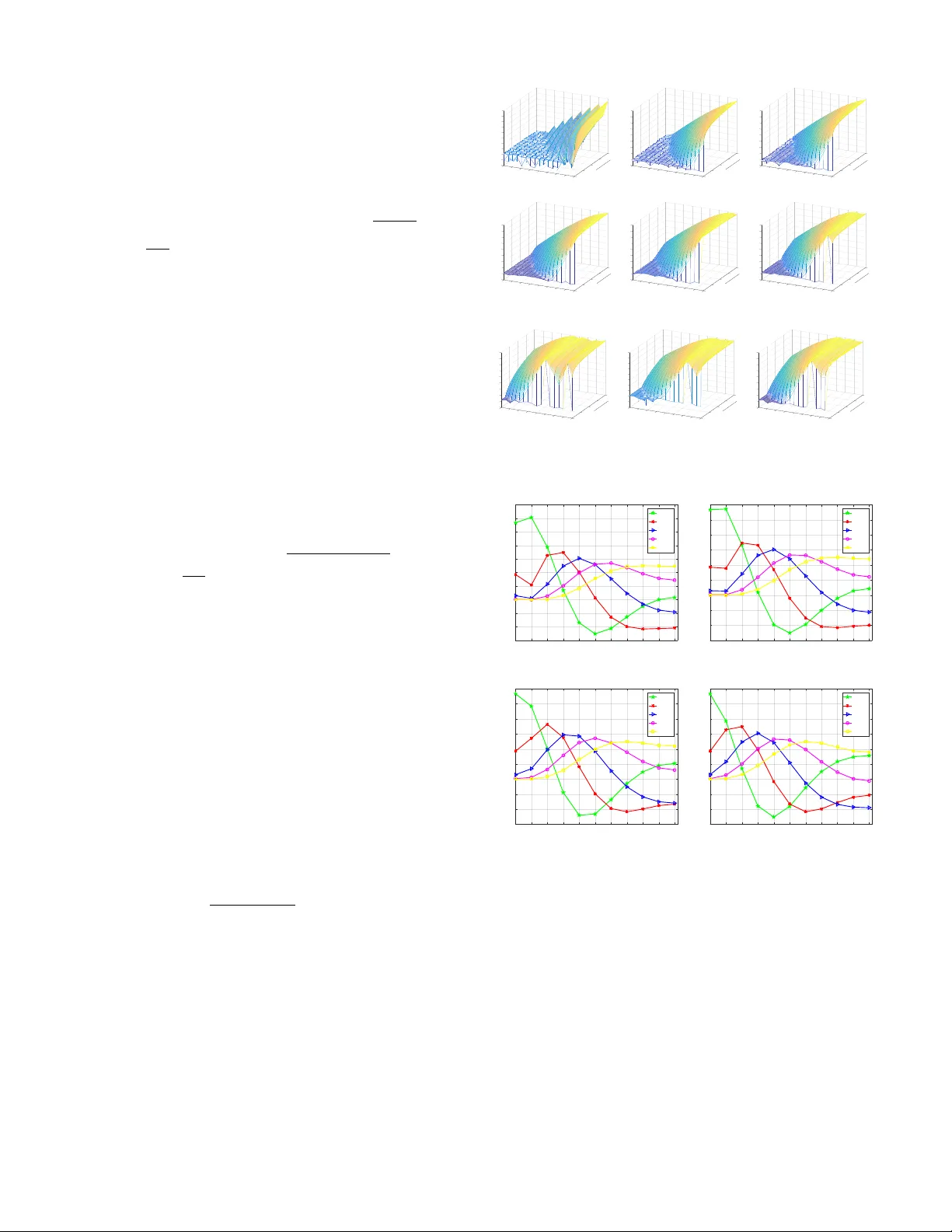
Radio V orte x W ireless Communications W ith Non-Coaxial UCA T ranscei v er Haiyue Jing and W enchi Cheng State K ey Laboratory of Integrated Services Netw orks, Xidian Uni versity , Xi’an, China E-mail: { hyjing@stu.xidian.edu.cn , wccheng@xidian.edu.cn } Abstract —In the past decade, more and mor e researchers ha ve concentrated on orbital-angular -momentum (O AM) based radio vortex wireless communications, which is expected to provide or - thogonality among different O AM-modes. The uniform circular array (UCA) is considered as one pr omising antenna structure for OAM based radio v ortex wir eless communications. However , most studies regarding UCA f ocus on the scenario where the transmit and recei ve UCAs are aligned with each other . In this paper , we in vestigate the radio vortex wir eless communications with non-coaxial UCA, i.e., the UCA transceivers are parallel b ut non-coaxial. W e study the channel model and de velop the mode- decomposition scheme to decompose the OAM-modes. Then, we discuss the impact of included angles on the channel model under non-coaxial scenario. Numerical results ar e presented to ev aluate our developed scheme and show that the spectrum efficiency of the non-coaxial UCA transceiver in some cases is larger than that of the aligned UCA transceiver based radio vortex wireless communications. Index T erms —Orbital angular momentum (O AM), uniform circular array (UCA), non-coaxial UCA, radio vortex wir eless communications. I . I N T RO D U C T I O N T HE plane w av e based wireless communications have becoming more and more matured, along with the well utilization of the traditional resources such as time and frequency [1]. T o further increase the spectrum ef ficiency , an ef ficient w ay is to explore other dimensional resources. During the past decade, orbital-angular-momentum (OAM), which is a kind of w av efront with helical phase front, has been attracted much attentions because dif ferent O AM-modes and the O AM-modes are orthogonal with each other [2]–[4]. Thus, using multiple OAM-modes for information transmission are expected to increase the spectrum ef ficiency for wireless communications. So far , many researches and experiments hav e been con- ducted to verify the feasibility of O AM based radio vortex wireless communications. The authors of [3] demonstrated a 32 Gbps millimeter-w ave link using four O AM-modes on each of two polarizations for data transmission. The authors of [5] experimentally demonstrated a 60 GHz wireless communications link using two O AM-modes. The authors of [6] theoretically and experimentally concluded that mode division multiple xing using O AM can reduce the receiver complexity and achieve high spectrum efficienc y . In addition, This work was supported in part by the National Natural Science F oun- dation of China (No. 61771368) and the Y oung Elite Scientists Sponsorship Program by CAST (2016QNRC001). the authors of [7], [8] held that OAM can be used in future wireless broadband communications because of its potential ability to achiev e high spectrum ef ficiency . Apart from the radio vorte x wireless communications, O AM based free-space optical communications has also been extensi vely studied [9], [10]. Specifically , uniform circular array (UCA) based OAM is considered as one promising antenna architecture for radio vorte x wireless communications because of its flexibility in transmitting multiple O AM beams with dif ferent O AM- modes [11], [12]. The schemes of O AM with index mod- ulation were proposed to achiev e much better error per- formance than the OAM based mode di vision multiplexing schemes [13]. The authors of [14] proposed a mode-hopping scheme within the narrow frequenc y band for anti-jamming in wireless communications, which can achie ve the same anti- jamming results as compared with the conv entional wideband frequency-hopping schemes. The authors of [15] proposed concentric UCAs system where the transmit and receive UCAs are aligned with each other to increase the spectrum efficienc y . For the UCA antenna structure, it is now highly demanded for strict alignment between the transmit and receiv e UCAs in current researches. Ho wev er , for wireless communications, it is not practical to maintain the transcei ver aligned with each other . If the transmit and receiv e UCAs are non-coaxial with each other , the phase of receiv ed signal contains not only the phase of O AM-mode, but also the phase turbulence due to unequal distance transmission at different places of the receiver [16], which challenges the efficient receiving for radio vortex wireless communications. Thus, a question is raised that how to decompose the O AM beams with multiple O AM-modes when the transmit and receive UCAs are non- coaxial. T o ov ercome the abov e-mentioned problem, in this paper we derive the mathematical model to characterize channel of non-coaxial radio vortex wireless communications. Based on the channel model, we develop the mode-decomposition scheme to obtain the signal corresponding to each OAM- mode. Also, the impact of concluded angles on the channel model is discussed. W e conduct extensi ve simulations to validate and e valuate that the spectrum ef ficiency of the non- coaxial UCA transceiver under some non-coaxial cases is larger than that of the aligned UCA transceiv er in radio vorte x wireless communications. The rest of this paper is org anized as follows. Section II   x y 2 N  r r  1 n N R  2 M  1 2 R M d mn d  d  x y z z Fig. 1. The system model for the non-coaxial UCA transceiv er based radio vorte x wireless communications. giv es the non-coaxial UCA transceiv er based radio vorte x wireless communications model. Section III in vestigates the channel model and dev elops the mode-decomposition scheme to obtain the receiv e signal corresponding to each OAM- mode. Section IV e valuates our dev eloped scheme and dis- cusses the channel amplitude gains versus the included an- gles under non-coaxial scenario. The paper concludes with Section V. I I . T H E N O N - C O A X I A L U C A S B A S E D S Y S T E M M O D E L F O R R A D I O V O RT E X W I R E L E S S C O M M U N I C AT I O N Figure 1 depicts the system model for the non-coaxial UCA transcei ver based radio v ortex wireless communications, where the transmit and recei ve UCAs are non-coaxial and the size of them can be different. The planes corresponding to the transmit and the recei ve UCAs are the transmit plane and the receive plane, respectiv ely . The projection of the transmit UCA is on the receiv e plane. W e denoted by d the distance from the center of the transmit UCA to the center of the receiv e UCA. The transmit and recei ve UCAs are equipped with N array-elements and M array-elements, respectiv ely . For the transmit UCA, the array-elements, which are fed with the same input signal but with a successi ve delay from array-element to array-element such that after a full turn the phase has been incremented by an integer multiple l of 2 π , are uniformly around the perimeter of the circle and l represents the number of topological char ges, i.e., the number of O AM-modes. For the receive UCA, the array- elements are also uniformly around perimeter of the circle. W e denote by α r and α R the angles between the phase angle of the first array-element and zero radian corresponding to the transmit and receive UCAs, respectiv ely . The parameter θ denotes the included angle between x -axis and the projection of the line from the center of the transmit UCA to the center of the recei ve UCA on the transmit plane. Also, φ denotes the included angle between z -axis and the line from the center of the transmit UCA to the center of the receiv e UCA. The notation e d represents the distance between the center of the transmit UCA and the center of the receiv e UCA. The parameter e d mn is the distance between the projection of the n th ( 1 ≤ n ≤ N ) transmit array-element on the receive plane and the m th ( 1 ≤ m ≤ M ) receiv e array-element. W e also denote by r the radius of transmit UCA and R the radius of receiv e UCA. In the follo wing, we deriv e the channel model and de velop the mode-decomposition scheme to obtain the signal corresponding to each O AM-mode. I I I . C H A N N E L M O D E L A N D T H E M O D E - D E C O M P O S I T I O N S C H E M E F O R N O N - C O A X I AL U C A S B A S E D R A D I O V O RT E X W I R E L E S S C O M M U N I C ATI O N S The signal at the n th array-element on the transmit UCA, denoted by x n , is gi ven as follows: x n = b N/ 2 c X l = b 2 − N 2 c 1 √ N s l e j ( ϕ n + α r ) l = b N/ 2 c X l = b 2 − N 2 c 1 √ N s l e j [ 2 π ( n − 1) N + α r ] l , (1) where ( ϕ n + α r ) is the azimuthal angle, defined as the angular position on a plane perpendicular to the axis of propagation, corresponding to the n th array-element on the transmit UCA. ϕ n = 2 π ( n − 1) / N is the basic angle for the transmit UCA. The symbol s l denotes the signal on the l th OAM-mode of the transmit UCA. l [ b (2 − N ) / 2 c ≤ l ≤ b N/ 2 c ] is the O AM- mode number . When κ < 0 , b κ c represents the smallest integer which is greater than or equal to κ . When κ ≥ 0 , b κ c represents the largest inte ger which is less than or equal to κ . W e denote by h mn the channel gain from the n th array- element on the transmit UCA to the m th array-element on the recei ve UCA. Then, h mn can be written as follows [17]: h mn = β λe − j 2 π λ d mn 4 π d mn , (2) where β denotes the combination of all the relev ant constants such as attenuation and phase rotation caused by antennas and their patterns on both sides. The parameter d mn is the distance between the n th array-element on the transmit UCA and the m th array-element on the receiv e UCA. W e denote by e d mn the distance between the projection of the n th array- element on the transmit UCA in the receiv e plane and the m th array-element on the recei ve UCA. Since the transmit UCA and the projection of transmit UCA are aligned well with each other , the distance e d mn should be deri ved first if we want to obtain d mn . In terms of rectangular coordinates, the coordinate of the n th array-element on the transmit UCA is ( r cos( ϕ n + α r ) , r sin( ϕ n + α r ) , 0) . The coordinate corresponding to the center of the receiv e UCA is ( d sin φ cos θ , d sin φ sin θ , d cos φ ) . Then, we have e d = d cos φ . Thus, the coordinate related to the projection e d mn = q [ R cos( ψ m + a R ) − d sin φ cos θ − r cos( ϕ n + α r )] 2 + [ R sin( ψ m + a R ) − d sin φ sin θ − r sin( ϕ n + α r )] 2 = q R 2 + r 2 + d 2 sin 2 φ − 2 r R cos( ψ m + a R − ϕ n − α r ) − 2 Rd sin φ cos( ψ m + a R − θ ) + 2 r d sin φ cos( ϕ n + α r − θ ) . (3) d mn = q e d 2 mn + e d 2 = p R 2 + r 2 + d 2 − 2 r R cos( ψ m + a R − ϕ n − α r ) − 2 Rd sin φ cos( ψ m + a R − θ ) + 2 rd sin φ cos( ϕ n + α r − θ ) = p R 2 + r 2 + d 2 r 1 − 2 r R cos( ψ m + a R − ϕ n − α r ) + 2 Rd sin φ cos( ψ m + a R − θ ) − 2 rd sin φ cos( ϕ n + α r − θ ) R 2 + r 2 + d 2 ≈ p R 2 + r 2 + d 2 − r R cos( ψ m + a R − ϕ n − α r ) + Rd sin φ cos( ψ m + a R − θ ) − rd sin φ cos( ϕ n + α r − θ ) √ R 2 + r 2 + d 2 . (4) h mn = β λ 4 π √ d 2 + r 2 + R 2 exp − j 2 π √ d 2 + r 2 + R 2 λ ! exp  j 2 π Rd sin φ cos( ψ m + a R − θ ) λ √ d 2 + r 2 + R 2  | {z } A m × exp      − j 2 π r q R 2 + d 2 sin 2 φ − 2 Rd sin φ cos( ψ m + a R − θ ) λ √ d 2 + r 2 + R 2 | {z } B m sin( ϕ n + α r − ψ m − a R + ζ m )      . (7) of the n th array-element on the transmit UCA in the recei ve plane is ( r cos( ϕ n + α r ) , r sin( ϕ n + α r ) , d cos φ ) and the coordinate of the m th array-element on the receiv e UCA is ( R cos( ψ m + a R ) − d sin φ cos θ, R sin( ψ m + a R ) − d sin φ sin θ , d cos φ ) . Similar to the azimuthal angle at the transmit UCA, ψ m + a R is the azimuthal angle of the m th array-element on the receiv e UCA and ψ m = 2 π ( m − 1) / M is the basic angle for the receiv e UCA. Therefore, e d mn is deriv ed in Eq. (3). Then, using the Pythagorean theorem we can deri ved d mn in Eq. (4). Because d  R and d  r , we hav e d mn ≈ √ d 2 + R 2 + r 2 for the denominator in Eq. (2). For d mn in the numerator, which is part of the item exp ( − j 2 π d mn /λ ) , we can approximate it using √ 1 − 2 x ≈ 1 − x when x is very close to zero as sho wn in Eq. (4). In Eq. (4), the item  2 r R cos( ψ m + a R − ϕ n − α r ) − 2 r d sin φ cos( ϕ n + α r − θ )  can be deri ved as follows: r R cos( ψ m + a R − ϕ n − α r ) − r d sin φ cos( ϕ n + α r − θ ) = [ Rr − rd sin φ cos( ψ m + a R − θ )] cos( ϕ n + α r − ψ m − a R ) + r d sin φ sin( ψ m + a R − θ ) sin( ϕ n + α r − ψ m − a R ) = r q R 2 + d 2 sin 2 φ − 2 Rd sin φ cos( ψ m + a R − θ ) × sin( ϕ n + α r − ψ m − a R + ζ m ) , (5) where      sin ζ m = R − d sin φ cos( ψ m + a R − θ ) √ R 2 + d 2 sin 2 φ − 2 Rd sin φ cos( ψ m + a R − θ ) ; cos ζ m = d sin φ sin( ψ m + a R − θ ) √ R 2 + d 2 sin 2 φ − 2 Rd sin φ cos( ψ m + a R − θ ) . (6) Associating Eqs. (2), (4), (5), and (6), the channel gain h mn can be deri ved as Eq. (7). F or conv enient expression, we replace some polynomials in Eq. (7) with A m and B m , respectiv ely , as shown in Eq. (7). The recei ved signal at the m th array-element, denoted by y m , can be deri ved as follows: y m = N X n =1 b N/ 2 c X l = b 2 − N 2 c h mn 1 √ N s l e j 2 π ( n − 1) N l + z m = b N/ 2 c X l = b 2 − N 2 c e h ml s l + z m , (8) where z m denotes the recei ved noise at the m th array-element on the receiv e UCA and z m is comple x Gaussian v ariable with zero mean and variance σ 2 m . W e denote by e h ml the channel gain from the transmit UCA to the m th array-element on the receive UCA corresponding to the l th O AM-mode. The channel gain e h ml is giv en by Eq. (9). In Eq. (9), ϕ is the continuous variable related to ϕ n ranging from 0 and 2 π . When n is equal to 1, ϕ n is equal to zero. When n = N , ϕ n is equal to 2 π − 2 π / N and very close to 2 π . T o express con veniently , we denote by ψ = α r − ψ m − a R + ζ m , which is used in Eq. (9). e h ml = N X n =1 1 √ N h mn e j 2 π ( n − 1) N l = N X n =1 A m √ N exp [ − B m sin( ϕ n + α r − ψ m − a R + ζ m )] exp [ j ( ϕ n + α r ) l ] = A m √ N exp [ j ( ψ m + a R − ζ m ) l ] N X n =1 exp [ j ( ϕ n + α r − ψ m − a R + ζ m ) l ] exp [ − B m sin( ϕ n + α r − ψ m − a R + ζ m )] ≈ √ N A m exp [ j ( ψ m + a R − ζ m ) l ] 1 2 π Z 2 π 0 exp[ j ( ϕ + α r − ψ m − a R + ζ m | {z } ψ ) l ] exp [ − B m sin( ϕ + α r − ψ m − a R + ζ m )] dϕ = √ N A m exp [ j ( ψ m + a R − ζ m ) l ] 1 2 π Z 2 π + ψ ψ exp [ j ( ϕ + ψ ) l ] exp [ − B m sin( ϕ + ψ )] d ( ϕ + ψ ) = √ N A m exp [ j ( ψ m + a R − ζ m ) l ] 1 2 π Z 2 π 0 exp [ j ( ϕ + ψ ) l ] exp [ − B m sin( ϕ + ψ )] d ( ϕ + ψ ) = √ N A m exp [ j ( ψ m + a R − ζ m ) l ] J l ( B m ) = √ N β λ 4 π √ d 2 + r 2 + R 2 exp − j 2 π √ d 2 + r 2 + R 2 λ ! | {z } h exp [ j ( ψ m + a R − ζ m ) l ] × exp  j 2 π Rd sin φ cos( ψ m + a R − θ ) λ √ d 2 + r 2 + R 2  J l   2 π r q R 2 + d 2 sin 2 φ − 2 Rd sin φ cos( ψ m + a R − θ ) λ √ d 2 + r 2 + R 2   | {z } C m,l . (9) In Eq. (9), the l -order Bessel function is gi ven as follows: J l ( α ) = 1 2 π Z 2 π 0 e j lτ e − j α sin τ dτ . (10) Observing Eq. (10), we can find that e j lτ e − j α sin τ is the function, of which τ is the independent variable, with period 2 π when l is an integer . This is the reason why the line 4 of Eq. (7) is equal to the line 5 of Eq. (7). Also, we replace some polynomials in Eq. (7) with h and C m,l , respectively , as shown in Eq. (7) for con venient expression. In the following, we show two cases corresponding to dif ferent included angles θ and φ as follows: Case A: When φ is equal to zero, the transmit and receive UCAs are are coaxial and parallel to each other . In this case, the channel gain e h ml can be re written as follo ws: e h ml = hJ l  2 π rR λ √ d 2 + r 2 + R 2  e j ( ψ m + a R − π 2 ) l . (11) W e can find that the channel amplitude gain | e h ml | only depends on the order of OAM-mode and ψ m is independent on | e h ml | when r , R , λ , and N are fixed. Thus, we can consider that the signals carried by different O AM-modes correspond to dif ferent channel amplitude gains. Case B: When φ is equal to π / 2 , the transmit and receiv e UCAs are both on the transmit plane. In this case, we denote by θ = α R and we ha ve      B m = 2 π r √ R 2 + d 2 − 2 Rd cos ψ m λ √ d 2 + r 2 + R 2 ; C m,l = exp  j 2 πRd cos ψ m λ √ d 2 + r 2 + R 2  J l ( B m ) . (12) Thus, the channel amplitude gain | e h ml | depends on ψ m apart from the order of O AM-mode. The error , denoted by e l , corresponding to the l th O AM- mode for the approximation in Eq. (9) is deri ved as follows: e l = log 10 " hC m,l e j ( ψ m + a R − ζ m ) l − N X n =1 1 √ N h mn e j ϕ n l # . (13) Then, based on Eq. (9), we can rewrite y m as follo ws: y m = b N/ 2 c X l = b 2 − N 2 c e h ml s l = b N/ 2 c X l = b 2 − N 2 c hC m,l s l e j [ 2 π ( m − 1) M + a R − ζ m ] l + z m , (14) T o recover the transmit signal corresponding to the l 0 th ( b (2 − N ) / 2 c ≤ l 0 ≤ b N / 2 c ) O AM-mode, the receiv ed signal y m is multiplied with the item C − 1 m,l 0 exp[ − j ( ψ m + a R − ζ m ) l 0 ] . Then, we denote by y m,l 0 the recei ved signal related to l 0 at the m th array-element on the receiv e UCA and y m,l 0 can be written as follo ws: y m,l 0 = y m C − 1 m,l 0 e − j [ 2 π ( m − 1) M + a R − ζ m ] l = b N/ 2 c X l = b 2 − N 2 c hs l e j ( a R − ζ m )( l − l 0 ) e j 2 π ( m − 1) M ( l − l 0 ) + z m C − 1 m,l 0 e − j ( ψ m + a R − ζ m ) l 0 . (15) Therefore, the receiv ed signal, denoted by y l 0 , corresponding to the l 0 th O AM-mode of the receiv e UCA can be deriv ed as follows: y l 0 = M X m =1 y m,l 0 = b N/ 2 c X l = b 2 − N 2 c ,l 6 = l 0 hs l e j ( a R − ζ m )( l − l 0 ) M X m =1 e j 2 π ( m − 1) M ( l − l 0 ) + M X m =1 hs l 0 + M X m =1 z m C − 1 m,l 0 e − j ( ψ m + a R − ζ m ) l 0 = M hs l 0 + M X m =1 z m C − 1 m,l 0 e − j ( ψ m + a R − ζ m ) l 0 . (16) T rav ersing the O AM-mode l 0 , we can obtain all the esti- mated transmit signals. Because z m is the complex Gaussian variable with zero mean and variance σ 2 m , we can deriv e that P M m =1 z m C − 1 m,l 0 e − j ( ψ m + a R − ζ m ) l 0 is a complex Gaussian variable with zero mean and variance P M m =1 C − 2 m,l 0 σ 2 m . Then, the spectrum ef ficiency , denoted by C OAM , for the radio vorte x wireless communications under the non-coaxial UCA transceiv er scenario can be deriv ed as follo ws: C OAM = b N/ 2 c X l = b 2 − N 2 c log 2 1 + M 2 h 2 | s l | 2 P M m =1 C − 2 m,l 0 σ 2 m ! . (17) I V . P E R F O R M A N C E E V A L UAT I O N S In this section, we ev aluate the performance of non-coaxial UCA transcei ver based radio v ortex wireless communications. First, we e valuate the approximation error corresponding to dif ferent O AM-modes. Then, we e valuate the channel amplitude gains for different O AM-modes versus the included angle θ and φ , respectiv ely . Figure 2 sho ws the approximation error of different OAM- modes for the non-coaxial UCA transceiver scenario, where we set β = 4 π , α r = α R = 0 , θ = φ = 0 , and λ = 0 . 1 m. W e can observe that when the number of array-elements is larger than 10, the corresponding error is very small and can be ignored. Therefore, e h ml is relatively very accurate when the number of array-elements is larger than 10. Also, the error mainly depends on the number of array-elements while the value of 2 π rR /  λ √ d 2 + r 2 + R 2  has small impact on the error for dif ferent O AM-modes. Figure 3 displays the values of | e h ml | for dif ferent OAM- modes with respect to φ , where we set β = 4 π , N = M = 10 , λ = 0 . 1 m, r = R = λ , d = 10 λ , α r = α R = 0 , and θ = 0 . As shown in Fig. 3, the channel amplitude gain corresponding to O AM-mode 0 first decreases and then increases as the included angle φ increases. While the channel amplitude gains corresponding to other O AM-modes first increase and then decrease as the included angle φ increases. The channel amplitude gains corresponding to different basic angle ψ m are almost the same. Figure 4 depicts the v alues of | e h ml | for dif ferent O AM- modes with respect to θ , where we set β = 4 π , N = M = 10 , 2 : rR= ! 6 p d 2 + r 2 + R 2 " The number of array-elements 2 1.5 -20 1 -18 20 -16 18 -14 16 -12 0.5 -10 14 e 0 -8 12 -6 10 -4 8 -2 6 0 0 4 l = 0 2 : rR= ! 6 p d 2 + r 2 + R 2 " The number of array-elements 2 1.5 -18 1 -16 20 -14 18 -12 16 -10 0.5 14 e 1 -8 12 -6 10 -4 8 -2 6 0 0 4 l = 1 The number of array-elements 2 : rR= ! 6 p d 2 + r 2 + R 2 " e 2 2 1.5 -18 1 -16 20 -14 18 -12 16 -10 0.5 14 -8 12 -6 10 -4 8 -2 6 0 0 4 l = 2 The number of array-elements 2 : rR= ! 6 p d 2 + r 2 + R 2 " 2 1.5 -18 1 -16 20 -14 18 -12 16 -10 0.5 14 e 3 -8 12 -6 10 -4 8 -2 6 0 0 4 l = 3 2 : rR= ! 6 p d 2 + r 2 + R 2 " The number of array-elements e 4 2 1.5 -18 1 -16 20 -14 18 -12 16 -10 0.5 14 -8 12 -6 10 -4 8 -2 6 0 0 4 l = 4 The number of array-elements 2 : rR= ! 6 p d 2 + r 2 + R 2 " 2 1.5 -18 1 -16 20 -14 18 -12 16 -10 0.5 14 e 5 -8 12 -6 10 -4 8 -2 6 0 0 4 l = 5 2 : rR= ! 6 p d 2 + r 2 + R 2 " The number of array-elements 2 1.5 -18 1 -16 20 -14 18 -12 16 -10 0.5 14 e 6 -8 12 -6 10 -4 8 -2 6 0 0 4 l = 6 2 : rR= ! 6 p d 2 + r 2 + R 2 " The number of array-elements e 7 2 1.5 -20 1 -18 20 -16 18 -14 16 -12 0.5 -10 14 -8 12 -6 10 -4 8 -2 6 0 0 4 l = 7 2 : rR= ! 6 p d 2 + r 2 + R 2 " The number of array-elements 2 1.5 -18 1 -16 20 -14 18 -12 16 -10 0.5 14 e 8 -8 12 -6 10 -4 8 -2 6 0 0 4 l = 8 Fig. 2. Approximation error from OAM-mode 0 to OAM-mode 8. 0 : /20 2 : /20 3 : /20 4 : /20 5 : /20 6 : /20 7 : /20 8 : /20 9 : /20 : /2 ? -0.15 -0.1 -0.05 0 0.05 0.1 0.15 0.2 0.25 0.3 0.35 - - - e h 1 l - - - l = 0 l = 1 l = 2 l = 3 l = 4 m = 1 0 : /20 2 : /20 3 : /20 4 : /20 5 : /20 6 : /20 7 : /20 8 : /20 9 : /20 : /2 ? -0.15 -0.1 -0.05 0 0.05 0.1 0.15 0.2 0.25 0.3 - - - e h 2 l - - - l = 0 l = 1 l = 2 l = 3 l = 4 m = 2 0 : /20 2 : /20 3 : /20 4 : /20 5 : /20 6 : /20 7 : /20 8 : /20 9 : /20 : /2 ? -0.15 -0.1 -0.05 0 0.05 0.1 0.15 0.2 0.25 0.3 - - - e h 3 l - - - l = 0 l = 1 l = 2 l = 3 l = 4 m = 3 0 : /20 2 : /20 3 : /20 4 : /20 5 : /20 6 : /20 7 : /20 8 : /20 9 : /20 : /2 ? -0.15 -0.1 -0.05 0 0.05 0.1 0.15 0.2 0.25 0.3 - - - e h 4 l - - - l = 0 l = 1 l = 2 l = 3 l = 4 m = 4 Fig. 3. | e h ml | for different OAM-modes with different m . λ = 0 . 1 m, r = R = λ , d = 10 λ , α r = α R = 0 , and φ = π/ 3 . For different ψ m , the channel amplitude gains randomly change. Also, the dynamic range of channel amplitude gains for all the O AM-modes is small as the included angle θ increases. Figure 5 sho ws the spectrum efficiency versus the included angle φ , where we set β = 4 π , N = M = 10 , λ = 0 . 1 m, r = R = λ , d = 10 λ , α r = α R = 0 , and θ = 0 . W e can observe that the maximum spectrum ef ficiency is achiev ed when the included angle φ is approximately equal to 2 π / 5 . In some cases, the spectrum efficiency of the non-coaxial UCA transceiv er is larger than that of the aligned UCA transcei ver based radio vortex wireless communications. That is to say , 0 : /20 2 : /20 3 : /20 4 : /20 5 : /20 6 : /20 7 : /20 8 : /20 9 : /20 : /2 3 -0.15 -0.1 -0.05 0 0.05 0.1 0.15 - - - e h 1 l - - - l = 0 l = 1 l = 2 l = 3 l = 4 m = 1 0 : /20 2 : /20 3 : /20 4 : /20 5 : /20 6 : /20 7 : /20 8 : /20 9 : /20 : /2 3 -0.15 -0.1 -0.05 0 0.05 0.1 0.15 - - - e h 2 l - - - l = 0 l = 1 l = 2 l = 3 l = 4 m = 2 0 : /20 2 : /20 3 : /20 4 : /20 5 : /20 6 : /20 7 : /20 8 : /20 9 : /20 : /2 3 -0.15 -0.1 -0.05 0 0.05 0.1 0.15 - - - e h 3 l - - - l = 0 l = 1 l = 2 l = 3 l = 4 m = 3 0 : /20 2 : /20 3 : /20 4 : /20 5 : /20 6 : /20 7 : /20 8 : /20 9 : /20 : /2 3 -0.15 -0.1 -0.05 0 0.05 0.1 0.15 - - - e h 4 l - - - l = 0 l = 1 l = 2 l = 3 l = 4 m = 4 Fig. 4. | e h ml | for different OAM-modes with different m . 0 : /20 2 : /20 3 : /20 4 : /20 5 : /20 6 : /20 7 : /20 8 : /20 9 : /20 : /2 ? 2.5 2.6 2.7 2.8 2.9 3 3.1 Spectrum efficiency (bps/Hz) Fig. 5. The spectrum efficiency versus the included angle φ . the scenario where the transmit and recei ve UCAs are aligned with each other is not the best scene to achieve the spectrum efficienc y maximization. V . C O N C L U S I O N S W e in vestigated the non-coaxial scenario where the transmit and recei ve UCAs are non-coaxial with each other . Then, we deri ved the channel model and de veloped the mode- decomposition scheme to obtain the transmit signal corre- sponding to each OAM-mode. Then, we discussed the impact of included angles θ and φ on the channel gains. The simulation results v alidated that in some cases the spectrum efficienc y of the non-coaxial UCA transceiver is larger than that of the aligned UCA transceiv er based radio vorte x wireless communications. R E F E R E N C E S [1] J. G. Andrews, S. Buzzi, W . Choi, S. V . Hanly , A. Lozano, A. C. K. Soong, and J. C. Zhang, “What will 5G be? ” IEEE Journal on Selected Ar eas in Communications , vol. 32, no. 6, pp. 1065–1082, June 2014. [2] F . T amburini, E. Mari, A. Sponselli, F . Romanato, B. Thid ´ e, A. Bian- chini, L. Palmieri, and C. G. Someda, “Encoding many channels in the same frequency through radio vorticity: first experimental test, ” New Journal of Physics , vol. 14, no. 3, 2013. [3] Y . Y an, G. Xie, M. P . J. Lav ery , H. Huang, N. Ahmed, C. Bao, Y . Ren, Y . Cao, L. Li, and Z. Zhao, “High-capacity millimetre-wav e communications with orbital angular momentum multiplexing, ” Nature Communications , vol. 5, 2014. [4] K. A. Opare, Y . Kuang, J. J. Kponyo, K. S. Nwizege, and Z. Enzhan, “The degrees of freedom in wireless line-of-sight O AM multiplexing systems using a circular array of receiving antennas, ” in F ifth Interna- tional Conference on Advanced Computing Communication T echnolo- gies , 2015, pp. 608–613. [5] Z. Zhao, Y . Y an, L. Li, G. Xie, Y . Ren, N. Ahmed, Z. W ang, C. Liu, A. J. W illner , P . Song, H. Hashemi, H. Y ao, D. Macfarlane, R. Henderson, N. Ashrafi, S. Ashrafi, S. T alwar , S. Sajuyigbe, M. T ur , A. F . Molisch, and A. E. W illner, “ A dual-channel 60 GHz communications link using patch antenna arrays to generate data-carrying orbital-angular- momentum beams, ” in 2016 IEEE International Confer ence on Com- munications (ICC) , May 2016, pp. 1–6. [6] W . Zhang, S. Zheng, X. Hui, R. Dong, X. Jin, H. Chi, and X. Zhang, “Mode division multiplexing communication using microw ave orbital angular momentum: An experimental study , ” IEEE T ransactions on W ireless Communications , vol. 16, no. 2, pp. 1308–1318, Feb . 2017. [7] X. Ge, R. Zi, X. Xiong, Q. Li, and L. W ang, “Millimeter wa ve communications with OAM-SM scheme for future mobile networks, ” IEEE Journal on Selected Ar eas in Communications , vol. PP , no. 99, pp. 1–1, 2017. [8] Q. Zhu, T . Jiang, Y . Cao, K. Luo, and N. Zhou, “Radio vortex for future wireless broadband communications with high capacity , ” IEEE W ireless Communications , vol. 22, no. 6, pp. 98–104, Dec. 2015. [9] M. Cheng, L. Guo, J. Li, and Y . Zhang, “Channel capacity of the O AM-based free-space optical communication links with bessel-Gauss beams in turbulent ocean, ” IEEE Photonics Journal , vol. 8, no. 1, pp. 1–11, Feb . 2016. [10] A. E. Willner , “Communication with a twist, ” IEEE Spectrum , vol. 53, no. 8, pp. 34–39, Aug. 2016. [11] S. M. Mohammadi, L. K. S. Daldorff, J. E. S. Bergman, R. L. Karlsson, B. Thid ´ e, K. Forozesh, T . D. Carozzi, and B. Isham, “Orbital angular momentum in radio-a system study , ” IEEE T ransactions on Antennas and Pr opagation , v ol. 58, no. 2, pp. 565–572, Feb . 2010. [12] Q. Bai, A. T ennant, and B. Allen, “Experimental circular phased array for generating OAM radio beams, ” Electronics Letters , vol. 50, no. 20, pp. 1414–1415, Sep. 2014. [13] E. Basar , “Orbital angular momentum with index modulation, ” IEEE T ransactions on W ir eless Communications , vol. 17, no. 3, pp. 2029– 2037, Mar . 2018. [14] L. Liang, W . Cheng, W . Zhang, and H. Zhang, “Mode hopping for anti-jamming in radio v ortex wireless communications, ” to appear in IEEE T ransactions on V ehicular T echnology , pp. 1–15, 2018. [15] H. Jing, W . Cheng, Z. Li, and H. Zhang, “Concentric UCAs based low- order radio vortex wireless communications with co-mode interference (in vited paper), ” in 2017 IEEE/CIC International Confer ence on Communications in China (ICCC) , Oct. 2017, pp. 1–6. [16] W . Cheng, W . Zhang, H. Jing, S. Gao, and H. Zhang, “Orbital angular momentum for wireless communications, ” to appear in IEEE W ir eless Communications Magazine , pp. 1–15, 2018. [17] O. Edfors and A. J. Johansson, “Is orbital angular momentum (O AM) based radio communication an unexploited area?, ” IEEE Tr ansactions on Antennas and Pr opagation , vol. 60, no. 2, pp. 1126–1131, 2012.