Learning to Transcribe by Ear

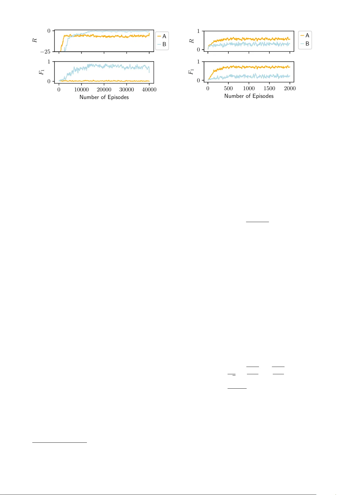
LEARNING T O TRANSCRIBE BY EAR Rainer K elz, Gerhard W idmer Institute of Computational Perception Johannes K epler Uni v ersity Linz, Austria rainer.kelz@jku.at ABSTRA CT Rethinking how to model polyphonic transcription for- mally , we frame it as a reinforcement learning task. Such a task formulation encompasses the notion of a musical agent and an en vironment containing an instrument as well as the sound source to be transcribed. W ithin this concep- tual framew ork, the transcription process can be described as the agent interacting with the instrument in the en viron- ment, and obtaining rew ard by playing along with what it hears. Choosing from a discrete set of actions - the notes to play on its instrument - the amount of re ward the agent ex- periences depends on which notes it plays and when. This process resembles ho w a human musician might approach the task of transcription, and the satisfaction she achiev es by closely mimicking the sound source to transcribe on her instrument. Follo wing a discussion of the theoretical framework and the benefits of modelling the problem in this way , we fo- cus our attention on sev eral practical considerations and address the difficulties in training an agent to acceptable performance on a set of tasks with increasing difficulty . W e demonstrate promising results in partially constrained en vironments. 1. INTR ODUCTION Polyphonic transcription is the task of extracting a set of symbolic notes from audio. T ypical transcription sys- tems, as e xemplified by [1, 3, 4, 7, 10] w ork on spectro- gram frames and output a note activity vector for each frame. These note acti vity vectors are the input to a tem- poral smoothing, thresholding and decoding stage, finally leading to the construction of note objects. A note object, or symbolic note, can be described as a tuple ( t s , t e , p, v ) comprised of a start point (onset) and end point (offset) in time, a symbolic pitch p , directly related to the fundamen- tal frequency of the sound. Optionally , a note object might indirectly encode the volume of the note via the so called velocity v . Solving a polyphonic transcription task therefore en- compasses explaining a dense mixture of v arious sounds ov er time in terms of comparatively fewer and temporally c  Rainer K elz, Gerhard W idmer. Licensed under a Cre- ativ e Commons Attribution 4.0 International License (CC BY 4.0). At- tribution: Rainer Kelz, Gerhard W idmer . “LEARNING TO TRAN- SCRIBE BY EAR”, A GENT ENVIRONMENT PER CEIVE A CT Figure 1 : Sketch of the agent-environment interaction loop much sparser distributed causes, such as the discrete deci- sion to press a k ey on a musical ke yboard, or pluck a string at a particular point in time, as well as choosing when to lift the finger from the key , or muting the string again. All of the above mentioned transcription systems obtain approximate solutions to the problem by solving a contin- uous optimization problem. The continuous optimization problem usually arises by introducing smooth relaxations. Discrete step functions are replaced by smooth nonlinear- ities, such as the tanh function or scaled versions thereof. Discrete performance measures, such as accuracy or pre- cision, recall and f-measure are replaced by surrogate loss functions such as mean squared error or binary cross en- tropy . This necessitates having either fixed thresholds to obtain discrete decisions after training, or tuning thresh- olds on holdout data. Instead of optimizing surrogate losses we opt to directly model the discrete decision making process of playing in- dividual notes in a musical piece, together with the conse- quences of these individual decisions. W e choose to model the polyphonic transcription task in a way that is reminiscent of a human listening to audio, trying to recreate what she hears by playing along on her instrument. The better the recreation produced by a mu- sical agent, be it human or machine, the more rewarding the experience. In [6] an informal study on how musicians transcribe audio recordings was undertaken. The authors report that many people describe their approach roughly as [...] build up a mental representation, and then play this on an instrument, sometimes along with the original audio. [...] A sketch of the interaction model can be seen in Figure 1. There are tw o main entities, the agent and the en- vironment that the agent interacts with. The musical agent perceiv es the state of the en vironment, which is comprised of a few spectrogram frames of the sound source that the agent wants to reproduce, and the current state of the in- strument on which to reproduce the piece. The state of the instrument is discrete and reflects which notes are sound- ing currently . The reward of the agent is given by the environment and reflects the acoustic similarity between what is heard from the sound source and what is currently being played on the instrument. If what is being played is identical to what should be reproduced, the rew ard is maximal. In section 2 we will introduce the necessary formalisms to model the transcription problem and solve it via rein- forcement learning methods, section 3 will introduce ac- tual solution methods, in section 4 we will describe key aspects of the en vironment, and in section 5 we will dis- cuss results from computational experiments. 2. MARK OV DECISION PR OCESSES W e will now formally define Markov decision processes, and then cast the transcription problem as such a process. This section as a whole relies heavily on [11], chapters 1-3. W e also adhere to the notational style of [11], where upper - case letters refer to random variables and lo wercase letters to their realizations. A Markov decision process (MDP) is a collection of random variables ordered in time. Time is assumed to be discrete, and subscripts index the time dimension. An MDP is described by a tuple ( S , A , R , T , γ ) consisting of a state space S , a set of possible actions A ( s ) to take in a particular state s , a scalar re ward function R that de- termines how much immediate rew ard is gained from be- ing in a particular state s at a particular point in time t , and a stochastic state transition function T in the form of a conditional probability distribution over successor states p ( s 0 | s, a ) , conditioned on the current state and a particular action. This distribution has the Markov property , meaning that the following equality holds: p ( S t | S t − 1 , A t − 1 ) = p ( S t | S t − 1 , A t − 1 , . . . S 0 , A 0 ) The e volution of a Markov decision process over time starts with a random state S 0 . The agent percei ves the state, and decides on an action A 0 . The environment reacts to the action A 0 and determines its consequences - the successor state S 1 and a re ward R 1 - whereupon the c ycle begins anew . This leads to trajectories through state space: S 0 , A 0 , R 1 , S 1 , A 1 , R 2 , S 2 , A 2 . . . If these trajectories have a natural end, they are also re- ferred to as episodes. The behavior of the agent is governed by the policy π ( a | s ) . The polic y is a probability distrib ution ov er ac- tions, conditioned on the state s . The only goal of an agent is to beha ve in such a way as to maximize the expected fu- ture reward v π ( s ) = E [ G t | S t = s ] , from the current state onwards. The function v π ( s ) is called the state value func- tion. It is defined in terms of the return G t , which is the sum of all future reward discounted by the factor γ ∈ [0 , 1] G t = ∞ X k =0 γ k R t + k +1 (a) Interaction loop (b) The definition of a state Figure 2 : Illustration of the agent-en vironment interaction loop, and how states, re ward and actions look like How much v alue a state gets assigned, depends on the behavior , the policy π . An agent has to learn a policy by interaction with the en vironment such that the expected fu- ture reward v π ( · ) is maximized. W e will now discuss mod- elling polyphonic transcription as an MDP in greater detail. 2.1 T ranscription as an MDP As mentioned in the introduction, we model transcription as the interaction of a musical agent with an en vironment. The agent perceiv es music from an ambient sound source, and plays along on its instrument. The closer the instru- mental reproduction, the more rew ard is experienced. T ime is assumed to be discrete, subscripts index timesteps. Interaction is strictly formalized such that the only inputs the agent has at its disposal are the current state S t and the current rew ard R t , and the only way for the agent to interact with the en vironment is to decide on the current action A t , as is illustrated in Figure 2a. Af- ter time advances by one step, the agent percei ves the next state S t +1 as well as the next re ward R t +1 . The main modelling effort lies in specifying what a state looks like, how the environment reacts to an action by transitioning to a new state and how it assigns rew ard. Although we in vestigated multiple versions of the en vi- ronment with slight differences in how the state was con- structed, we describe only a prototypical version here. Ex- act specifications of environments, agents and models to reproduce all findings are av ailable as source code on- line 1 . W e define the state as a tuple s = ( X t , ∆ X t , k ) . The vector x t describes the current spectrogram frame for the sound source that should be transcribed. The matrix X t = [ x t − c , . . . , x t , . . . , x t + c ] consists of the last c spec- trogram frames, the current frame at time t and c future frames. The overall lag of the system with respect to the sound source to be transcribed is therefore exactly c frames. Additionally , ∆ X t encodes the finite difference in time direction as a low level feature sensitive to onsets. This is redundant, as this information is already contained in X t , b ut facilitates learning for the class of models under consideration in section 5. k is a binary indicator vector encoding the current state of the virtual musical keyboard of the instrument. If the k th key is pressed, meaning that the k th note is currently sounding, the k th component of this vector is set to 1 , otherwise it is 0 . The en vironment knows the exact, discrete current state of the instrument because of the agent’ s previous actions leading up to this state, namely which keys have been pressed and released again. 1 http://available.upon.publicat.ion The reward R t at each timestep is what implicitly de- fines the goal of a reinforcement learning task. It should be high if a state is desirable, and low in undesirable states. For the case of transcription, any measure appears to be reasonable that measures the similarity between the sound to be transcribed, and the sound produced by the agent’ s virtual instrument. W e in vestigate multiple audio similar- ity measures, but defer discussion of their differences and resulting differences in agent beha vior until section 5. The MDP formalism allows for the agent to decide on exactly one action A t in each timestep. This w ould e x- clude polyphonic instruments. T o allow for polyphon y , we define the actions A ( s ) av ailable in a state as playing all possible note combinations from the set of playable notes. If the tonal range of the instrument is K , the number of all possible note combinations is 2 K . This would lead to an unnecessarily large number of outputs for the model. W e therefore output a binary indicator vector with K compo- nents that index es into the set of possible actions. 2.2 Benefits W e are con vinced that this way of looking at the problem has merit. After its formal introduction we would like to emphasize some of the benefits of the MDP perspectiv e on transcription. T o summarize the previous section, the agent perceiv es a short spectrogram snippet (the matrix X t ) and a low-le vel onset feature (the matrix ∆ X t ) of the sound source it is supposed to transcribe, as well as the state of the musical keyboard of the virtual instrument it is play- ing by way of an indicator vector (the vector k ) that tells the agent which keys are currently pressed. The action an agent chooses at each time step is in the form of a binary vector as well, indicating whether to press a key or stop pressing it. This perspectiv e on the problem of transcription has multiple benefits. Labelled data becomes unnecessary to learn a transcription model. Supervision is replaced by in- teraction with a computer controllable instrument, such as a software sampler, a physical simulation of an instrument, or ev en an actual automatic reproducing piano, such as a Disklavier . Anything that is controllable by MIDI mes- sages can be used to learn to transcribe unlabelled data. A second benefit, closely tied in with the first, is that the temporal e volution of notes is modelled implicitly . The agent can only start and stop a note, there is no leeway in the decision making process to modify the note intermedi- ately in any way . Hence there is also no need to try and explicitly force this behavior , for example via a constraint to a continuous optimization problem, as done in [4]. A third benefit is that in order to transcribe ne w , unseen material, the agent simple needs to be set loose and allowed to maximize re ward. Depending on how much music it has listened to in the past, it will start from an already reason- able solution, that is then iteratively refined. As an added bonus, we obtain a better, more general recognition model during this procedure, which can then be applied to the next piece - the model improves continuously with each application. 3. POLICY GRADIENT METHODS W e will no w discuss a particular solution method for MDPs that directly learns a policy π . This discussion relies heavily on [11], chapter 13. Readers not familiar with (or not interested in) the de- tails of reinforcement learning may decide to skip this sec- tion - which will describe the details of the specific learn- ing algorithms we chose - and re-join us in section 4 or 5, where en vironment implementation and experimental ev al- uation are described. W e assume that the conditional distrib ution o ver actions π ( a | s ) , the policy of the musical agent, is giv en by a func- tion approximator with the parameter vector θ . The performance measure J ( θ ) for episodic reinforce- ment learning, which is to be maximized, can be defined as the value of the state the episode starts in J ( θ ) = v π θ ( s 0 ) The gradient of this performance measure is ∇ J ( θ ) = E π θ  G t ∇ θ π θ ( A t | S t ) π θ ( A t | S t )  Which simplifies to ∇ J ( θ ) = E π θ [ G t ∇ θ ln π θ ( A t | S t )] via the identity ∇ f f = ∇ ln f . This expectation of the gradient can be approximated by sampling, leading to the stochastic update rule θ ← θ + αG t ∇ θ ln π θ ( A t | S t ) also called the REINFORCE rule [12]. This update rule has the simple interpretation of increasing the probability of choosing action A t in state S t , proportional to the return G t . In other words, as the return tells us how much cumu- lativ e re ward we could achiev e by being in state S t and choosing action A t , and then continue to beha ve according to π θ , we can use it to scale the step in parameter space that increases the probability of choosing the action A t because it helped lead to this amount of return. If we have a large return, we would lik e to make the action that leads to it more probable than if we only have a small return. α is an additional step size, or learning rate, to keep the size of the update reasonably small. For the complete deriv ation of this rule via the policy gradient theorem, we refer to [11], chapter 13.2. T o apply the REINFORCE algorithm, the agent generates an episode using its (stochastic) policy , ac- cumulating all gradient updates for all state-action-return triples, and then updating the parameter vector . This cycle repeats until some computational budget is used up. 3.1 Baseline, Actor -Critic The REINFORCE algorithm is a Monte Carlo algorithm. The true gradient of the objectiv e is an e xpectation ov er all possible trajectories through the state space which is approximated by sampling from all trajectories according to the current policy π θ . This makes the gradient estimate quite noisy , as the return G t may vary wildly . T o reduce the variance of this estimate, a baseline is introduced that does not change the expected value of the update, but reduces its variance. This baseline is almost always chosen to be an estimate of the true value function. ˆ v φ ( · ) ≈ v π θ ( · ) , with the estimator ˆ v φ having a different set of parameters than the policy . Reinforcement learning schemes that use polic y gradient methods in combination with value function esti- mation can be classified as actor-critic methods, where the policy represents the actor , and the v alue function estimate serves as the critic. 3.2 A3C, A2C In order to increase learning stability and therefore learn- ing speed, asynchronous actor-critic methods were inv es- tigated in [9] for deep neural network architectures. The main idea is to ha ve multiple independent copies of agents that simultaneously explore the state space, accumulate their indi vidual gradient estimates and asynchronously up- date a global set of parameters, that is distributed to the multiple independent copies periodically . This method is called asynchronous adv antage actor-critic, or A3C. It was empirically determined in [13] that synchronous agents and synchronous updates work just as well, and in some cases ev en better, which lead to the method called advan- tage actor -critic, abbre viated as A2C. Although mainly de- veloped to stabilize deep neural networks, the method has an equally stabilizing and accelerating ef fect on shallow , almost linear models. 4. ENVIR ONMENTS AND A GENTS W e design OpenAI Gym [2] environments 2 to e xperiment with different reward formulations and determine the feasi- bility of learning to transcribe by ear . All the en vironments use a software sampler called Fluidsynth 3 together with the soundfont “Fluid R3 GM” 4 for simulating the instru- ment that the agent plays. In addition, we also use the same soundfont to produce the input sound (the external sound source) in our preliminary experiments. Of course, assum- ing that the learner has access to the exact same instrument that it is trying to transcribe is a more than unrealistic as- sumption in practice. Howe ver , as the purpose of our initial experiments is simply to in vestigate if the general approach is feasible at all, we consider this a legitimate simplifica- tion. A con venient side effect is that we hav e access to the groundtruth, enabling us to empirically determine suitable rew ard functions. The prototypical en vironment we use for our experi- ments is split into two parts. The “world” part, and the “agent” part, as illustrated in Figure 3. The tonal range of both sound sources is constrained to one octav e (C4 - B4) and one instrument to learn from and play with (a piano). The musical content of the “world” sound source is chosen uniformly at random with varying de grees of polyphony . 2 http://available.upon.publicat.ion 3 www.fluidsynth.org 4 http://www.musescore.org/download/ fluid- soundfont.tar.gz WORLD FL UIDSYNTH A GENT FL UIDSYNTH Figure 3 : The inner w orkings of the environment. The sound source that should be transcribed by the agent plays random notes, the agent plays notes A t according to its current policy , and both MIDI streams are rendered to au- dio separately . An audio similarity measure is used on the two audio streams to define the reward R t . In the feasibil- ity study , the F 1 score for the two MIDI streams is used to determine a suitable definition for R t . Figure 4 : The structure of the model used for learning the parametrized policy π θ and the parametrized value func- tion v φ This rather simple en vironment already provides us with a lot of insight into the nature of the problem, what kind of policies are learned and how the solution methods behav e during training. For the sake of simplicity , we choose all policies π θ ( a | s ) to be parametrized by shallow , linear neural net- works, as illustrated in Figure 4 with each arrow represent- ing the action of a linear layer . Horizontal black bars are the activ ations after a layer . Arrows conv erging indicate that the intermediate results are concatenated into a larger vector . There are two versions of the model, a monophonic and a polyphonic version. The monophonic version applies a softmax function over a vector that has as many compo- nents as the tonal range of the instrument it is playing, and an additional component to encode that it does nothing. The polyphonic version with the factorized policy outputs an indicator vector with as many components as the tonal range of the instrument it is playing. 5. EXPERIMENTS For training an agent in the reinforcement learning sce- nario as described, we do not need any label information. Having a virtual instrument that sounds moderately simi- lar to what should be transcribed is sufficient. For exper- imental validation purposes we would still like to use the performance measures we are accustomed to, such as note- ov erlap, or framewise F 1 score. It is not a priori clear that the rew ard function we choose correlates with note-overlap or F 1 score, so we try and empirically determine a suitable rew ard function first. W e optimize our models not directly with the REINFORCE update rule, instead opting for the Adam [8] update rule which is much more robust against noise and unfortunate hyperparameter choices. W e consider all the − 25 0 R A B 0 10000 20000 30000 40000 Numb er of Episo des 0 1 F 1 Figure 5 : Qualitati ve comparison of the reward definition in Eq. 1 with the inaccessible F 1 score for two runs with different h yperparameter configuration. following as hyperparameters: discount factor γ , learn- ing rate α , mean momentum term β 1 , policy entropy term weight η , and number of hidden units. W e would like to emphasize again that the e xact configurations are available as source code 5 . 5.1 Monophonic W orld - Monophonic Agent W e start by ev aluating multiple audio similarity measures qualitativ ely on a simplified transcription task by observ- ing the correlation between reward and F 1 score. For this simplified task, the en vironment renders random mono- phonic melodies and a monophonic agent needs to learn to transcribe them. The parameterization of the agent is the same across all runs, and the same hyperparameters are tested for all dif- ferent reward formulations. The agent can only maximize rew ard, and selection of the best among multiple agents is based on the reward as well. If the rew ard function does not correlate with the F 1 score, it is inef fective. W e always show a run that achiev ed high average rew ard, together with a low performing run, where low is always relativ e to all other runs. All re ward definitions are a similarity measure between the current spectrogram frame of the world audio ( x t ) and the current spectrogram frame of the agent audio ( y t ) in the current timestep. W e start with an ob vious choice for a similarity measure, the negati ve L 2 norm: R t = −k x t − y t k (1) A qualitativ e comparison between two runs, both using this re ward definition but having otherwise dif ferent hy- perparameters is depicted in Figure 5. W e observe that for configuration “ A ” the rew ard is uncorrelated with F 1 for a short phase at the beginning of the optimization process. For configuration “B”, the degree of correlation with F 1 score changes while learning progresses. Although this is only one example, it is representati ve of ho w the bigger picture looks like. W e conclude that this re ward formula- tion might be useful ev entually , if there is a way to cali- brate it so that the mean over runs with configuration “ A ” becomes a lower bound on the rew ard. The runs that ac- cumulated the most reward produced a transcription that 5 http://available.upon.publicat.ion 0 1 R A B 0 500 1000 1500 2000 Numb er of Episo des 0 1 F 1 Figure 6 : Qualitati ve comparison of the reward definition in Eq. 2 with the inaccessible F 1 score for two runs with different h yperparameter configuration. was qualitativ ely acceptable, meaning that all note onsets were transcribed nearly perfectly , howe ver the sustain and release phases of most notes were mostly neglected. This was expected, as both the L 2 and the L 1 norm are very sensitiv e to the actual signal po wer , which concentrates at the onsets for pitched percussive instruments such as the piano. The use of this reward definition leads to high pre- cision, but low recall in general. W e note that the negati ve L 1 norm leads to almost identical solutions. W e ran the exact same hyperparameter configurations with the cosine similarity as the rew ard signal next: R t = x t · y t k x t kk y t k (2) All rew ard curves correlated nicely with the framewise F 1 score and training was less sensitive to hyperparame- ters ov erall. The transcriptions obtained were qualitati vely worse than the ones obtained with L 2 or L 1 as the reward. This is because the cosine similarity is close to 0 when ei- ther one of x t or y t are close to zero, b ut the respecti ve other is not. The use of this re ward definition leads to high recall, but lo w precision in general, because playing ran- dom notes while no external sound source is heard is not discouraged. In an attempt to combine these tw o similarity measures, we choose the Hellinger distance (Eq. 3) measure as a re- placement for the euclidean distance, with 1 denoting the vector of all ones. It is defined on discrete probability dis- tributions and its range lies within the interval [0 , 1] , which makes it ideal for combination with the cosine similarity . The two similarities are supposed to compensate their re- spectiv e shortcomings. H ( u , v ) = 1 √ 2     r u 1 · u − r v 1 · v     (3) C ( u , v ) = u · v k u kk v k (4) R t = max [ C ( x t , y t ) , 1 − H ( x t , y t )] (5) As we can observe in Figure 7, the combined reward definition has a similar problem as the negati ve L 2 norm, with bad correlation during the initial phase of optimiza- tion, and a seemingly similar need for calibration. How- ev er, as we can already see from the F 1 plot, the transcrip- tion result is nearly perfect, with an average frame wise F 1 0 . 5 1 . 0 R A B 0 5000 10000 Numb er of Episo des 0 1 F 1 Figure 7 : Qualitati ve comparison of the reward definition in Eq. 5 with the inaccessible F 1 score for two runs with different h yperparameter configuration. score close to 0 . 99 and good correlation between rew ard and F 1 score, once the initial optimization phase is ov er . 5.2 Unheard Melody - Unheard Instrument Before we mov e on to discuss polyphony , we w ould like to ev aluate the transcription agent in a small informal test. T o that end, we restrict the environment to only play “T win- kle T winkle Little Star” with a dif ferent instrument that the agent has never heard before - a guitar . The agent under test was obtained by transcribing random notes played on one instrument for a fe w thousand episodes, and with the rew ard definition in Eq. 5. W e simultaneously let the agent transcribe the melody and adapt its recognition model to try and become a better transcription agent. The instru- ment the agent has at its disposal to play along is still the piano it originally learned to transcribe with. As we can see in Figure 8, both reward and F 1 score are much lower for unknown acoustic conditions “B” in the beginning, than for known instruments, as depicted by “ A ”. W e can de- tect only a slight upwards trend in the initial phase for both reward and F 1 score - the agent improves its perfor- mance completely unsupervised, and successfully adapts to new environmental conditions. More importantly , we can observe that the agent’ s performance does not deterio- rate, ev en though the instrument with which it plays along is dissimilar to what it is supposed to transcribe. After a while the agent’ s performance make a large jump, coming close to the transcription performance for kno wn acous- tics. Transcriptions in form of MIDI files can be listened to online 6 . 5.3 Monophonic W orld - Polyphonic Agent In the monophonic scenario, the agent had to select among |A ( s ) | = 12 + 1 actions ( 12 notes, and one do-nothing ac- tion). In this scenario the agent can select among 2 12 = 4096 actions at each timestep. This is a problem that is considerably more difficult. In Figure 9 we can see some prototypical errors that occur during and after learning over a wide range of hyperparameters. Multiple keys “clump” together around onsets, due to an originally stochastic pol- icy that has collapsed too early to a deterministic one, and 6 http://listen.ing 0 . 75 1 . 00 R A B 0 5000 10000 Numb er of Episo des 0 . 8 0 . 9 F 1 Figure 8 : Adapting to an unheard instrument, playing an unheard melody . “ A ” is the performance for instruments the agent was initially trained on, “B” is the performance while it adapts to new , unheard instruments. 0 5 10 15 20 25 t A Figure 9 : A representativ e example for peculiarities in the learned policy - clumped up key presses around an onset and subsequent recov ery . hence cannot recov er through exploring more re warding states and actions. 5.4 Polyphonic W orld - Polyphonic Agent In this more realistic scenario, where both sound sources are allowed to be polyphonic, all results indicate that the difficulties discussed for the monophonic - polyphonic sce- nario are also present, and much worse. An agent starting from scratch in this scenario will very likely take a very long time to learn a useable policy . T o shorten this time, we already e xperimented with agents pretrained in a super- vised fashion. These are surprisingly hard to get right, as the policies obtained by pretraining are almost determin- istic and hence do not explore and adapt to new scenarios easily . There is great potential for methods that can learn from imperfect demonstrations, such as [5]. 6. CONCLUSION W e ha ve argued in fav or of vie wing the transcription prob- lem as a reinforcement learning problem, due to various benefits: labelled data is unnecessary , a computer control- lable instrument suffices. Decisions made are discrete and symbolic note objects can be directly reco vered without imposing any additional constraints or choosing thresh- olds. An agent can further improve its recognition model while it is transcribing unseen pieces. W e hav e empirically and qualitativ ely determined a suitable similarity measure to use as a reward signal and tested the limits of the default approach to policy learning in a large action space. W e belie ve that there is great potential in this modelling approach, and several salient problems to be solved that are also of rele vance for the wider field of reinforcement learn- ing, such as being able to cope with large action spaces. As an alternati ve, which we left for immediate future work, one can take a step back and find an alternative for- mulation of the MDP . Instead of asking the agent at each timestep to decide on e xactly one combination of notes (si- multaenous keypresses) out of 2 K possible combinations, it might be an easier decision, if it were spread out over multiple timesteps (sequential keypresses). The cardinal- ity of the action space would reduce to a much more man- ageable K + 1 actions ( K notes and an additional action advance-r eal-time ). The agent would then need to decide when to press keys, and when to “advance in real time”. If we define the hopsize of the STFT as “one unit of real time”, this would subdi vide each real time step into a v ari- able number of “virtual time steps”, during which the agent sequentially decides on which key to press, one at a time. 7. REFERENCES [1] Emmanouil Benetos and Simon Dixon. Multiple- Instrument Polyphonic Music T ranscription using a T emporally Constrained Shift-In variant Model. The Journal of the Acoustical Society of America , 133(3):1727–1741, 2013. [2] Greg Brockman, V icki Cheung, Ludwig Pettersson, Jonas Schneider , John Schulman, Jie T ang, and W oj- ciech Zaremba. OpenAI Gym. CoRR , abs/1606.01540, 2016. [3] Tian Cheng, Matthias Mauch, Emmanouil Benetos, and Simon Dixon. An Attack/Decay Model for Piano T ranscription. In Pr oceedings of the 17th International Society for Music Information Retrieval Confer ence, ISMIR 2016, New Y ork City , United States, August 7- 11, 2016 , pages 584–590, 2016. [4] Sebastian Ewert and Mark B. Sandler . Piano T ranscrip- tion in the Studio Using an Extensible Alternating Di- rections Framework. IEEE/ACM T rans. Audio, Speech & Langua ge Pr ocessing , 24(11):1983–1997, 2016. [5] Tuomas Haarnoja, Haoran T ang, Pieter Abbeel, and Serge y Levine. Reinforcement learning with deep energy-based policies. In Pr oceedings of the 34th In- ternational Confer ence on Machine Learning, ICML 2017, Sydney , NSW , Australia, 6-11 August 2017 , pages 1352–1361, 2017. [6] Stephen W Hainsworth and Malcolm D Macleod. The Automated Music T ranscription Problem. T echnical r eport , pages 1–23, 2003. [7] Curtis Hawthorne, Erich Elsen, Jialin Song, Adam Roberts, Ian Simon, Colin Raffel, Jesse Engel, Sageev Oore, and Douglas Eck. Onsets and Frames: Dual- Objectiv e Piano Transcription. CoRR , abs/1710.11153, 2017. [8] Diederik P . Kingma and Jimmy Ba. Adam: A method for stochastic optimization. CoRR , abs/1412.6980, 2014. [9] V olodymyr Mnih, Adri ` a Puigdom ` enech Badia, Mehdi Mirza, Alex Graves, T imothy P . Lillicrap, T im Harley , David Silver , and K oray Kavukcuoglu. Asynchronous methods for deep reinforcement learning. In Pr oceed- ings of the 33nd International Conference on Machine Learning, ICML 2016, New Y ork City , NY , USA, June 19-24, 2016 , pages 1928–1937, 2016. [10] Siddharth Sigtia, Emmanouil Benetos, and Simon Dixon. An End-to-End Neural Netw ork for Polyphonic Piano Music Transcription. IEEE/A CM T rans. Audio, Speech & Languag e Pr ocessing , 24(5):927–939, 2016. [11] Richard S. Sutton and Andrew G. Barto. Reinfor cement Learning - An Intr oduction . Adaptive computation and machine learning. MIT Press, 2017. [12] Ronald J. W illiams. Simple Statistical Gradient- Follo wing Algorithms for Connectionist Reinforce- ment Learning. Machine Learning , 8:229–256, 1992. [13] Y uhuai W u, Elman Mansimov , Shun Liao, Roger B. Grosse, and Jimmy Ba. Scalable trust-re gion method for deep reinforcement learning using kronecker- factored approximation. CoRR , abs/1708.05144, 2017.