Generalization Challenges for Neural Architectures in Audio Source Separation

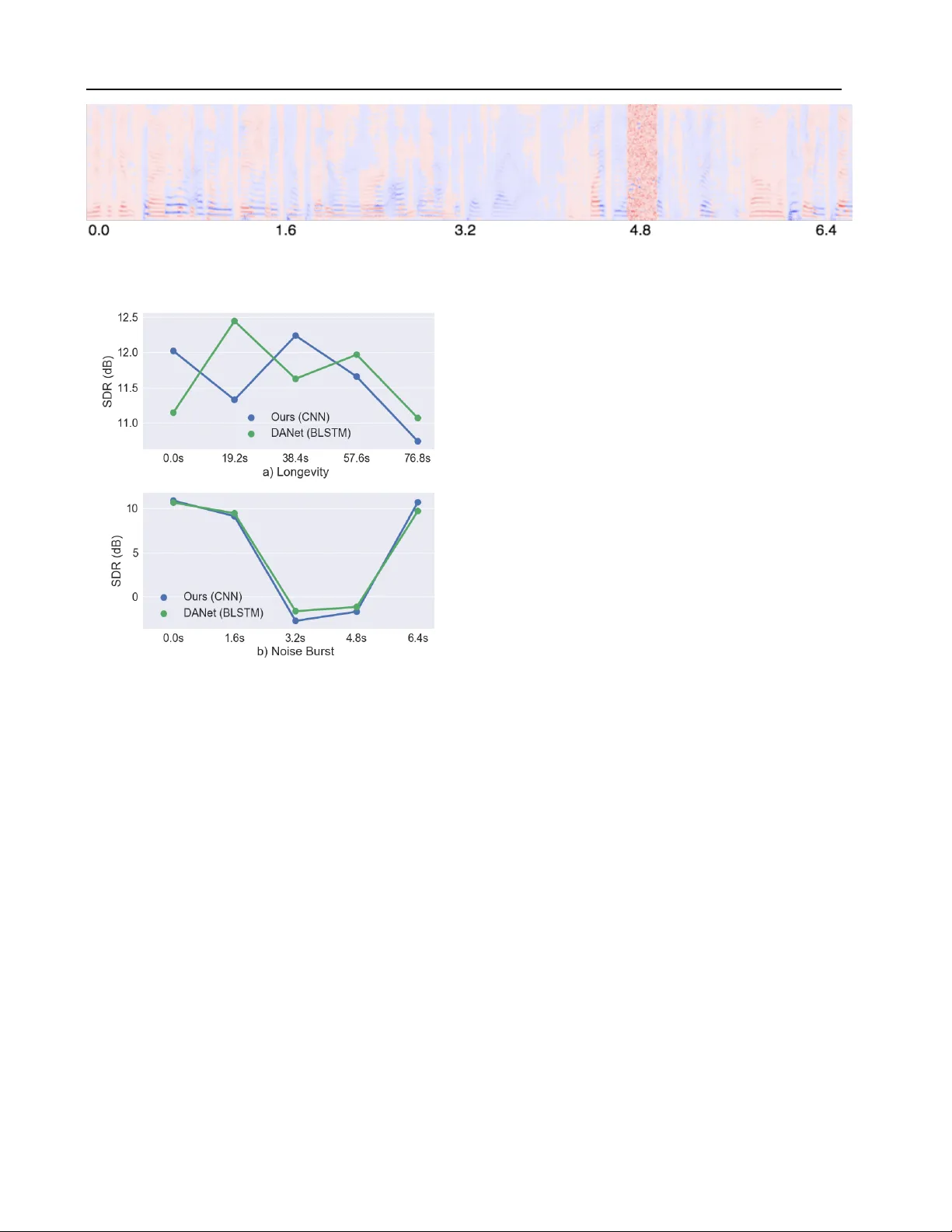
Generalization Challenges f or Neural Ar chitectures in A udio Source Separation Shariq Mobin * 1 2 Brian Cheung * 1 2 Bruno Olshausen 1 2 Abstract Recent work has sho wn that recurrent neural net- works can be trained to separate individual speak- ers in a sound mixture with high fidelity . Here we explore con volutional neural network mod- els as an alternativ e and sho w that they achie ve state-of-the-art results with an order of magni- tude fe wer parameters. W e also characterize and compare the robustness and ability of these differ- ent approaches to generalize under three different test conditions: longer time sequences, the addi- tion of intermittent noise, and dif ferent datasets not seen during training. For the last condition, we create a new dataset, RealT alkLibri , to test source separation in real-world en vironments. W e show that the acoustics of the en vironment ha ve significant impact on the structure of the wav e- form and the overall performance of neural net- work models, with the con volutional model sho w- ing superior ability to generalize to ne w en viron- ments. The code for our study is av ailable at https://github .com/ShariqM/source separation. 1. Introduction The sound wa veform that arriv es at our ears rarely comes from a single isolated source, but rather contains a complex mixture of multiple sound sources transformed in differ - ent ways by the acoustics of the en vironment. One of the central challenges of auditory scene analysis is to separate the components of this mixture so that individual sources may be recognized. Doing so generally requires some form of prior kno wledge about the statistical structure of sound sources, such as common onset, co-modulation and continu- ity among harmonic components ( Bregman , 1994 ; Darwin , 1997 ). Our goal is to develop a model that can learn to exploit these forms of structure in the signal in order to ro- bustly se gment the time-frequenc y representation of a sound wa veform into its constituent sources (see Figure 1 ). * Equal contribution 1 Redwood Center for Theoretical Neuro- science 2 Univ ersity of California Berkeley . Correspondence to: Shariq Mobin < shariqmobin@berkeley .edu > . Figure 1. Left and right column : T w o examples of source s epara- tion using the spectrogram of tw o ov erlapped v oices as input. F irst r ow : Spectrogram of the mixture. Second Row : The source esti- mates using the oracle (red and blue). Thir d Row : Source estimates using our method. The problem of source separation has traditionally been ap- proached within the frame work of computational auditory scene analysis (CASA) ( Hu & W ang , 2013 ). These methods typically rely upon features such as gammatone filters in order to find a representation of the data that will allo w for clustering methods to segment the individual speakers of the mixture. In some cases, these features are parameter- ized to allow for learning ( Bach & Jordan , 2006 ). Other approaches use generativ e models such as factorial Hidden Markov Models (HMMs) to accomplish speech separation or recognition ( Cooke et al. , 2010 ). Sparse non-negativ e matrix factorization (SNMF) ( Le Roux et al. , 2015 ) and Bayesian non-parametric models such as ( Nakano et al. , 2011 ) hav e also been used. Howe ver the computational complexity inherent in many of these approaches makes them difficult to implement in an online setting that is both robust and ef ficient. Recently , Hershey et al. ( 2016 ) introduced Deep Cluster- Generalization Challenges for Neural Architectures in A udio Source Separation ing (DPCL) which uses a Bi-directional Long short-term memory (BLSTM) ( Gra ves et al. , 2005 ) neural netw ork to learn useful embeddings of time-frequency bins of a mix- ture. They formulate an objectiv e function which encour- ages these embeddings to cluster according to their source so that K-means can be applied to partition the source sig- nals in the mixture. This model was further improved in the work of Isik et al. ( 2016 ) and Chen et al. ( 2017 ) which proposed simpler end-to-end models and achiev ed an im- pressiv e ∼ 10.5dB Signal-to-Distortion Ratio (SDR) in the source estimation signals. In this work we develop an alternative model for source separation based on a dilated con volutional neural netw ork architecture ( Y u & K oltun , 2015 ). W e show that it achiev es similar state-of-the-art performance as the BLSTM model with an order of magnitude fe wer parameters. In addition, our conv olutional approach can operate over a streaming signal enabling the possibility of source separation in real- time. Another goal of this study is to examine how well these different neural network models generali ze to inputs that are more realistic. W e test the models with inputs containing very long time sequences, intermittent noise, and mixtures collected under different recording conditions, including our RealT alkLibri dataset. Success in these more challeng- ing domains is critical for progress to continue in source separation, where the ev entual goal is to be able to separate sources regardless of speaker identities, recording devices, and acoustical en vironments. Figure 2 shows three exam- ples of ho w these factors can af fect the spectrogram of the recorded wa veform. While the Automatic Speech Recognition (ASR) community has begun to discuss and address this generalization chal- lenge ( V incent et al. , 2017 ; Hsu et al. , 2017 ), there has been less discussion in the context of audio source separation. In vision and machine learning, this issue is usually referred to as dataset bias ( T orralba & Efros , 2011 ; Tzeng et al. , 2017 ; Donahue et al. , 2014 ) where models perform well on their training dataset but f ail to generalize to new datasets. In re- cent years the main approach to tackling this issue has been through data augmentation. In the speech community , sim- ulators for dif ferent acoustical en vironments ( Barker et al. , 2015 ; Kinoshita et al. , 2013 ) hav e been le veraged to create more data. Here we show that the choice of model architecture alone can improv e generalization. Our choice to use a conv olu- tional architecture was inspired by the generalization po wer of Conv olutional Neural Networks (CNNs) ( LeCun et al. , 1998 ; Krizhevsky et al. , 2012 ; Sigtia et al. , 2016 ) relati ve to fully connected networks. W e compare the performance of our CNN model with the recurrent BLSTM models of previous w ork and show that while both suf fer when tested Figure 2. a : Original recording of a single female speaker from the LibriSpeech dataset; b,c,d : Recordings of the original wa veform made with three different orientations between computer speak er and recording device. on reaslistic mixtures under novel recording conditions, the CNN model degrades more gracefully and exhibits superior performance to the BLSTM in this regime. 2. Deep Attractor Framework Notation: For a tensor T ∈ R A × B × C : T · , · ,c ∈ R A × B is a matrix, and T a, · ,c ∈ R B is a vector , and T a,b,c ∈ R is a scalar . 2.1. Embedding the mixed wav eform Chen et al. ( 2017 ) propose a frame work for single-channel speech separation. x ∈ R τ is a raw input signal of length τ and X ∈ R F × T is its spectrogram computed using the Short-time Fourier transform (STFT). Each time-frequenc y bin in the spectrogram is embedded into a K-dimensional latent space V ∈ R F × T × K by a learnable transformation f ( · ; θ ) with parameters θ : ¯ V = f ( X ; θ ) (1) V f ,t, · = ¯ V f ,t, · || ¯ V f ,t, · || 2 (2) In our work, the embeddings are normalized to the unit sphere in the latent dimension k (eq. 2 ). 2.2. Generating embedding labels W e assume that each time-frequency bin can be assigned to one of the C possible speakers. The Ideal Binary Mask (IBM), ¯ Y ∈ { 0 , 1 } F × T × C , is a one-hot representation of Generalization Challenges for Neural Architectures in A udio Source Separation Figure 3. Overvie w of the source separation process. this classification for each time-frequency bin: ¯ Y f ,t,c =    1 , if c = arg max c 0 ( S f ,t,c 0 ) 0 , otherwise (3) where S ∈ R F × T × C is the supervised source target spec- trogram. W e estimate ¯ Y by a mask M ∈ (0 , 1) F × T × C computed from the spectrogram X . T o prevent time-frequency embeddings with negligible power from interfering, the raw classification tensor ¯ Y is first masked with a threshold tensor H ∈ R F × T . The threshold tensor removes time-frequenc y bins which are be- low a fraction 0 < α < 1 of the highest po wer bin present in X : H f ,t = ( 0 , if X f ,t < α max ( X ) 1 , otherwise (4) Y · , · ,c = ¯ Y · , · ,c  H (5) where  denotes element-wise product. 2.3. Clustering the embedding An attractor point, A c ∈ R K , can be thought of as a cluster center for a corresponding source c . Each attractor A c is the mean of all the embeddings which belong to speaker c : A c,k = P f ,t V f ,t,k Y f ,t,c P f ,t Y f ,t,c (6) During training the attractor points are calculated using the thresholded oracle mask, Y . In the absence of the oracle mask at test time, the attractor points are calculated using K- means. Only the embeddings which pass the corresponding time-frequency bin threshold are clustered. Finally the mask is computed by taking the inner product of all embeddings with all attractors and applying a softmax: M f ,t,c = sof tmax c  X k A c,k V f ,t,k  (7) From this mask, we can compute source estimate spectro- grams: ˆ S · , · ,c = M · , · ,c  X (8) which in turn can be con verted back to an audio wa veform via the inv erse STFT . W e do not attempt to compute the phase of the source estimates. Instead, we use the phase of the mixture to compute the inv erse STFT with the magnitude source estimate spectrogram ˆ S . The loss function L is the mean-squared-error (MSE) of the source estimate spectrogram and the supervised source target spectrogram, S ∈ R F × T × C : L = X c || S · , · ,c − ˆ S · , · ,c || 2 F (9) (10) where || · || F denotes the Frobenius norm. See Figure 3 for an ov erview of our source separation process. 2.4. Network Architecture A v ariety of neural network architectures are potential can- didates to parameterize the embedding function in Equation 2 . Chen et al. ( 2017 ) use a 4-layer Bi-Directional LSTM architecture ( Hochreiter & Schmidhuber , 1997 ; Schuster & Paliwal , 1997 ). This architecture utilizes weight sharing across time which allows it to process inputs of variable length. By contrast, con volutional neural networks are capable of sharing weights along both the time and frequency axis. Recently con volutional neural networks hav e been shown to perform state-of-the-art music transcription by having filters which con volv e ov er both the frequency and time di- mensions ( Sigtia et al. , 2016 ). One reason this may be advantageous is that the harmonic series exhibits a sta- tionarity property in the frequency dimension. Specifi- cally , for a signal with fundamental frequency f 0 the har- monics are equally spaced according to the follo wing set: { i ∗ f 0 : i = 2 , 3 , ..., n } . This structure can be seen in the equal spacing of successiv e harmonics in Figure 2 d. Another motiv ation we ha ve for using con volutional neural Generalization Challenges for Neural Architectures in A udio Source Separation networks is that they do not incorporate feedback which may allow them to be more stable under novel conditions not seen during training. In the absence of a recurrent memory , filter dilation ( Y u & K oltun , 2015 ) enables the receptiv e field to integrate information ov er long time sequences without the loss of resolution. Furthermore, incorporating a fixed amount of future knowledge in the network is straightfor- ward by ha ving a fixed-lag delay in the con v olution as we show in Figure 4 . This is similar to fixed-lag smoothing in Kalman filters ( Moore , 1973 ). 3. Our Model 3.1. Dilated Con volution Y u & K oltun ( 2015 ) proposed a dilation function D ( · , · , · ; · ) to replace the pooling operations in vision tasks. For no- tational simplicity , we describe dilation in one dimension. This method con volv es an input signal X ∈ R G with a filter K ∈ R H with a dilation factor d : F t = D ( K, X, t ; d ) = X dh + g = t K h X g The input recepti ve field of a unit F t in an upper layer of a dilated con volutional network grows exponentially as a function of the layer number as shown in Figure 4 . When applied to time sequences, this has the useful property of encoding long range time dependencies in a hierarchical manner without the loss of resolution which occurs when using pooling. Unlike recurrent networks which must store time dependencies of all scales in a single memory vector , di- lated con v olutions stores these dependencies in a distrib uted manner according to the unit and layer in the hierarchy . Lower layers encode local dependencies while higher layers encode longer range global dependencies. Such models hav e been successfully used for generating audio directly from the raw wa veform ( Oord et al. , 2016 ). 4. Datasets W e construct our mixture data sets according to the proce- dure introduced in ( Hershey et al. , 2016 ), which is generated by summing two randomly selected wav eforms from dif- ferent speakers at signal-to-noise ratios (SNR) uniformly distributed from -5dB to 5dB and do wnsampled to 8kHz to reduce computational cost. A training set is constructed using speakers from the W all Street Journal (WSJ0) training dataset ( Garofalo et al. , 2007 ) si tr s. W e construct three test sets: 1) In WSJ0, a test set is constructed identical to the test set introduced in ( Hershey et al. , 2016 ) using 18 unheard speakers from si dt 05 and si et 05. Figure 4. One-dimensional, fixed-lag dilated con v olutions used by our model with dilation factors of 1, 2 and 4. The bottom row represents the input and each successive row is another layer of con volution. This network has a fixed-lag of 4 timepoints before it can output a decision for the current input. 2) In LibriSpeech, a test set is constructed using 40 unheard speakers from test-clean. 3) In RealT alkLibri , we generate more realistic mixture using the procedure described below . 4.1. RealT alkLibri Dataset The main motiv ation for creating this dataset is to record mixtures of speech where the acoustics of the room deform a high quality recording into a more realistic one. While datasets of real mixtures exist, there exists no dataset where the ground truth source wav eforms are av ailable, only the transcription of the speakers w ords are gi ven as tar get out- puts ( Kinoshita et al. , 2013 ; Barker et al. , 2015 ). In order to understand how well our model generalizes to real world mixtures we created a small test dataset for which there is ground truth of the source wa veforms. The RealT alkLibri (R TL) test dataset is created starting from the test-clean directory of the open LibriSpeech dataset ( Panayoto v et al. , 2015 ) which contains 40 speakers. W e first do wnsampled all wa veforms to 8kHz as before. Each mixture in the dataset is created by sampling two random speakers from the test-clean partition of LibriSpeech, picking a random wav eform and start time for each, and playing the wav eforms through two Logitech computer speakers for 12 seconds. The wa veforms of the two speak ers are played in separate channels linked to a left and right computer speaker , separated from the microphone of the computer by dif ferent distances. The recordings are made with a sample rate of 8kHz using a 2013 MacBook Pro (Figure 5 ). In order to obtain ground truth of the individual speaker wa veforms each of the w av eforms is played twice, once in isolation and once simultaneously with the other speaker . The first recording represents the ground truth and the second one is for the mixture. T o v erify the quality of the ground truth recordings, we constructed an ideal binary Generalization Challenges for Neural Architectures in A udio Source Separation T able 1: Dilated Con volution Model Architecture Layer 1 2 3 4 5 6 7 8 9 10 11 12 13 Con volution 3x3 3x3 3x3 3x3 3x3 3x3 3x3 3x3 3x3 3x3 3x3 3x3 3x3 Dilation 1x1 2x2 4x4 8x8 16x16 32x32 1x1 2x2 4x4 8x8 16x16 32x32 1x1 Residual False T rue F alse T rue False True False True F alse T rue False T rue False Channels 128 128 128 128 128 128 128 128 128 128 128 128 K mask ¯ Y which performs about as well on the previous simulated datasets, see the Oracle performance in Figure 9 . The RealT alkLibri data set is made up of two recording sessions which each yielded 4.5 hours of data, giving us a total of 9 hours of test data. The data is av ailable at https://www .dropbox.com/s/4pscejhkqdr8xrk/rtl.tar .gz?dl=0 Figure 5. Recording setup diagram. 5. Experiments 5.1. Experimental Setup W e ev aluate the models on a single-channel simultaneous speech separation task. The mixture wa veforms are trans- formed into a time-frequency representation using the Short- time Fourier T ransform (STFT) and the log-magnitude fea- tures, X , are served as input to the model. The STFT is computed with 32ms window length, 8ms hop size, and the Hann window . W e use SciPy ( Jones et al. , 2014 ) to com- pute the STFT and T ensorFlo w to build our neural networks ( Abadi et al. , 2016 ). W e report our results using a distance measure between the source estimate and the true source in the wav eform space. Our distance measure is the signal-to-distortion ratio (SDR) which was introduced in ( V incent et al. , 2006 ) as a blind audio source separation (BSS) metric which is less sensitiv e to the gain of the source estimate. W e compute our results using version 3 of the Matlab bsseval toolbox ( F ´ evotte et al. , 2005 ). A python implementation of this code is also av ailable online ( Raffel et al. , 2014 ) 1 . 1 https://github.com/craffel/mir_eval/ Our network consists of 13 dilated con volutional layers ( Y u & Koltun , 2015 ) made up of two stacks, each stack having its dilation factor double each layer . Batch Normal- ization ( Ioffe & Szegedy , 2015 ) is applied to each layer and residual connections ( He et al. , 2016 ) are used at every other layer , see T able 1 for details. Our model has a fixed- lag response of 127 timepoints ( ∼ 1s, see Figure 4 ). The output of the network is of dimensionality ( T × F × K ), T being the number of output time points, F the number of frequency bins, and K being both the final number of channels and embedding dimensionality . During training T is set to 400 ( ∼ 3s), F to 129 (specified by the STFT), K to 20, and α (threshold factor) to 0.6. For ev aluation we also use the max() function rather than the softmax() for computing the mask in equation ( 7 ). The Adam Opti- mizer ( Kingma & Ba , 2014 ) is used with a piecewise learn- ing rate schedule, boundaries = [10 k , 50 k , 100 k ] , values = [1 . 0 , 0 . 5 , 0 . 1 , 0 . 01] , and initial learning rate 1e − 3 . W e reimplement the D ANet of ( Chen et al. , 2017 ) with a BLSTM architecture containing 4 layers and 500 hidden units in both the forward and backward LSTM, for a total of 1000 hidden units. W e replicated their training schedule using the RMSProp algorithm ( T ieleman & Hinton , 2012 ), a starting learning rate of 1e − 3 , and e xponential decay with parameters: decay steps = 2000 , decay rate = 0 . 95 . W e calculate an Oracle score using the Ideal Binary Mask (IBM), ¯ Y , using the ground truth source spectrograms (Eq. 3 ). 5.2. WSJ0 Evaluation W e begin by e valuating the models on the WSJ0 test dataset as in ( Chen et al. , 2017 ). Our state-of-the-art results are shown in T able 2 . Our model achiev es the best score using a factor of ten fewer parameters than DANet. The DPCL score is taken from ( Isik et al. , 2016 ) which has a very sim- ilar architecture to D ANet and therefore a similar number of parameters. Their model has one important diff erence howe ver , a second neural network is used to enhance the source estimate spectrogram to achieve their result. Our blob/master/mir_eval/separation.py Generalization Challenges for Neural Architectures in A udio Source Separation model is still able to exceed its performance without this extra enhancement network. In addition, our model has a fixed windo w into the future whereas the BLSTM models hav e access to the entire future. This indicates that a con- volution based architecture is better at solving this source separation task with less information in comparison to a recurrent based architecture. T able 2: Signal-to-Distortion Ratio (SDR) for two competi- tor models, our proposed con volutional model, and the Ora- cle. Our model achieves the best results using significantly fewer parameters. Our score is averaged o ver 3200 exam- ples. *: SDR score is from ( Isik et al. , 2016 ). This model is at an adv antage because it has a second enhancement neural network that improv ed the source estimate spectrogram after masking in addition to the normal BLSTM. Model WSJ0 Number of SDR (dB) Parameters D ANet (BLSTM) 10.48 17 114 580 DPCL* (BLSTM) 10.8 ? Ours (CNN) 10.97 1 650 836 Oracle 13.49 - 5.3. Embeddings At test time we do not have access to the labels ¯ Y so the attractors cannot be computed using equation 6 . As in pre- vious work, K-means is employed instead. In order for the attractors to from a good proxy for the K-means algo- rithm it is important the attractors form dense clusters of embeddings. W ithout applying any re gularization on the at- tractors we found that this was not the case. The main issue we observed w as that embeddings for both speakers in the mixture were largely ov erlapping with a few embeddings driv en extremely far apart in order to drive the attractors apart. This worked well for training but poorly at test time, the solutions found by K-means didn’t match the attractors found in training. In order to combat this degeneracy we l2 normalize the embeddings V which is nov el and very effecti ve (Eq. 2 ). In Figure 6 we visualize the embedding outputs of our model using PCA for a single mixture across T = 200 timepoints. Each embedding point corresponds to a single time-frequency bin in the mixed input spectrogram. The em- beddings are colored in this diagram according to the oracle labelling, red for speaker 1 and blue for speaker 2. Notice that the network has learned to cluster the embeddings ac- cording to the speaker they belong too, i.e. there is a high density of red embeddings on the left and similarly for blue embeddings on the right. This structure allows K-means to easily find cluster centers that match the attractors used at Figure 6. Embeddings for two speakers (red & blue) o ver 200 time points, projected onto a 3-dimensional subspace using PCA. The orange points correspond to time-frequency bins where the energy was belo w threshold (see eq. 5 ). There are T × F = 200 × 129 = 25800 embedding points in total. training time. 5.4. Generalization Experiments 5 . 4 . 1 . L E N G T H G E N E R A L I Z A T I O N In the first experiment we study how well these models work under time-sequences 25x longer than they are trained on, i.e. T = 10000 ( ∼ 80 s). Previous work ( Kaiser & Sutske ver , 2015 ) has indicated that because recurrent ar- chitectures incorporate feedback they can function unpre- dictably for sequence lengths beyond those seen during training. On the other hand, con volutional network architec- tures do not incorporate an y feedback. This is adv antageous for processing time sequences of indefinite length because errors cannot accumulate ov er time. Since a conv olutional network is a stationary process in the con volv ed dimension, we hypothesize this architecture will operate more robustly ov er sequence lengths much longer than those seen during training. Our results are shown in Figure 8 a. Surprisingly , the results indicate that the BLSTM is also able to generalize to sequences of significantly lar ger length, contrary to our expectations. W e discuss possible explanations of this result in the next section. Our CNN model is able to maintain its performance across the long sequence as expected. 5 . 4 . 2 . N O I S E G E N E R A L I Z ATI O N In the second experiment we are interested in ho w the mod- els respond to small bursts of input data far outside of the training distribution. W e believ e the BLSTM model might become unstable as a result of such inputs because its re- current structure makes it possible for the noise to affect its hidden state indefinitely . W e took sequences of length T = 1200 ( ∼ 9 s) and inserted white noise for 0.25s in the middle of the mixture to disrupt the models process. Our Generalization Challenges for Neural Architectures in A udio Source Separation Figure 7. Source separation spectrogram for the noise generalization experiment. Figure 8. Results of the length and noise generalization experi- ments. For both plots, we plot the SDR starting at the time spec- ified by the x-axis up until 400 time points ( ∼ 3 s) later . Both the BLSTM and CNN are (a) able to operate o ver v ery long time sequences and (b) recover from intermittent noise. See Figure 7 for the spectrogram in b). results are sho wn in Figure 8 b. Again, contrary to our be- lief the BLSTM is very resilient to this noise, the model quickly reco vers after the noise passes (last data point). One possible explanation is that the BLSTM is only inte grating information over short time scales and therefore “forgets” about previous input data after a short number of time steps. W e believ e this is because when we construct the input for our models we randomly sample a starting time for each wa veform. This may force the BLSTM to learn a stationary function since it must be able to separate the mixture with or without information from the past in its hidden state. 5 . 4 . 3 . D AT A G E N E R A L I Z A T I O N In the final experiment we are interested in how well the models generalize to data progressiv ely farther from their training distrib ution. W e trained all the models on the WSJ0 training set and then tested on the WSJ0 test set, the Lib- riSpeech test set, and RealT alkLibri test set. Our results are shown in Figure 9 . Our model generalizes quite well from the WSJ0 dataset to the LibriSpeech dataset, only losing 1 . 8 dB of performance. Unfortunately it degrades substan- tially , by 7 . 5 dB, when using the R TL dataset. Howe ver , our model still outperforms the DANet model on all datasets. Note that the Oracle performance also de grades by ∼ 1 dB on R TL. In Figure 10 we visualize the mistakes our netw ork makes under the RealT alkLibri dataset. The first example indicates that the model does not have a strong enough bias to the harmonic structure contained in speech, it classifies the fre- quencies of the fundamental to a dif ferent speaker than the harmonic frequencies of that fundamental. The second ex- ample indicates that the model also has issues with temporal continuity , the speaker identity of particular frequency bins varies sporadically across time. This indicates that there is still room to improv e generalization in these models by modifying model architecture and adding regularization. 6. Discussion Recurrent neural networks ha ve been sho wn to perform au- dio source separation with high fidelity . Here we explored using con volutional neural networks as an alternati ve model. Our state-of-the-art results on the WSJ0 dataset using a fac- tor of ten fewer parameters sho w that con volutional models are both more accurate and more ef ficient for audio source separation. Our model has the additional advantage of work- ing online with a fixed-lag response of ∼ 1 sec. In order to study the robustness of all models we studied their performance under three dif ferent conditions: longer time sequences, intermittent noise, and datasets not seen during training. Our results in the length and noise gen- eralization experiments indicate that the BLSTM learns to behav e much like a stationary process in the temporal di- mension. W e do not observe any substantial de gradation in performance after it has been perturbed with noise. It also performs consistently on sequences which are significantly longer than those seen during training. Generalization Challenges for Neural Architectures in A udio Source Separation Figure 9. Results of models tested on WSJ0 simulated mixtures, LibriSpeech simulated mixtures, and our RealT alkLibri (R TL) dataset. Our model performs the best on WSJ0, generalizes better to LibriSpeech, but fails alongside the BLSTM at generalizing to the real mixtures of R TL. All models are trained on WSJ0. *: Model has a second neural network to enhance the source estimate spectrogram and is therefore at an adv antage. The model wasn’t av ailable online for testing against LibriSpeech or R TL. On the other hand, we get this stationarity property for free with our con volutional model. This further motiv ates our network architecture in Figure 4 which, by design, inte grates only local information from the past and future. In the final experiment we sho wed that our con volutional neural network also generalized better to both the Lib- riSpeech dataset and the RealT alkLibri dataset we intro- duced here. Models which are robust to new datasets as well as the deformations caused by the acoustics of dif fer- ent environments are critical to progress in audio source separation. Our RealT alkLibri dataset complements other real-world speech datasets ( Barker et al. , 2015 ; Kinoshita et al. , 2013 ) by additionally providing approximate ground truth wa veforms for the mixture which is currently not a vail- able. Looking forward, we aim to improve the generalization ability on examples such as those shown in Figure 10 by in- troducing a training set for RealT alkLibri , dev eloping more robust model architectures, introducing regularizers for the structure of speech, and creating powerful data augmenta- tion tools. W e also believ e models which can operate under an unkno wn number of sources is of utmost importance to the field of audio source separation. Figure 10. Left and right column : T wo examples of source sep- aration on the RealT alkLibri dataset. Row 1 : Source estimates using the oracle. Row 2 : The source estimates using our method. The model has difficulty maintaining continuity of speaker identity across frequencies of a harmonic stack (left column) and across time (right column). References Abadi, Mart ´ ın, Barham, Paul, Chen, Jianmin, Chen, Zhifeng, Davis, Andy , Dean, Jeffrey , Devin, Matthieu, Ghema wat, Sanjay , Irving, Geoffre y , Isard, Michael, et al. T ensorflow: A system for large-scale machine learning. In OSDI , volume 16, pp. 265–283, 2016. Bach, Francis R and Jordan, Michael I. Learning spectral clustering, with application to speech separation. Journal of Machine Learning Resear ch , 7(Oct):1963–2001, 2006. Barker , Jon, Marxer , Ricard, V incent, Emmanuel, and W atanabe, Shinji. The third chimespeech separation and recognition challenge: Dataset, task and baselines. In Au- tomatic Speech Recognition and Under standing (ASR U), 2015 IEEE W orkshop on , pp. 504–511. IEEE, 2015. Bregman, Albert S. Auditory scene analysis: The per ceptual or ganization of sound . MIT press, 1994. Chen, Zhuo, Luo, Y i, and Mesgarani, Nima. Deep attractor network for single-microphone speaker separation. In Acoustics, Speech and Signal Pr ocessing (ICASSP), 2017 IEEE International Confer ence on , pp. 246–250. IEEE, 2017. Cooke, Martin, Hershey , John R, and Rennie, Steven J. Monaural speech separation and recognition challenge. Computer Speech & Languag e , 24(1):1–15, 2010. Darwin, Chris J. Auditory grouping. T r ends in cognitive sciences , 1(9):327–333, 1997. Donahue, Jef f, Jia, Y angqing, V inyals, Oriol, Hof fman, Judy , Zhang, Ning, Tzeng, Eric, and Darrell, Tre vor . Decaf: Generalization Challenges for Neural Architectures in A udio Source Separation A deep con volutional activation feature for generic vi- sual recognition. In International conference on machine learning , pp. 647–655, 2014. F ´ evotte, C ´ edric, Gribon val, R ´ emi, and V incent, Emmanuel. Bss ev al toolbox user guide–revision 2.0. 2005. Garofalo, John, Graf f, David, Paul, Doug, and Pallett, David. Csr-i (wsj0) complete. Linguistic Data Consortium, Philadelphia , 2007. Grav es, Alex, Fern ´ andez, Santiago, and Schmidhuber , J ¨ urgen. Bidirectional lstm networks for impro ved phoneme classification and recognition. Artificial Neu- ral Networks: F ormal Models and Their Applications– ICANN 2005 , pp. 753–753, 2005. He, Kaiming, Zhang, Xiangyu, Ren, Shaoqing, and Sun, Jian. Deep residual learning for image recognition. In Pr oceedings of the IEEE conference on computer vision and pattern r ecognition , pp. 770–778, 2016. Hershey , John R, Chen, Zhuo, Le Roux, Jonathan, and W atanabe, Shinji. Deep clustering: Discriminative em- beddings for segmentation and separation. In Acoustics, Speech and Signal Pr ocessing (ICASSP), 2016 IEEE In- ternational Confer ence on , pp. 31–35. IEEE, 2016. Hochreiter , Sepp and Schmidhuber, J ¨ urgen. Long short-term memory . Neural computation , 9(8):1735–1780, 1997. Hsu, W ei-Ning, Zhang, Y u, and Glass, James. Unsuper- vised domain adaptation for robust speech recognition via variational autoencoder -based data augmentation. arXiv pr eprint arXiv:1707.06265 , 2017. Hu, Ke and W ang, DeLiang. An unsupervised approach to cochannel speech separation. IEEE T ransactions on audio, speech, and languag e pr ocessing , 21(1):122–131, 2013. Ioffe, Ser gey and Szegedy , Christian. Batch normalization: Accelerating deep network training by reducing internal cov ariate shift. In International Confer ence on Machine Learning , pp. 448–456, 2015. Isik, Y usuf, Roux, Jonathan Le, Chen, Zhuo, W atanabe, Shinji, and Hershey , John R. Single-channel multi- speaker separation using deep clustering. arXiv pr eprint arXiv:1607.02173 , 2016. Jones, Eric, Oliphant, Tra vis, and Peterson, Pearu. { SciPy } : open source scientific tools for { Python } . 2014. Kaiser , Ł ukasz and Sutske ver , Ilya. Neural gpus learn algo- rithms. arXiv preprint , 2015. Kingma, Diederik P and Ba, Jimmy . Adam: A method for stochastic optimization. arXiv pr eprint arXiv:1412.6980 , 2014. Kinoshita, K eisuke, Delcroix, Marc, Y oshioka, T akuya, Nakatani, T omohiro, Sehr , Armin, Kellermann, W alter , and Maas, Roland. The re verb challenge: A common e val- uation framew ork for derev erberation and recognition of rev erberant speech. In Applications of Signal Pr ocessing to Audio and Acoustics (W ASP AA), 2013 IEEE W orkshop on , pp. 1–4. IEEE, 2013. Krizhevsk y , Alex, Sutske ver , Ilya, and Hinton, Geof frey E. Imagenet classification with deep con volutional neural networks. In Advances in neural information pr ocessing systems , pp. 1097–1105, 2012. Le Roux, Jonathan, W eninger, Felix J, and Hershey , John R. Sparse nmf–half-baked or well done? Mitsubishi Elec- tric Resear ch Labs (MERL), Cambridge , MA, USA, T ech. Rep., no. TR2015-023 , 2015. LeCun, Y ann, Bottou, L ´ eon, Bengio, Y oshua, and Haffner , Patrick. Gradient-based learning applied to document recognition. Pr oceedings of the IEEE , 86(11):2278–2324, 1998. Moore, John B. Discrete-time fixed-lag smoothing algo- rithms. Automatica , 9(2):163–173, 1973. Nakano, Masahiro, Le Roux, Jonathan, Kameoka, Hirokazu, Nakamura, T omohiko, Ono, Nobutaka, and Sagayama, Shigeki. Bayesian nonparametric spectrogram modeling based on infinite factorial infinite hidden mark ov model. In Applications of Signal Processing to A udio and Acous- tics (W ASP AA), 2011 IEEE W orkshop on , pp. 325–328. IEEE, 2011. Oord, Aaron van den, Dieleman, Sander, Zen, Heiga, Si- monyan, Karen, V inyals, Oriol, Grav es, Alex, Kalch- brenner , Nal, Senior , Andrew , and Kavukcuoglu, Ko- ray . W avenet: A generativ e model for raw audio. arXiv pr eprint arXiv:1609.03499 , 2016. Panayoto v , V assil, Chen, Guoguo, Po ve y , Daniel, and Khu- danpur , Sanjeev . Librispeech: an asr corpus based on public domain audio books. In Acoustics, Speech and Signal Processing (ICASSP), 2015 IEEE International Confer ence on , pp. 5206–5210. IEEE, 2015. Raffel, Colin, McFee, Brian, Humphrey , Eric J, Salamon, Justin, Nieto, Oriol, Liang, Dawen, Ellis, Daniel PW , and Raffel, C Colin. mir ev al: A transparent implementation of common mir metrics. In In Pr oceedings of the 15th International Society for Music Information Retrieval Confer ence, ISMIR . Citeseer, 2014. Generalization Challenges for Neural Architectures in A udio Source Separation Schuster , Mike and Paliwal, Kuldip K. Bidirectional re- current neural networks. IEEE T ransactions on Signal Pr ocessing , 45(11):2673–2681, 1997. Sigtia, Siddharth, Benetos, Emmanouil, and Dixon, Simon. An end-to-end neural network for polyphonic piano mu- sic transcription. IEEE/A CM T ransactions on Audio, Speech and Language Pr ocessing (T ASLP) , 24(5):927– 939, 2016. T ieleman, T ijmen and Hinton, Geoffre y . Lecture 6.5- rmsprop: Divide the gradient by a running av erage of its recent magnitude. COURSERA: Neural networks for machine learning , 4(2):26–31, 2012. T orralba, Antonio and Efros, Alexei A. Unbiased look at dataset bias. In Computer V ision and P attern Recogni- tion (CVPR), 2011 IEEE Confer ence on , pp. 1521–1528. IEEE, 2011. Tzeng, Eric, Hoffman, Judy , Saenko, Kate, and Darrell, T rev or . Adversarial discriminativ e domain adaptation. In Computer V ision and P attern Recognition (CVPR) , volume 1, pp. 4, 2017. V incent, Emmanuel, Gribon val, R ´ emi, and F ´ evotte, C ´ edric. Performance measurement in blind audio source separa- tion. IEEE transactions on audio, speech, and langua ge pr ocessing , 14(4):1462–1469, 2006. V incent, Emmanuel, W atanabe, Shinji, Nugraha, Aditya Arie, Barker , Jon, and Marxer , Ricard. An analysis of en vironment, microphone and data simulation mismatches in robust speech recognition. Computer Speech & Languag e , 46:535–557, 2017. Y u, Fisher and K oltun, Vladlen. Multi-scale context aggregation by dilated conv olutions. arXiv preprint arXiv:1511.07122 , 2015.