FastFCA-AS: Joint Diagonalization Based Acceleration of Full-Rank Spatial Covariance Analysis for Separating Any Number of Sources

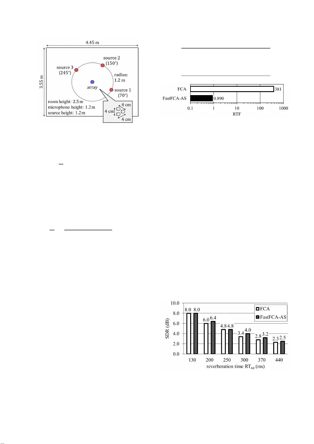
F ASTFCA-AS: JOINT DIA GONALIZA TION B ASED A CCELERA TION OF FULL-RANK SP A TIAL CO V ARIANCE AN AL YSIS FOR SEP ARA TING ANY NUMBER OF SOURCES Nobutaka Ito, T omohiro Nakatani NTT Communication Science L abo rato ri es, NTT Corporation, Kyoto, Japan { ito.nobutaka, nakatani.to mohiro } @lab .ntt.co.j p ABSTRA CT Here we propose F astFCA-A S , an accelerated algorithm for Full- rank spatial Covarian ce Analysis (FCA) , which is a robust audio source separation method prop osed by Duong et al. [“Under- determined reverb erant audio source separation using a full-rank spatial cov ariance model, ” IEEE Tr ans. ASLP , vol. 18 , no. 7, pp. 1830–1 840, Sept. 2010]. In the con vention al FCA, matrix in ver- sion and matrix multi plication are requ ired at each time-frequenc y point in each iteration of an iterative p arameter estimation algorithm. This causes a heavy computational load, thereby rendering th e F CA infeasible in many applications. T o ov ercome this drawback, we take a joint diag onalization app roach, where by matrix inv ersion and matrix multiplication are reduced to mere in version and multiplica- tion of diagonal entries. This makes the FastFCA-AS significantly faster than the FC A and e ven applicab le to observ ed data of long duration or a situation with restricted computational resources. Al- though we ha ve already proposed another acceleration of the FCA for two sources, the proposed FastFCA-AS is applicable to an arbi- trary number of sources. In an experiment with three sources and three microph ones, the FastFCA-AS was o ver 420 times f aster than the FCA with a sl i ghtly better s ource se paration p erformance. Index T erms — Micropho ne arrays, source separation, joint di- agonalization. 1. INTRODUCTION Duong et al. [1] hav e proposed a robust audio source separation method, which is called Full-ran k spatial Covaria nce Analysis (FCA) in this paper . The FCA performs source separation by us- ing the multichannel W iener filter optimal in the Minimum Mean Square Error (MMSE) sense. T o design the multichannel W iener filter properly , i t is crucial to ac curately estimate the covarian ce ma- trices of the source signals. In the FCA, these co va riance matrices are estimated fro m t he observed signals b y the maximum likeliho od method b ased on the Expectation -Maximization (EM) alg orithm. A major drawback of the FCA is expensi ve computation. Indeed, the abov e E M algorithm in volv es inv ersi on and multiplication of cov ari- ance matrices at each t ime-frequenc y point in each iteration. Since each of these matrix operation s requires computation of complex- ity O ( I 3 ) ( I : the matrix order) and the number of time-frequenc y points is normally huge, the FCA suf fers from a heavy computa- tional load. This may render t he FCA inapplicable to observed data of l ong duration or a situation with restricted comp utational re- sources, suc h as hearing aids, distributed microphone arrays, online speech enhancement, etc . In the two-source case, the above issue is addressed by a re- cently dev eloped accelerated algorithm for the FCA based on j oint diagonalization by the generalized eigen va lue problem [2, 3]. This method exploits the well-kno wn property that, for diago nal matri- ces, matrix in version and matrix multiplication are reduced to mere in version and multiplication of diagonal entries. Owing to this prop- erty , the joint diagonalization redu ces the comp utational comple xity of matrix inv ersion and matrix multiplication from O ( I 3 ) to O ( I ) . Consequently , t he compu tation time of the FC A is curtailed signif- icantly . Howe ver , this method has a significant drawback of being only applicable to t wo source s. Hence, we hereafter refer to this method as F astFCA -TS (Fast FC A for T wo Sources). T o accelerate the FC A ev en when the number of sources exceeds two, here we prop ose F astFCA- AS (Fast FCA for an Arbitrary num- ber of Sources). S i nce joint diagonalization based on t he generalized eigen value problem is inapplicable to such a case, we introduce an alternativ e wa y of joint diagonalization. Specifically , joint d iagonal- ization of the co v ariance matrices of the source signals is realized by maximum lik elihood estimation of a basis-transform matrix for joint diagonalization and the diagonalized cov ariance matrices. W e propose a hybrid algorithm combining the EM algorithm and the fixed point iteration for the maximum li kelihoo d parameter estima- tion. Conseq uently , the proposed FastFCA-AS leads to significantly accelerated source separation e ven when the n umber of sources ex- ceeds two. W e follow the following con ventions in this paper . Signals are represented in the Short-Time Fou rier T ransform (STFT) dom ain, where the time and the frequency indices are deno ted by n and f respecti vely . The numb er of frames is denoted by N , and the num- ber of frequenc y bins up to the Nyquist frequenc y by F . 0 denotes the column zero vector of an appropriate dimension, I the i dentity matrix of an appropriate order , diag ( α ) t he diagon al matrix whose diagonal entries are given by the vector α , ( · ) T transposition, ( · ) H Hermitian transposition, tr ( · ) the trace, and det( · ) the determinant. ‘ α , β ’ mea ns that α is defined by β . The rest of this pape r is organized as follo ws. Section 2 for- mulates the source separation problem we deal with in this paper . Section 3 revie ws the con ventional FCA. Section 4 describes the proposed FastFCA-AS. Section 5 describes experimental ev aluation, and finally S ection 6 concludes this paper . 2. PROBLEM FORMULA TION Suppose J source signa ls are observ ed by I microphones. Let y i ( n, f ) ∈ C d enote the observ ed signal at the i th microphone and y ( n, f ) ,  y 1 ( n, f ) y 2 ( n, f ) . . . y I ( n, f )  T the observed signals at all I microphones. W e model y ( n, f ) by the sum of J components x j ( n, f ) ( j = 1 , 2 , . . . , J ) co rresponding to the J source signals: y ( n, f ) = P J j =1 x j ( n, f ) . The components x j ( n, f ) ( j = 1 , 2 , . . . , J ) are called sour ce ima ges . The source separation prob lem we deal with in this paper is one of estimating x j ( n, f ) ( j = 1 , 2 , . . . , J ) from y ( n, f ) . 3. FCA: FULL-RANK SP A TIAL CO V ARIANCE ANAL YSIS 3.1. Full-Rank Spatial Cov ariance Model The FCA assumes that x j ( n, f ) ( j = 1 , 2 , . . . , J ; n = 1 , 2 , . . . , N ; f = 1 , 2 , . . . , F ) independently follow the zero-mean complex Gaussian distribution: p ( x j ( n, f )) = N ( x j ( n, f ); 0 , R j ( n, f )) . (1) Here, N ( α ; m , R ) denotes t he complex Gaussian distribution wi th mean m and co v ariance matrix R for a rand om vector α , and R j ( n, f ) denotes the co varianc e matrix of x j ( n, f ) . I mportantly , R j ( n, f ) is assumed to be parametrized as R j ( n, f ) = v j ( n, f ) | {z } po wer spe ctrum × S j ( f ) | {z } spatial characteristics , (2) where S j ( f ) m odels the spatial characteristics of t he j th sou rce sig- nal, and v j ( n, f ) the po wer spectrum of the j t h source signal. The matrix S j ( f ) i s called a spatial covariance matrix , and assumed to be Hermiti an, positi ve definite (and thus full-rank). T he parameter v j ( n, f ) is assumed to be positi ve. 3.2. Maximum Likelihood Estimation of Model Parame ters Once the model parameters S j ( f ) a nd v j ( n, f ) hav e been obtained, the s ource image x j ( n, f ) can b e estimated, e.g., by the M MSE es- timator (also known as the multi channel W iener fil t er): ˆ x j ( n, f ) = R j ( n, f ) J X k =1 R k ( n, f ) ! − 1 y ( n, f ) , (3) where R j ( n, f ) i s giv en by (2). Since the parameters S j ( f ) and v j ( n, f ) are not known a priori , they are estimated from the ob- served signals by the maximum likelihood method. This amounts to solving the follo wing o ptimization pro blem: max Θ L 1 (Θ) s.t . S j ( f ) ≻ 0 , v j ( n, f ) > 0 . (4) Here, Θ denotes the ensemble of the parameters S j ( f ) ( j = 1 , 2 , . . . , J ; f = 1 , 2 , . . . , F ) and v j ( n, f ) ( j = 1 , 2 , . . . , J ; n = 1 , 2 , . . . , N ; f = 1 , 2 , . . . , F ) , and L 1 (Θ) t he l og-likelihoo d func- tion: L 1 (Θ) , N X n =1 F X f =1 ln N y ( n, f ); 0 , J X j =1 v j ( n, f ) S j ( f ) ! . (5) ‘ A ≻ 0 ’ means that A i s a positive definite Hermitian matrix. 3.3. Expectation-Maximization Algorithm The FCA realizes the maximu m likelihood estimation by the EM algorithm [4], in w hich an Expectation step (E -step) and an Maxi- mization step (M-step) are iterated alternately . In the E-step, the current estimates of the parameters S j ( f ) and v j ( n, f ) are used to update the posterior probability p ( x j ( n, f ) | y ( n, f )) of x j ( n, f ) , which t urns out to be a complex Gaussian dis- tribution again: p ( x j ( n, f ) | y ( n, f )) = N ( x j ( n, f ); µ j ( n, f ) , Φ j ( n, f )) , (6) where µ j ( n, f ) denotes the mean and Φ j ( n, f ) the cov ariance matrix. Therefore, the E-step amounts to updating µ j ( n, f ) and Φ j ( n, f ) . This is done by the follo wing upd ate rules: µ j ( n, f ) ← R j ( n, f ) J X k =1 R k ( n, f ) ! − 1 y ( n, f ) , (7) Φ j ( n, f ) ← R j ( n, f ) − R j ( n, f ) J X k =1 R k ( n, f ) ! − 1 R j ( n, f ) , (8) where R j ( n, f ) is giv en by (2). Note that (7) coincides with the MMSE estimator in ( 3). In the M-step, the esti mates of the parameters S j ( f ) and v j ( n, f ) are updated using µ j ( n, f ) and Φ j ( n, f ) obtained in the E-step. The update rules are as fo llows: v j ( n, f ) ← 1 I tr  S j ( f ) − 1 ( µ j ( n, f ) µ j ( n, f ) H + Φ j ( n, f ))  , (9) S j ( f ) ← 1 N N X n =1 1 v j ( n, f ) ( µ j ( n, f ) µ j ( n, f ) H + Φ j ( n, f )) . (10) 3.4. Drawback A major drawback of the FCA is expensi ve computation. Indeed, each iteration of the abov e EM algorithm r equires matrix in version and matrix multiplication at each t ime-frequenc y po int as seen from (7) and (8). Indeed, each iteration requires ( J + N ) F matrix in- versions and 2 J N F matrix multiplications. For ex ample, for the experimen tal setting in Section 5: I = J = 3 ; N = 249 ; F = 512 , the number of matrix in versions is ( J + N ) F = 129024 per itera- tion, an d the number of matrix multiplications is 2 J N F = 764928 per iteration. 4. F ASTFCA-AS: A CCELERA TED FCA FOR AN ARBITRAR Y NUMBER OF SOURCES 4.1. Appro ach: Joint Diagonalization This section describes the p roposed Fas tFCA-AS , an accelerated version of the FCA applicab le t o an arbitrary number of sources. The FastFCA-AS exploits the well-kno wn fact that, for d iagonal matrices, matrix i nv ersion an d matrix multiplication are reduced to mere in version and multiplication of diagonal entries, which are both of comple xity O ( I ) instead of O ( I 3 ) . This implies that, i f R j ( n, f ) ( j = 1 , 2 , . . . , J ) were all diagonal, matrix in version and matrix multiplication in (7) and (8) would be reduced to mere in- version and multiplication of diagon al entries. Ho wev er, elements of x j ( n, f ) (that is, the j th sou rce signal observed at differen t mi- crophones ) are no rmally mutually correlated, which implies that its cov ariance matrix R j ( n, f ) has non-zero off-diagon al entries. This motiv ates u s to consider joint diagonalization of t he spatial cov ariance matrices S j ( f ) ( j = 1 , 2 , . . . , J ) . That is, we con sider transforming S j ( f ) ( j = 1 , 2 , . . . , J ) into some diagonal matri ces Λ j ( f ) ( j = 1 , 2 , . . . , J ) by a single non-singular matrix P ( f ) as follo ws:      P ( f ) H S 1 ( f ) P ( f ) = Λ 1 ( f ) , · · · · · · P ( f ) H S J ( f ) P ( f ) = Λ J ( f ) . (11) For J = 2 sources, the gene ralized eigen value problem yields P ( f ) and Λ j ( f ) that satisfy (11) [5]. In the recently dev eloped FastFCA-TS [2, 3], this approach is employe d to accelerate t he F CA without degrading the source separation p erformance. Howe ver , the FastFCA-TS is limited t o the two-source case. For more than two so urces, the ge neralized eigen value prob lem based approach is inapplicable. Instead, in the proposed FastFCA- AS, S j ( f ) is assumed to be parametrized as      S 1 ( f ) = ( P ( f ) − 1 ) H Λ 1 ( f ) P ( f ) − 1 , · · · · · · S J ( f ) = ( P ( f ) − 1 ) H Λ J ( f ) P ( f ) − 1 . (12) (12) is obtained by solving ( 11) for S j ( f ) . The parameters P ( f ) , Λ j ( f ) , and v j ( n, f ) are estimated from the observed sign als by the maximum likelihoo d method. This makes it possible to accelerate the FCA e ven for more than tw o sources. 4.2. Objective Function The maximum likelihood method amounts to solving the follo wing optimization problem: max Ψ L 2 (Ψ) s.t. P ( f ) ∈ GL ( I , C ) , Λ j ( f ) ≻ 0 : diagon al , v j ( n, f ) > 0 . (13) Here, Ψ denotes the ensemb le of the parameters P ( f ) ( f = 1 , 2 , . . . , F ) , Λ j ( f ) ( j = 1 , 2 , . . . , J ; f = 1 , 2 , . . . , F ) , and v j ( n, f ) ( j = 1 , 2 , . . . , J ; n = 1 , 2 , . . . , N ; f = 1 , 2 , . . . , F ) . L 2 (Ψ) denotes th e l og-likelihoo d func tion: L 2 (Ψ) , N X n =1 F X f =1 ln N y ( n, f ); 0 , J X j =1 v j ( n, f )( P ( f ) − 1 ) H Λ j ( f ) P ( f ) − 1 ! . (14) GL ( I , C ) deno tes the set of the non-singular comple x matri ces of order I . 4.3. Optimization Algorithm The FastFCA-AS realizes t he maximum l ikelihood estimation by a hybrid algorithm combining the EM algorithm and the fixed po int iteration. In this algorithm, the following two steps are alternated: 1. Update Λ j ( f ) ( j = 1 , 2 , . . . , J ; f = 1 , 2 , . . . , F ) and v j ( n, f ) ( j = 1 , 2 , . . . , J ; n = 1 , 2 , . . . , N ; f = 1 , 2 , . . . , F ) by applying one iteration of the E M algorithm. 2. Update P ( f ) ( f = 1 , 2 , . . . , F ) by the fix ed point iteration. 4.3.1. EM-Based Λ j ( f ) and v j ( n, f ) Upd ate The EM-based Λ j ( f ) and v j ( n, f ) update consists of the E -step and the M-step described in the following. In th e E -step, the posterior probability p ( x j ( n, f ) | y ( n, f )) of x j ( n, f ) ( j = 1 , 2 , . . . , J ; n = 1 , 2 , . . . , N ; f = 1 , 2 , . . . , F ) i s updated based on the current parameter estimates. As in t he con- vention al F CA, p ( x j ( n, f ) | y ( n, f ) ) turns out to be a complex Gaussian distribution g iv en b y (6) with the mean µ j ( n, f ) given by (7) and the co varian ce matrix Φ j ( n, f ) by (8). Unlike the FCA, ho wev er, R j ( n, f ) in ( 7) and (8) is giv en by R j ( n, f ) = v j ( n, f )( P ( f ) − 1 ) H Λ j ( f ) P ( f ) − 1 . (15) Substitution of (1 5) i nto (7) a nd (8) yields P ( f ) H µ j ( n, f ) | {z } ˜ µ j ( n, f ) = v j ( n, f ) Λ j ( f ) J X k =1 v k ( n, f ) Λ k ( f ) ! − 1 P ( f ) H y ( n, f ) | {z } ˜ y ( n, f ) , (16) P ( f ) H Φ j ( n, f ) P ( f ) | {z } ˜ Φ j ( n, f ) = v j ( n, f ) Λ j ( f ) − v j ( n, f ) Λ j ( f ) J X k =1 v k ( n, f ) Λ k ( f ) ! − 1 ( v j ( n, f ) Λ j ( f )) . (17) Therefore, ˜ µ j ( n, f ) and ˜ Φ j ( n, f ) , basis-transformed versions of µ j ( n, f ) and Φ j ( n, f ) , can be updated by (16) and (17), in which matrix in version and matrix multiplication are of comp lexity O ( I ) instead of O ( I 3 ) owing to the joint diagonalization. In the M-step, v j ( n, f ) ( j = 1 , 2 , . . . , J ; n = 1 , 2 , . . . , N ; f = 1 , 2 , . . . , F ) and Λ j ( f ) ( j = 1 , 2 , . . . , J ; f = 1 , 2 , . . . , F ) are up- dated based on maximization of the fo llowing Q-function: Q (Ψ) = − N X n =1 F X f =1 J X j =1 " ln det  v j ( n, f )( P ( f ) − 1 ) H Λ j ( f ) P ( f ) − 1  + t r  ( v j ( n, f ) Λ j ( f )) − 1  ˜ Φ j ( n, f ) + ˜ µ j ( n, f ) ˜ µ j ( n, f ) H   # . (18) Partial dif ferentiation wit h respect to v j ( n, f ) and Λ j ( f ) leads to the following update rules: v j ( n, f ) ← 1 I tr  Λ j ( f ) − 1 ( diag ( | ˜ µ j ( n, f ) | 2 ) + ˜ Φ j ( n, f ))  , (19) Λ j ( f ) ← 1 N N X n =1 1 v j ( n, f ) ( diag ( | ˜ µ j ( n, f ) | 2 ) + ˜ Φ j ( n, f )) , (20) where | · | 2 is computed in an en try-wise ma nner . 4.3.2. F ixed P oint Iter ation Based P ( f ) Update The bas is-transform matrix P ( f ) ( f = 1 , 2 , . . . , F ) is updated based o n the fixed point iteration applied to the lo g-likelihood func- tion (14). Partial differen tiation (the ma trix Wirtinger deriv ative [6]) of (14) wit h respect to the complex conjugate P ( f ) ∗ of P ( f ) is gi ven by ∂ L 2 (Ψ) ∂ P ( f ) ∗ = N ( P ( f ) − 1 ) H − N X n =1 y ( n, f ) y ( n, f ) H P ( f ) J X j =1 v j ( n, f ) Λ j ( f ) ! − 1 . (21) Fig. 1 . Experimental setti ng (bird’ s e ye view). Setting (21) to zero and v ectorizing bo th sides of the equation yields vec ( P ( f )) = " 1 N N X n =1 J X j =1 v j ( n, f ) Λ j ( f ) ! − 1 ⊗  y ( n, f ) y ( n, f ) H  # − 1 vec  ( P ( f ) − 1 ) H  (22) o wing to the formula vec ( AXB ) = ( B T ⊗ A ) v ec ( X ) . Here, vec denotes th e opera tor that stacks the column v ectors of the input ma- trix, and ⊗ the K r oneck er prod uct. Noting th e block diagonal struc- ture, we can re write (22) as follo ws: [ P ( f )] i ← " 1 N N X n =1 1 P J j =1 v j ( n, f )[ Λ j ( f )] ii y ( n, f ) y ( n, f ) H # − 1 ×  ( P ( f ) − 1 ) H  i . (23) Here, [ A ] i denotes the i th colum n of the matrix A , and [ A ] il the ( i, l ) -entry of the matrix A . The fixed point iteration consists in iterating (23). 4.4. Advantage The proposed Fa stFCA includes o nly ( I + 1) F K matrix in versions per iteration of t he hybrid algorithm and no matrix multiplications, where K denotes the number of iterations in the fixed point iteration. Note that, unlike the FCA, the number of matrix in versions does not depend on N , which is typically large. Here, matrix in versions and matrix multiplications for diagona l matrices were not counted, because their comp utational complexity is O ( I ) instead of O ( I 3 ) . For the e xperimental setti ng in Section 5 where K = 1 , the number of matrix in versions is o nly ( I + 1) F K = 204 8 per iteration of the hybrid algorithm. 4.5. Discussion Here we described the hybrid algorithm combining the EM algo- rithm and the fixed point it erati on. Ot her optimization techn iques could also be employed. For example, the fixed point iteration f or updating P ( f ) could be replaced by the gradient method, the natural gradient method, Newton’ s method, etc. W e could also employ the normal EM al gorithm, in which P ( f ) is also updated in th e M-step. T ab le 1 . Experimental co nditions. sampling frequency 16 kHz frame length 1024 (64 ms) frame shift 512 (32 ms) windo w square root o f Han n number of iterations 20 Fig. 2 . Real Time Factor (RTF). 5. EXPERIMENT AL EV ALU A TION W e cond ucted a source separation experimen t to comp are the pro- posed FastFCA-AS with the FCA [1] (see Section 3). These meth- ods were implemented in MA T LAB (R2013a) and run on an Intel i7-2600 3.4-GHz octal-core CPU. Obse rved signals were g enerated by con volving 8 s-long English speech signals with room impulse responses [7] measured in an experiment room. The locations of the sources and the microphon es are depicted in Fig. 1. The reve rbera- tion time R T 60 was 130, 200, 250, 3 00, 370, o r 440 ms, and for each rev erberation time, ten trials were condu cted with dif ferent comb i- nations of speech signals. The pa rameters were i nitialized b ased on mask-based cov ariance matrix estimation [8, 9] with the masks ob- tained by the method in [7]. The source images were estimated using the multichannel W iener filter in all algorithms. Some other condi- tions are fo und in T able 1. Figure 2 sho ws the Real Time Factor ( RTF) of the parameter es- timation average d over all ten tri als and all six re verberation times, and Figure 3 sho ws the Signal-to-Distortion Ratio (SDR) [10] aver- aged over all three sources and all ten t r ials. The proposed FastFCA- AS was over 420 times faster t han the FC A with its source separation performance slightly better than t he FCA. 6. CONCLUSIONS In th is p aper , we have proposed the FastFCA-AS, an accelerated al- gorithm for the FCA. Compared to t he con ventiona l FastFCA-TS, the FastFCA-AS has a major adv antage of being applicable to not only two sources b ut also more than two sources. Fig. 3 . Signal-to-Distortion Ratio ( S DR). 7. REFERENCES [1] N.Q.K. Duong, E. V incent, and R. Gribon val, “Under- determined rev erberant audio source separation using a full- rank spatial co va riance model, ” IEE E T rans. ASLP , vol. 18, no. 7, p p. 1 830–1840 , Sept. 2010. [2] N. Ito, S. Araki, and T . Nakatani, “FastFCA: A joint diagonal- ization based fast algorithm for audio source separation using a full-rank spatial cov ariance model, ” arXi v p r eprint , May 2018, arXiv : 180 5.06572. [3] N. Ito, S. Araki, and T . Nakatani, “FastFCA: Joint diagonal- ization based acceleration of audio source separation using a full-rank spatial cov ariance model, ” in Pr oc. EUSIPCO , Sept. 2018 (accepted). [4] A.P . Dempster, N.M. Laird, and D . B. R ubin, “Maximum like- lihood from i ncomplete data via the EM algorithm, ” Journa l of the R oyal Statistical Society: Series B (Methodolo gical) , vol. 39, no. 1, pp. 1–38, 1977. [5] G.H. Golub and C.F . V an Loan, Matrix Computations , The Johns Hopkins Un iv ersity P ress, Baltimore, 1983. [6] A. Hjørungnes and D. Gesbert, “Complex-v alued matrix dif- ferentiation: T echniques and key results, ” IEEE T rans. SP , vol. 55, no. 6, pp. 2740–27 46, June 2007. [7] H. Saw ada, S. Araki, and S. Makino , “Unde rdetermined con- voluti ve blind source separation via frequency bin-wise clus- tering and permutation alignment, ” IE EE Tr ans. ASLP , vol. 19, no. 3, pp. 516–527 , Mar . 20 11. [8] M. Souden, S. Ar aki, K. Kinoshita, T . Nakatani, and H. Sa wada, “ A multichannel MMSE-based fr amework for speech source separation and noise reduction, ” IEE E T rans. ASLP , vol. 21, no. 9, pp. 1913–1928 , Sept. 2013. [9] T . Y oshioka, N. Ito, M. Delcroix, A. Ogawa, K. Kinoshita, M. Fujimoto, C. Y u, W .J. Fabian, M. Espi, T . Higuchi, S . Araki, and T . Nakatani, “The NTT CHiME-3 system: Adv ances in speech enhancemen t and recognition for mobile multi- microphone devices, ” in Pr oc. ASR U , Dec. 2015, pp. 436–443. [10] E. V incent, R. G r i bon val, and C. F ´ evotte, “Performance mea- surement in blind audio source separation, ” IEEE T rans. ASLP , vol. 14, no . 4 , p p. 1 462–1469 , Jul. 2006.