Phase Transitions and a Model Order Selection Criterion for Spectral Graph Clustering

Phase T ransitions and a Model Or der Selec tion Criteri on for Spectral Graph Clustering Pin-Y u Chen and Alfred O. Hero I II, F ellow , IEEE Abstract —One of the longstandin g open pro blems in spectral graph clustering (SGC) is the so-called model order selection problem: automated selection of th e correct number of clusters. This is equivalent to th e problem of ﬁn ding the number of connected components or communities in an undi rected gra ph. W e propose automated model order selection (AMOS), a solution to the SGC model selection problem under a rand om intercon- nection model (RIM) usi ng a novel selection criterion th at is based on an asy mptotic phase transition analysis. AMOS can more generally be applied to discov ering hidden b l ock diagonal structure in symmetric non-negativ e matrices. Numerical experi- ments on simul ated graphs validate the p h ase transit i on a nalysis, and real-wor ld n etwork data is used to validate the performance of the p roposed model selection p rocedure . Index T erms —community detection, model selection, network analysis, phase t ransi t ion, spectral clustering I . I N T R O D U C T I O N Undirected grap hs are widely u sed for n e twork data anal- ysis, wher e nodes can repr esent entities or data samples, and the existence and strength of edges can represent relations or afﬁnity between nod es. For attributional data (e. g., multiv ariate data samp le s), su ch a grap h can be c onstructed by calcu la tin g and thresholding the similarity measure b e tween node s. For relational data (e.g ., friendships), the edges reveal the in ter- actions between n odes. The g o al o f grap h clustering is to group the no des into cluster s of high similarity . Applications of graph clustering , also known as commun ity detection [1], [2], include b ut a r e not limited to graph signal p rocessing [3]–[12], multiv ariate data clustering [1 3]–[15], im age segmentatio n [16], [17], stru ctural identiﬁability in phy sical systems [18], and network vulnerability assessment [19]. Spectral clustering [ 13]–[15] is a popular method for graph clustering, which we refer to as spectr a l grap h clustering (SGC). It works by transforming th e g raph ad jacency matrix into a graph Lap lacian matrix [ 2 0], compu ting its eigende- composition , and per forming K-m eans clusterin g [21] on th e eigenv ectors to par tition the nodes into clusters. Although heuristic methods have b e en proposed to automatically select the numb er of clusters [13], [1 4], [22], rigoro u s th eoretical justiﬁcations on the selection of the number of eigen vectors P .-Y . Chen is with IBM Thomas J. W atson Research Center , Y orkto wn Heights, NY 10598, USA. Em ail: pin-yu.chen@ibm.com. A. O. Hero is with the Department of Electric al Engine ering and Computer Scienc e, Univ ersity of Michigan, Ann Arbor , MI 48109, USA. E mail : hero@umich.edu . This work has been parti ally supported by the Army Researc h Ofﬁc e (AR O), grants W911NF-15-1 -0479 and W911NF-15-1-0241, and by the Consortium for V eriﬁca tion T echnology under Depart ment of Energy National Nuclea r Secu rity Admini stratio n, aw ard de-na0002534. This work w as con- ducted while P .-Y . Chen was at t he Univ ersity of Michigan, Ann Arbor, USA. Part of this work is presented at IEE E ICASSP 2017. for clusterin g a re still lack ing and little is known about the capabilities and limitations of spectral clustering on graphs. The contributions of this pap e r are twofold. First, we analyze the perfo r mance of spectral clustering on undirected unweighte d grap hs generated b y a r andom intercon n ection model (RIM), wh ere each clu ster can have arbitrary internal connectivity structure and the inter-cluster edges are assumed to be rando m. Under th e RIM, we establish a br eakdown condition on th e ab ility to id entify cor r ect clusters using SGC. Furthermore, wh en all of the cluster interconn e c tion probab ilities are iden tica l, a mod el we call the homogen eous RIM, this breakd own cond ition speciﬁes a critical p hase transition threshold p ∗ ∈ [0 , 1] on the in ter-cluster connection probab ility p . When th is interconnectio n pro bability is below the critical ph ase transition thresho ld, SGC can p e rfectly detect the clu sters. On th e oth er hand , when th e interconnection probab ility is above the critical p hase transition thresh old, SGC fails to identify the clusters. This b reakdown cond ition and phase tran sition an alysis a p ply to weig hted graphs as well, where th e cr itical ph ase tra nsition thr eshold depen ds not only on th e interco nnection proba bility but also on the weig hts of the interconne c tio n edg es. Second, we show that the phase tra nsition r e su lts for the homog eneous RIM can b e used to bound the phase tra nsitions of SGC for the inhomo geneou s RIM. T his leads to a method for automatically selecting th e number o f clusters in SGC, which we call autom ated m o del order selection (AMOS). AMOS works b y seque n tially increasing the mod el order while ru nning multi-stag e tests for testing for RIM structure . Speciﬁcally , fo r a given m odel or der an d an estimated cluster membersh ip map ob ta in ed from SGC, we ﬁrst test for local RIM structu re for a single clu ster pair u sing a b inomial test of homog eneity . Th is is re peated for all cluster pa ir s and, if they pass the RIM test, we proceed to the seco nd stage of testing, otherwise we incr ease the mo del orde r an d start ag ain. The second stage co n sists o f testing whether the RIM is g lo bally homog eneous or inho m ogeneo us. This is where the ph ase transition results are u sed - if an y of th e estimated inter-cluster connectio n pr o babilities exceed th e critical phase transition threshold the model order is increased. In this man ner, th e outputs fro m AMOS are the clusterin g results from SGC of minimal model order that are deemed reliable. Simulation results on bo th unweigh ted an d weighted gr aphs generated by different network mod els validate our phase transition an a lysis. Compa r ing to oth er grap h clustering meth - ods, experim ents on re a l-world network datasets show that the AMOS alg orithm indeed outp uts clusters that a r e more consistent with th e g round -truth meta informatio n. For exam- ple, whe n applied to network data with longitud e and latitude meta info rmation, such as the In te r net backbone map across North American and Euro p e, an d the Minnesota road map, the clusters identiﬁed by the AMOS algorithm are more consistent with known g eograp hic separa tio ns. The rest of this paper is organized as follows. Sec. II discusses previous work on ph ase transition and model order selection for graph clustering . Sec. III intro duces the RIM and the mathematical form u lation o f SGC. Sec. IV describes the breakd own con dition and p hase transition a n alysis of SGC , in- cluding unweighted and weighted g r aphs. Sec. V su m marizes the prop osed AMO S alg orithm for SGC. Sec. VI discusses numerical exp e r iments and compar isons on simulated g raphs and real-world datasets. Sec. VII concludes this paper . I I . R E L A T E D W O R K A. Pha se tr ansitions in graph clustering In recent y ears, research ers have established phase tran- sitions in the accuracy of graph clustering und er a d iv erse set of network models [2], [23]–[28]. A widely used network model is the stochastic block model ( SBM) [29], where the edge con nections within an d between clu sters are in d ependen t Bernoulli ran dom variables. Under the SBM, a ph ase transition on the clu ster interconnectivity p r obability sep arates clustering accuracy into two regimes: a regime wh ere c o rrect graph clustering is possible, and a regime wher e corr e c t gr aph clustering is impossible. The cr itica l values that separ a te these two regime s are called p h ase tran sition thresholds. A summary of ph ase transition analysis u nder the SBM can be found in [26]. In this pap er , we estab lish th e p hase transition an alysis of SGC under a mor e general network mo del, which we call the rando m interconnection model (RIM). The RIM does no t impose any distributional assump tions on the within-clu ster connectivity structure, but assumes the between- cluster edges are generated by a SBM. The form al deﬁnition of the RIM is introdu c ed in Sec. III-A. The RIM introdu ced in this paper is a direct gener alization of th e mod el introdu ced in [ 2], which is a special case of an unweig hted g r aph with two clu sters. B. Model order selec tio n criterion Most existing mo del selection algo rithms specify an upper bound K max on th e nu m ber K of clusters and th en select K based o n optimizing some objective function, e.g., the goodn ess o f ﬁt of th e k -cluster mod el f or k = 2 , . . . , K max . In [13], the o b jectiv e is to minimize the sum of cluster -wise Euclidean distances between each data point and the centroid obtained from K-mean s cluster in g. In [22], the objective is to maximize the gap b e twe en th e K -th largest and the ( K + 1 ) - th largest eig e n value. In [14], the auth ors propose to minimize an o bjectiv e fun ction th at is associated with th e cost of alignin g the eigenvectors with a canonical co o rdinate system. In [ 3 0]–[33], model selection is c a st as a multiscale commun ity de te c tion p roblem. In [34], the author s prop ose to iterativ ely divide a cluster based on the leading eig en vector of the modularity matrix until no signiﬁca n t improvement in the modular ity measur e can be achieved. The Louvain metho d in [35] uses a greedy algorithm for modu larity m a ximization. In [36], the authors use the integrated classiﬁcation likelihood (ICL) cr iterion [37] for graph clustering based a ran dom graph mix ture mo d el. In [38], the authors use the degree- corrected SBM [ 3 9] a n d Monte Carlo samp ling techniqu es for graph clustering . In [4 0], [41], the author s pro pose to use the eig en vectors of the nonback tracking m a tr ix for graph clustering, where the numbe r of clusters is determined by the number of re a l eig en values with mag nitude larger than the square r o ot o f th e largest eig en value. Different fro m these approa c h es, this paper not on ly establishes a new mo del order selection c riterion based o n the phase tran sition analysis, but also pr ovides multi-stage statistical tests for determining clustering reliability of SGC. I I I . R A N D O M I N T E R C O N N E C T I O N M O D E L ( R I M ) A N D S P E C T R A L C L U S T E R I N G A. Ran dom inter connection mo d el (RIM) Consider an undirected grap h where its connectivity struc- ture is repr esented by an n × n binary symmetric adjacency matrix A , where n is the number o f nodes in the graph. [ A ] uv = 1 if there exists an edge between the no de pair ( u, v ), and otherwise [ A ] uv = 0 . An unweig hted undirecte d graph is comp le te ly speciﬁed by its adjace ncy matrix A , while a weighted und irected graph is speciﬁed b y a nonnegati ve matrix W , wher e its nonzero entries deno te the we ig ht of an edge. In the n ext section , Theo rems 1 , 2 a n d 3 ap p ly to un weighted undirected graph s while Theorem 4 extends the se the o rems to weighted undirected graph s. Assume there a r e K clusters in the graph a n d deno te th e size of c lu ster k by n k . Th e size of the largest and smallest cluster is deno ted by n max and n min , respec ti vely . Let A k denote the n k × n k adjacency matrix repre sen ting the internal edge connectio ns in cluster k and let C ij ( i, j ∈ { 1 , 2 , . . . , K } ) be an n i × n j matrix representin g the adjacency matrix o f inter- cluster edge connectio n s between the cluster p air ( i, j ). The matrix A k is sym metric an d C ij = C T j i for all i 6 = j . Using these notations, th e a d jacency matrix of the en tir e grap h can be represented by a block structure, which is A =         A 1 C 12 C 13 · · · C 1 K C 21 A 2 C 23 · · · C 2 K . . . . . . . . . . . . . . . . . . . . . . . . . . . . . . C K 1 C K 2 · · · · · · A K         . (1) The proposed random interconnection mo del (RIM) a ssum es that: (1) the adjacency matrix A k is associated with a con- nected g raph of n k nodes but is othe rwise arbitrar y; (2) th e K ( K − 1) / 2 matrices { C ij } i>j are random and mutually indepen d ent, and each C ij has i.i.d. Bernoulli distributed en- tries with Bern oulli parame te r p ij ∈ [0 , 1] . W e call this m o del a homogeneous RIM when all rando m intercon nections have equal p robability , i.e., p ij = p for all i 6 = j . Oth e r wise, the model is called an in h omoge neous RIM. In the next section, Theorem s 1 and 3 a pply to general RIM while Theorems 2 and 4 are restricted to the homog eneous RIM. The stochastic block model (SBM) [29] is a special case of the RIM in the sen se that th e RIM d oes n ot impose any distributional con straints o n A k . In contrast, u nder the SBM A k is a Erdos-Renyi random graph with som e edg e conne c tion probab ility p k ∈ [0 , 1] . B. Spe c tral clustering Let 1 n ( 0 n ) b e the n -elemen t column vector of on es (zero s) and let D = diag ( d 1 , d 2 , . . . , d n ) be the diago nal degree matrix, where d = A1 n = [ d 1 , d 2 , . . . , d n ] T is the degree vector of the graph . The grap h Lap la c ian m atrix of the entire graph is de ﬁn ed as L = D − A , and similar ly the grap h Laplacian matrix of A k is d e n oted by L k . Let λ i ( L ) denote the i -th smallest eigenvalue of L . Then λ 1 ( L ) = 0 since L1 n = 0 n by deﬁnition, an d λ 2 ( L ) > 0 if the entire graph is connected . λ 2 ( L ) is also known as the algeb raic connectivity of the graph as it is a lower bound on the n ode and edg e connectivity of a connected g raph [42]. T o partition the nodes in the graph into K ( K ≥ 2 ) clusters, spectral clustering uses the K eig en vectors associated with the K smallest eigenvalues of L [15]. Each no d e can be viewed as a K -dim ensional vector in the subsp ace spann ed by these eigenv ectors. K-means clustering [2 1] is then implem ented on the K -dim ensional v ectors to group the nod e s into K clusters. V ector no rmalization of the obtain ed K -d imensional vectors or d egree normaliza tion of the adjacency matrix can be used to stabilize K-means clustering [13]–[15]. For analysis purpo ses, thr ougho ut this paper we will focus on th e case wh ere the ob served graph is connected . If the graph is not connecte d , th e connected components can be easily fo und and th e prop osed algorithm can be applied to each connected co mponen t separately . Since the smallest eigenv alue of L is always 0 an d the associated e igen vector is 1 n √ n , only the higher ord e r eigenvectors will affect the clustering results. By th e Cou rant-Fischer theorem [43], the K − 1 eig en vectors associated with the K − 1 smallest n onzero eigenv alues of L , represen ted by th e c o lumns o f the eige nvector matrix Y ∈ R n × ( K − 1) , are the solu tio n o f th e minim iza tion pro b lem S 2: K ( L ) = min X ∈ R n × ( K − 1) trace ( X T LX ) , subject to X T X = I K − 1 , X T 1 n = 0 K − 1 , (2) where the o ptimal value S 2: K ( L ) = trace ( Y T L Y ) = P K k =2 λ k ( L ) of ( 2) is the sum of the second to the K -th smallest e ig en values of L , and I K − 1 is th e ( K − 1) × ( K − 1) identity matr ix . The con straints in (2) impose or thonor m ality and centrality on the eigenv ectors. I V . B R E A K D OW N C O N D I T I O N A N D P H A S E T R A N S I T I O N A N A L Y S I S In this section we establish a mathematical condition ( The- orem 1) under which SGC fails to accurately identif y clusters under th e RIM. Furthe rmore, und er the h omogen eous RIM assumption of identical intercon nection p robability p ij = p governing the entries of the matrices { C ij } in (1), the condition leads to (Theorem 2) a critical phase tr a nsition threshold p ∗ where, if p p ∗ SGC fails. The phase tran sition analy sis developed in this section T ABLE I: Notation of limit expressions. expression limit value of ρ k n k n ρ max n max n ρ min n min n c n min n max c ∗ 1 n · min k ∈{ 1 , 2 ,.. . ,K } S 2: K ( L k ) c ∗ 2 1 n · min k ∈{ 1 , 2 ,.. .,K } λ 2 ( L k ) c ∗ K 1 n · min k ∈{ 1 , 2 ,.. .,K } λ K ( L k ) 1 ( 0 ) 1 n ( 0 n ) b p k L − e L k F n will b e used to establish an automated m o del orde r selection algorithm for SGC in Sec. V. The p roofs of the main the o rems (Theor e m s 1, 2 an d 3) are given in the appen dix, and the proof s of extended theorems an d corollaries are g i ven in the supplemen tary mate r ial. In the sequel, there are a numb e r of limit theo rems stated about th e b e havior of random m atrices an d vectors whose dimensions go to inﬁn ity as the sizes n k of the clusters goes to in ﬁnity while the ir relativ e sizes n k /n ℓ are held constant. Thr o ugho u t this pa p er , th e conver gence of a real matrix X ∈ R a × b is deﬁned with respect to the spectra l norm [44], deﬁned as k X k 2 = max z ∈ R b , z T z =1 k Xz k 2 , where k x k 2 denotes the Euc lid ean norm of the vector x . Let X = P r ( X ) i =1 σ i ( X ) u i ( X ) v T i ( X ) denote the sing ular value decom- position of X , where σ i ( X ) denotes the i -th largest singular value of X , u i ( X ) an d v i ( X ) are the associated le f t and right singular vectors, and r ( X ) den otes the rank o f X . F or any two matrices X and e X of the same dimension, we write X → e X if as n k → ∞ fo r a ll k , the spectral norm k X − e X k 2 , eq u iv alently σ 1 ( X − e X ) , conver ges to zer o. By W eyl’ s ine q uality [ 45], [46], X → e X implies X and e X asymptotically have the same singular values, i.e . , | σ i ( X ) − σ i ( e X ) | → 0 for all i ∈ { 1 , 2 , . . . , min( r ( X ) , r ( e X )) } , σ i ( X ) → 0 and σ i ( e X ) → 0 for all i > min( r ( X ) , r ( e X )) . Fu rthermor e, the Davis-Kahan theorem [46], [4 7] establishe s that under some mild con dition on the gap of singular values of X and e X , X → e X implies X and e X a symptotically h av e the same singular v ectors (iden tica l up to sign), i.e., | u T i ( X ) u i ( e X ) | → 1 and | v T i ( X ) v i ( e X ) | → 1 for all i ∈ { 1 , 2 , . . . , min( r ( X ) , r ( e X )) } . If X is a ran dom matrix and e X is a given matrix, th en X a.s. − → e X is shor th and for k X − e X k 2 → 0 almo st surely . In particular, if the dimension of X gr ows with n k , then for simplicity we often write X a.s. − → M , where M is a matrix o f inﬁnite dimension. For example, let I n denote the n × n identity ma tr ix. I f k X − I n k 2 a.s. − → 0 as n → ∞ , then for simp licity we write X a.s. − → I , wh ere I is the identity m atrix of inﬁnite d imension. While this inﬁnite dimension al n otation is non-rigoro us, its use in place of the mo r e cumber some notation k X − I n k 2 a.s. − → 0 greatly simpliﬁes the presentatio n. For vector s, we say x ∈ R n conv erges to e x ∈ R n if k x − e x k 2 → 0 as n → ∞ . Similarly , for a vector x , if k x − m n k 2 → 0 as n → ∞ , where m n is a v e c to r of in creasing dimension , we use the n otation x → m , where m is the inﬁnite dimension al limit of m n . T able I sum marizes the limit expressions p resented in this paper . Based o n the RIM (1), Theorem 1 establishes a gener al breakd own co ndition under which SGC fails to correctly identify the clusters. Theorem 1 (Breakdown condition ) . Let Y = [ Y T 1 , Y T 2 , . . . , Y T K ] T be the clu ster partitioned eigen v ector matrix associated with the graph Lap lacian matrix L obtained by solving (2), where Y k ∈ R n k × ( K − 1) with its r o ws indexing the nodes in cluster k . Let e A b e th e ( K − 1 ) × ( K − 1) matrix with ( i, j ) -th element [ e A ] ij =  ( n i + n K ) p iK + P K − 1 z =1 ,z 6 = i n z p iz , if i = j, n i · ( p iK − p ij ) if i 6 = j. The following holds almost sur ely as n k → ∞ and n min n max → c > 0 . If lim inf n →∞ 1 n min i ∈{ 1 ,...,K − 1 } , j ∈ { 2 , ...,K } | λ i ( e A ) − λ j ( L ) | > 0 , then Y T k 1 n k → 0 K − 1 , ∀ k ∈ { 1 , 2 , . . . , K } , and hence spectral graph clustering can not be successful. Since the eigenv alues of e A depend only on the RIM parameters p ij and n k whereas the eigenv alues of L d epend not only on these parameters but also on the interna l adjacen cy matrices A k , Theo rem 1 speciﬁes how the g r aph conn ectivity structure affects th e success of SGC. For the special case of homo geneou s RIM, where p ij = p , for all i 6 = j , Theor em 2 establishes the existence of a phase transition in the accuracy of SGC as the intercon nection probab ility p increases. A similar phase tran sition likely exists for the inhomog eneous RIM (i.e. , p ij ’ s ar e not id entical), but an inhomo geneou s extension of Theorem 2 is an op en problem . Non e th eless, Theo rem 3 sho ws that the h omogen eous RIM ph ase tran sition threshold p ∗ in Th eorem 2 can be used to bound clustering accuracy when the RIM is inhomog eneous. Theorem 2 (Phase tran sition ) . Let Y = [ Y T 1 , Y T 2 , . . . , Y T K ] T be the cluster partitioned eigen vector ma trix associated with the graph La placian matrix L ob tained b y solving (2), where Y k ∈ R n k × ( K − 1) with its r ows indexing th e nodes in cluster k . Let c ∗ = lim n →∞ 1 n · min k ∈{ 1 , 2 ,.. .,K } S 2: K ( L k ) a n d assume c ∗ 2 = lim n →∞ 1 n min k ∈{ 1 , 2 ,.. .,K } λ 2 ( L k ) > 0 . Und er the homogeneous RI M in (1) with con stant interconnection pr obab ility p ij = p , ther e e xists a critical value p ∗ such that the following holds almost sur ely as n k → ∞ and n min n max → c > 0 : (a)    If p ≤ p ∗ , S 2: K ( L ) n → ( K − 1) p ; If p > p ∗ , c ∗ + ( K − 1) (1 − ρ max ) p ≤ S 2: K ( L ) n ≤ c ∗ + ( K − 1) (1 − ρ min ) p. In particular , if p > p ∗ and c = 1 , S 2: K ( L ) n → c ∗ + ( K − 1) 2 K p . Furthermore , r eordering th e indices k in decreasing cluster size so that n 1 ≥ n 2 ≥ . . . ≥ n K , we have (b)                If p p ∗ , Y T k 1 n k → 0 K − 1 , ∀ k ∈ { 1 , 2 , . . . , K } ; If p = p ∗ , ∀ k ∈ { 1 , 2 , . . . , K } , √ n k Y k → 11 T K − 1 V k or Y T k 1 n k → 0 K − 1 , wher e V k = diag ( v k 1 , v k 2 , . . . , v k K − 1 ) ∈ R ( K − 1) × ( K − 1) is a diagonal matrix. F inally , p ∗ satisﬁes: (c) p LB ≤ p ∗ ≤ p UB , wher e p LB = c ∗ ( K − 1) ρ max and p UB = c ∗ ( K − 1) ρ min . In particular , p LB = p UB when c = 1 . Theorem 2 (a) establishes a ph ase transition of the partial eigenv alue sum S 2: K ( L ) n at some critical value p ∗ , called the critical ph ase transition threshold. When p ≤ p ∗ the quantity S 2: K ( L ) n conv e rges to ( K − 1 ) p . When p > p ∗ the slop e in p of S 2: K ( L ) n changes and the in te r cept c ∗ depend s o n the cluster having th e smallest partial eigen value su m . When all clusters have the same size (i.e., n max = n min = n K ) so th at c = 1 , S 2: K ( L ) n undergoes a slop e change from K − 1 to ( K − 1) 2 K . Theorem 2 (b) establishes that p > p ∗ renders the entries of the matrix Y k incohere n t, making it impossible for SGC to separate the clusters. On the oth er hand, p < p ∗ makes Y k coheren t, and h ence th e row vectors in the eigenv ecto r matrix Y p ossess cluster-wise sep arability . This is stated as follows . Corollary 1 (Separability of the ro w v e c tors in the eig en vecto r matrix Y w h en p 0 : (a) The columns of √ n k Y k ar e co nstant vectors. (b) Ea ch column of √ n Y has at least two nonzer o cluster -wise constant components, a nd these con stants ha ve a lternating signs such tha t their weighted sum eq u als 0 due to th e pr o perty P K k =1 v k j = 0 , ∀ j ∈ { 1 , 2 , . . . , K − 1 } . (c) No two column s of √ n Y have the same sign on the clu ster - wise nonzer o compon ents. These prop erties imply tha t for p < p ∗ the rows in Y k correspo n ding to dif fere n t n odes are id entical (Coro llary 1 (a)), while the r ow vectors in Y k and Y ℓ , k 6 = ℓ , corresp onding to different clusters are distinct (Coro llary 1 (b) and (c)). Therefo re, th e within -cluster distance betwee n any pair of row vectors in each Y k is zer o, wh e reas the between-cluster distance between any two row vectors of different clusters is nonzer o . T his mean s that a s n k → ∞ and n min n max → c > 0 the grou nd-tru th clusters be c o me the optimal solution to K- means clustering , a n d hence K-m eans clustering on th ese row vectors can g roup the nodes into correct clusters. Note that when p > p ∗ , from Theorem 2 (b) th e row vectors of Y k correspo n ding to the same cluster sum to a zero vector . T h is means tha t the entries o f each column in Y k have alternating signs and the c e ntroid of the r ow vectors of each clu ster is the origin. Ther efore, K-means clustering o n the rows of Y yields incorrect clusters. Furthermo re, as a demon stra tio n of the breakd own condition in Theorem 1, o bserve that when p ij = p , Theorem 1 implies that e A n is a diag o nal matrix p I K − 1 . From (2 0) in the append ix we k now that λ j ( L ) n → p for j = 2 , 3 , . . . , K almo st surely when p < p ∗ . The r efore, und er the hom ogeneou s RIM, SGC can only be successful when p is below p ∗ . Theorem 2 (c) p rovides u pper and lower bo unds o n the critical threshold value p ∗ for the phase tran sition to occur when p ij = p . These bound s are determined by the cluster having the smallest partial eigenv alue sum S 2: K ( L k ) , the number of clusters K , and th e size of th e largest an d smallest cluster ( n max and n min ). When a ll clu ster sizes are ide ntical (i.e., c = 1 ), these bo unds become tight. Based on Theorem 2 (c), the fo llowing c orollary speciﬁes the properties of p ∗ and the conn e ction to alg ebraic connectivity of each cluster . Corollary 2 (Pr o perties of p ∗ and its connection to algebraic connectivity) . Let c n = min k ∈{ 1 , 2 ,...,K } S 2: K ( L k ) n , c 2 ,n = min k ∈{ 1 , 2 ,...,K } λ 2 ( L k ) n and c K,n = min k ∈{ 1 , 2 ,...,K } λ K ( L k ) n , and let c ∗ , c ∗ 2 and c ∗ K denote their limit value, r espectively . Under the same assump - tions as in Theo r em 2, the fo llowing statements ho ld almo st sur ely as n k → ∞ and n min n max → c > 0 : (a) If c n = Ω  n max n  , then p ∗ > 0 . (b) If c n = o  n min n  , then p ∗ = 0 . (c) c ∗ 2 ρ max ≤ p ∗ ≤ c ∗ K ρ min . The fo llowing co r ollary speciﬁes the bo unds on the critical value p ∗ for some special types o f clusters. These results provide th eoretical justiﬁcation of the intu ition that strongly connected clusters, e .g., c omplete graphs, have hig h critical threshold value, and weak ly connected clusters, e.g., star graphs, have low critical threshold v alu e . Corollary 3 (bounds on the critical value p ∗ for special type of cluster) . Under the same assumptions as in Theor em 2, the following statements hold almost sur ely as n k → ∞ and n min n max → c > 0 : (a) If each cluster is a complete gr aph, then c ≤ p ∗ ≤ 1 . (b) If each cluster is a star gr aph, then p ∗ = 0 . Furthermo re, in the special case of a SBM, where each adjacency matrix A k correspo n ds to a Er dos-Renyi rando m graph with edge conn e ction pro b ability p k , under the same assumptions as in Theo rem 2 w e can sh ow that almost surely , c · min k ∈{ 1 , 2 ,.. .,K } p k ≤ p ∗ ≤ 1 c · m in k ∈{ 1 , 2 ,.. .,K } p k . (3) The proo f of (3) is given in the supplemen tary material. Similar resu lts for the SBM can also be ded uced from the latent space model [48]. The next coro llary summar izes the results from Theorem 2 for the case of K = 2 to elucidate the p hase tran sition pheno m enon. Note that it follows fro m Cor ollary 4 (b) th at below the p h ase transition ( p < p ∗ ) the rows in Y corre- sponding to d ifferent clusters are co nstant vector s with entries of opposite signs, and thus K-m eans clusterin g is cap able o f yielding corr ect clusters. On the oth er hand, above the ph ase transition ( p > p ∗ ) th e entries corresp onding to each cluster have alternating signs and th e centroid of each clu ster is the origin, and thus K-mean s clustering fails. Corollary 4 (Special case of Theorem 2 when K = 2 ) . When K = 2 , let Y = [ y T 1 y T 2 ] T , let c ∗ = lim n →∞ λ 2 ( L 1 )+ λ 2 ( L 2 ) −| λ 2 ( L 1 ) − λ 2 ( L 2 ) | 2 n and assume c ∗ 2 = lim n →∞ 1 n min { λ 2 ( L 1 ) , λ 2 ( L 2 ) } > 0 . Then th er e exists a critical value p ∗ such that the following hold s almost sur ely as n 1 , n 2 → ∞ and n min n max → c > 0 . (a) ( If p ≤ p ∗ , λ 2 ( L ) n → p ; If p > p ∗ , c ∗ + c 1+ c p ≤ λ 2 ( L ) n ≤ c ∗ + 1 1+ c p. (b) ( If p p ∗ , y T 1 1 n 1 → 0 and y T 2 1 n 2 → 0 . (c) p LB ≤ p ∗ ≤ p UB , wher e p LB = 2 c ∗ 1+ | ρ 1 − ρ 2 | and p UB = 2 c ∗ 1 −| ρ 1 − ρ 2 | . The ab ove p hase tran sition an a ly sis can also be applied to the inhomogeneo us RIM for which the p ij ’ s are not constant. Let p min = min i 6 = j p ij and p max = max i 6 = j p ij . The c o rollary below sho ws that und er the inhomo geneou s RIM whe n p max is b e low p ∗ , which is th e critical thresho ld value spec iﬁed by Th eorem 2 for the homogen eous RIM, the smallest K − 1 nonzer o eigenv alu es of the gr aph L aplacian matrix L n lie within the internal [ p min , p max ] with prob ability one. Corollary 5 (Bounds on the smallest K − 1 no nzero eigen- values of L u nder the inhomogen eous RIM) . Under the RIM with interconnection pr o babilities { p ij } , let p min = min i 6 = j p ij , p max = max i 6 = j p ij , and let p ∗ be the critical thr eshold value o f the homogeneo us RIM speciﬁed by Theor e m 2. If p max 0 : p min ≤ λ j ( L ) n ≤ p max , ∀ j = 2 , 3 , . . . , K. In particu lar , Corollar y 5 implies that the n ormalized al- gebraic con nectivity o f the inh omogen eous RIM λ 2 ( L ) n is between p min and p max almost surely as n k → ∞ an d n min n max → c > 0 . For g r aphs following the inhomoge n eous RIM, Theo rem 3 below establishes th at a c c urate clu stering is p ossible if it can b e determined tha t p max < p ∗ . As deﬁned in Theorem 2, let Y ∈ R n × ( K − 1) be the eigenvector matrix of L under the inho m ogeneo us RIM, and let e Y ∈ R n × ( K − 1) be the eigenv e c tor matrix of th e graph Lap lacian e L of an other random graph, indep endent of L , generated by a homo geneou s RIM with cluster intercon nectivity p a rameter p . W e can specify the distance between the subspaces spa n ned by the columns of Y a nd e Y by inspecting their principal angles [15]. Since Y an d e Y both have orth onorma l colu mns, th e vector v of K − 1 pr incipal angles between their co lumn spaces is v = [cos − 1 σ 1 ( Y T e Y ) , . . . , cos − 1 σ K − 1 ( Y T e Y )] T , where σ k ( M ) is the k -th largest singular value of a real rectangular matrix M . Let Θ ( Y , e Y ) = diag ( v ) , and let sin Θ ( Y , e Y ) b e d eﬁned entrywise. When p < p ∗ , the following theo rem p rovides an upper b o und on th e Froben ius norm of sin Θ ( Y , e Y ) , which is denoted by k sin Θ ( Y , e Y ) k F . Theorem 3 (Distance between column spaces spa n ned by Y and e Y ) . Un der th e RIM with interconnection pr obab ilities { p ij } , let p ∗ be the critical thr eshold value for the ho mo - geneous RIM speciﬁed by Theor em 2, a nd deﬁne δ p,n = min { p, | λ K +1 ( L ) n − p |} . F or a ﬁxed p , let b p denote the limit of k L − e L k F n . If p 0 as n k → ∞ , the follo wing statemen t hold s almo st sur ely as n k → ∞ and n min n max → c > 0 : k sin Θ ( Y , e Y ) k F ≤ b p δ p . (4) Furthermore , let p max = max i 6 = j p ij . If p max < p ∗ , k sin Θ ( Y , e Y ) k F ≤ min p ≤ p max b p δ p . As estab lished in Corollary 1, under the homo geneou s RIM when p 0 . Un der the inhom o geneou s RIM, Theorem 3 establishes that cluster separab ility can still b e expected pr ovided that k sin Θ ( Y , e Y ) k F is small an d p < p ∗ . As a result, we can bound the clustering accur acy u nder the inhomog eneous RIM by insp ecting the u pper bo und (4) on k sin Θ ( Y , e Y ) k F . No te that if p max < p ∗ , we can ob tain a tigh ter upp er boun d on (4). Next we e x tend Th eorem 2 to und irected weighted random graphs obeying the homog eneous RIM. T he edges within each cluster are assumed to hav e non negativ e weigh ts and the weights of in ter-cluster ed ges are assumed to be independently drawn fro m a com mon n onnegative bound ed distribution. Let W denote the n × n symmetric nonnegative weight ma tr ix of the entire graph . Then the cor respond in g graph Laplacian matrix is d eﬁned a s L = S − W , where S = diag ( W1 n ) is the diagonal matrix of n odal streng ths of the weighted graph. Similarly , the symmetric graph Lapla c ian matr ix L k of each cluster can be d e ﬁned. The follo win g theo rem establishes a phase transition phenomeno n for such weighted graphs. Speciﬁcally , the cr itical value depends no t o nly on the in ter- cluster edge connectio n probability but also on the mean of inter-cluster edge weig hts. Theorem 4 (Phase transition in weighted g raphs) . Und e r the same assumptions as in Theor em 2 , further assume the weight matrix W is symmetric, nonnegative and bound ed, an d the weigh ts o f the upp er triangular part o f W are in d ependen tly drawn fr om a commo n no nnegative bound ed distribution with mean W . Let t = p · W and c ∗ = lim n →∞ 1 n · min k ∈{ 1 , 2 ,.. . ,K } S 2: K ( L k ) . Then ther e exists a critical value t ∗ such th at the following holds almo st sur ely as n k → ∞ and n min n max → c > 0 : (a)    If t ≤ t ∗ , S 2: K ( L ) n → ( K − 1) t ; If t > t ∗ , c ∗ + ( K − 1) (1 − ρ max ) t ≤ S 2: K ( L ) n ≤ c ∗ + ( K − 1) (1 − ρ min ) t. (b)                If t < t ∗ , √ n k Y k → 11 T K − 1 V k =  v k 1 1 , v k 2 1 , . . . , v k K − 1 1  , ∀ k ∈ { 1 , 2 , . . . , K } ; If t > t ∗ , Y T k 1 n k → 0 K − 1 ∀ k ∈ { 1 , 2 , . . . , K } ; If t → t ∗ , ∀ k ∈ { 1 , 2 , . . . , K } , √ n k Y k → 11 T K − 1 V k or Y T k 1 n k = 0 K − 1 , wher e V k = diag ( v k 1 , v k 2 , . . . , v k K − 1 ) ∈ R ( K − 1) × ( K − 1) is a diagonal matrix. (c) t LB ≤ t ∗ ≤ t UB , wher e t LB = c ∗ ( K − 1) ρ max and t UB = c ∗ ( K − 1) ρ min . Theorem 1 and Theo rem 3 can be extended to weighted graphs under the inhomo g eneous RIM. Moreover , The orem 4 reduces to Theorem 2 when W = 1 . V . A U T O M AT E D M O D E L O R D E R S E L E C T I O N ( A M O S ) A L G O R I T H M F O R S P E C T R A L G R A P H C L U S T E R I N G Based on the phase transition analysis in Sec . IV, we pro- pose an auto m ated m o del o rder selection (AMOS) algorithm for selecting the numbe r of cluster s in spectral gr aph clusterin g (SGC). This algorithm prod u ces p-values of h ypothe sis tests                                 ! " # $ % & ' ( ) * + , - . / 0 1 2 3 4 5 6 7 8 9 : ; < = > ? @ A B C D E F G H I J K L M N O P Q R S T U V W X Y Z [ \ ] ^ _ ` a b c d e f g h i j k l m n o p q r s t u v w x y z { | } ~                                   ¡ ¢ £ ¤ ¥ ¦ § ¨ © ª « ¬  ® ¯ ° ± ² ³ ´ µ ¶ · ¸ ¹ º » ¼ ½ ¾ ¿ À Á Â Ã Ä Å Æ Ç È É Ê Ë Ì Í Î Ï Ð Ñ Ò Ó Ô Fig. 1: Flow dia g ram o f the pr oposed auto mated m odel order selection (AMOS) scheme in spectral graph cluster (SGC). for testing the RIM and phase tran sition. In particular, u nder the h omoge n eous RIM , we can estimate the critical phase transition threshold fo r each putative cluster f ound and use this estimate to construct a test of reliability of the cluster . The statistical tests in the AMOS algorithm are imp lemented in two phases. Th e ﬁrst phase is to test the RIM assumption based on th e interconne c ti v ity pattern o f each clu ster (Sec. V -B), and the second phase is to test the hom o geneity an d variation of th e interconn ectivity param eter p ij for e very cluster pair i and j in add ition to m aking comparison s to the critical phase transition thr eshold (Sec. V -C). The ﬂow diagram of the propo sed algo rithm is displayed in Fig. 1, and the algor ith m is summarized in Algorithm 2. The AMOS package is publicly av ailable for do wnload 1 . Next we explain th e f unctionality of each block in the diagram . A. Inp ut n etwork data and spectral clustering The input network data is a matrix that can b e a sym- metric adjacency matrix A , a degree - normalized symmetric adjacency matrix D − 1 2 AD − 1 2 , a sym metric weight matrix W , or a norm alized symmetr ic weigh t matrix S − 1 2 WS − 1 2 , where D = diag ( A1 n ) and S = diag ( W1 n ) are assumed in vertible . Spectral clustering is then implemen ted on the inp ut data to p roduc e K clu sters { b G k } K k =1 , wh ere b G k is the k - th identiﬁed cluster with number o f nodes b n k and number of edge s b m k . In itially K is set to 2 . Th e AMOS algorithm works by iter a tively incr easing K an d p erformin g spectral clustering on the data until the output clu sters meet a level of signiﬁcance cr iterion speciﬁed by the RIM test and phase transition estimator . B. RIM test via p-va lu e fo r local homogeneity testin g Giv en clusters { b G k } K k =1 obtained f r om spectr al clu stering with model order K , let b C ij be the b n i × b n j interconn ection matrix of edges con n ecting clu sters i and j . Our go al is to compute a p-value to test the h ypothesis th at th e matrix A in (1) satisﬁes the RIM. More speciﬁcally , we are testing the null hypoth esis that b C ij is a r ea lization of a rando m m a trix with i.i.d. Bernoulli entries (RIM) and the alternative hypo thesis that b C ij is n o t a r ea lization o f a random matrix with i.i.d. Bernoulli en tries entries (no t RIM), for all i 6 = j , i > j . Since the RIM ho mogene ity model fo r th e in terconne c tio n matrices { C ij } will only be valid when the clusters have been correc tly identiﬁed, this RIM test can be used to test th e quality o f a graph clustering algorithm. T o compute a p-value fo r the RIM we u se the V -test [49] f o r homog eneity testing of the r ow sum s or colum n sum s of b C ij . Speciﬁcally , given s indep endent b in omial r andom variables, 1 https:/ /github .com/tgensol/AMOS Algorithm 1 p-value computation of V -test for the RIM test Input: An n i × n j interconn ection m atrix b C ij Output: p-value ( i, j ) x = b C ij 1 n j (# of nonzero entries of each row in b C ij ) y = n j 1 n i − x (# of zero entries of each row in b C ij ) X = x T x − x T 1 n i and Y = y T y − y T 1 n i . N = n i n j ( n j − 1) and V =  √ X + √ Y  2 . Compute test statistic Z = V − N √ 2 N Compute p-value ( i , j )= 2 · min { Φ( Z ) , 1 − Φ( Z ) } Algorithm 2 Automated mode l ord er selection (AMOS) al- gorithm for spectral graph clustering (SGC) Input: a conne c ted un d irected weigh te d gra p h, p-value signiﬁcance le vel η , hom ogeneo us and inhomoge n eous RIM conﬁdenc e inte r val parameter s α , α ′ Output: number of clusters K and identity of { b G k } K k =1 Initialization: K = 2 . Flag = 1 . while Flag = 1 do Obtain K clusters { b G k } K k =1 via spectral clustering ( ∗ ) for i = 1 to K do for j = i + 1 to K do Calculate p-value( i, j ) fro m Algorithm 1. if p-value( i, j ) ≤ η then Reject RIM Go back to ( ∗ ) with K = K + 1 . end if end for end for Estimate b p , c W , { b p ij } , and b t LB speciﬁed in Sec. V -C. if b p lies within the conﬁdence interval in (5) then # Homogeneous RIM phase transition test # if b p · c W < b t LB then Flag = 0 . else Go ba c k to ( ∗ ) with K = K + 1 . end if else if b p does not lie within (5) then # Inho mogeneous RIM phase transition test # if Q K i =1 Q K j = i +1 F ij  b t LB c W , b p ij  ≥ 1 − α ′ then Flag = 0 . else Go back to ( ∗ ) with K = K + 1 . end if end if end while Output K clusters { b G k } K k =1 . the V -test tests that they are all identically distributed. For concreten ess, here we ap p ly the V -test to the row sums. Given a cand id ate set of clusters, the V -test is app lied indepen d ently to each of the  K 2  interconn ection matrices { b C ij } . For any interconnection matrix b C ij the test statistic Z of the V -test conv erges to a stand ard no rmal distribution as n i , n j → ∞ , an d the p-value for the hypoth esis that the row sums of b C ij are i.i.d. is p-value ( i, j ) = 2 · min { Φ( Z ) , 1 − Φ( Z ) } , where Φ( · ) is the cumu lati ve distribution fun ction (cdf ) of th e standard norm al d istribution. The pr oposed V - test procedu r e is summarized in Algorithm 1. The RIM te st on b C ij rejects the nu ll hypo thesis if p-value ( i, j ) ≤ η , wher e η is the desired single co m parison signiﬁcance level. Since the C ij ’ s are inde p endent, the p-value thre shold paramete r η can b e easily translated into a multiple comparisons signiﬁcance le vel for dete c tin g homog e n eity of all C ij ’ s. It can a lso be translated into a th reshold fo r testing the homogen eity of at least o ne of the se matr ices usin g family-wise error rate Bonfer roni correction s or false discovery rate a n alysis [50], [51]. C. A cluster quality measure for RIM Once the id e ntiﬁed clu sters { b G k } K k =1 pass the RIM test, one can e m pirically determin e the reliability of the clustering using the phase tr ansition analy sis introduced in the p r evious section. In a nutshell, if the estimate of p max = max i>j p ij falls below the critical phase transition threshold p ∗ then, by Theorem 3, the results of the clustering algorithm can be declare d reliab le if the clustering quality measure k sin Θ( Y , e Y ) k F is small. This is the basis fo r the propo sed AMOS p r ocedur e un d er the assumption of inho mogeneo us RIM. For homogen eous RIM models an alternative proc edure is prop osed. The AMOS algorithm (Fig. 1) runs a ser ia l proc e ss of h omogen eous and inhomo geneou s RIM phase tran sition tests. Each of these is considered separately in what follows. • Homogeneous RIM p h ase transition test : The following plug-in estimators are used to ev aluate the RIM parameters and the critical phase transition thre sh old u nder th e homog eneous RIM. L e t b m ij = 1 T n i b C ij 1 n j be the n umber o f inter-cluster edges between clu sters i and j (i.e., the nu m ber of nonzero entries in b C ij ). Then und er the in homog eneous RIM b p ij = b m ij b n i b n j is the m aximum likelihoo d estimator (MLE) of p ij . Under the h omogen eous RIM, p ij = p , and the MLE of p is b p = P K i =1 P K j = i + 1 b m ij P K i =1 P K j = i + 1 b n i b n j = 2( m − P K k =1 b m k ) n 2 − P K k =1 b n 2 k , where m is the numb e r of ed ges in the gr aph. W e use the estimates b p and { b p ij } to carry out a test for the h omogen eous RIM and utilize the estimated critical phase transition threshold developed in this paper to evaluate the clu stering quality when it p a sses the test. Intu itively , if { b p ij } are close to b p and b p is below th e estimated phase transition th reshold, then the ou tput clusters are regard ed h omogen eous an d reliab le. On the other hand, if there is a large v ar iatio n in { b p ij } , the homo g eneity test fails. A gen eralized log-likelihood ratio test (GLR T) is u sed to test the validity of th e h o mogen eous RIM. T he details are giv en in the su p plementar y mater ial. By the Wilk’ s theor em [52], an asymp totic 100(1 − α )% conﬁdence interv a l fo r p in an assumed homoge neous RIM is ( p : ξ ( K 2 ) − 1 , 1 − α 2 ≤ 2 K X i =1 K X j = i +1 I { b p ij ∈ (0 , 1) } [ b m ij ln b p ij +( b n i b n j − b m ij ) ln(1 − b p ij )] − 2 m − K X k =1 b m k ! ln p − " n 2 − K X k =1 b n 2 k − 2 m − K X k =1 b m k !# ln(1 − p ) ≤ ξ ( K 2 ) − 1 , α 2 ) , (5) where ξ q,α is the upper α -th quantile of the central chi-sq u are distribution with degree of free d om q . The clusters pass the homogeneo us RIM test if b p is within the conﬁden ce inter val (5), an d by Theo r em 2 th e clusters ar e deemed reliable if b p < b p LB , an estimate of the lower bou nd on the critical phase transition th reshold value, which is denoted by b p LB = min k ∈{ 1 , 2 ,...,K } S 2: K ( b L k ) ( K − 1) b n max . • Inho mogeneous RIM phase transition test : As estab lished in Theo rem 3, if max i>j p ij < p ∗ , we can o btain a tight bound on the cluster ing quality m easure k sin Θ( Y , e Y ) k F , and b y the per f ect separability in e Y from Theorem 2, we can conclude that the clusters identiﬁed by SGC are reliable. W e use the maximum of MLEs of p ij ’ s, denoted by b p max = max i>j b p ij , as a test statistic for testing the null hypoth esis H 0 : max i>j p ij j p ij ≥ p ∗ . The test accepts H 0 if b p max < p ∗ , and rejects H 0 otherwise. Using the Anscomb e transform ation on the b p ij ’ s fo r variance stabilizatio n [5 3], let A ij ( x ) = sin − 1 s x + c ′ b n i b n j 1+ 2 c ′ b n i b n j , wher e c ′ = 3 8 . By the cen- tral limit theo rem, p 4 b n i b n j + 2 · ( A ij ( b p ij ) − A ij ( p ij )) d − → N (0 , 1) f o r all p ij ∈ (0 , 1) as b n i , b n j → ∞ , where d − → denotes conver g ence in distribution an d N (0 , 1 ) denotes the stan dard nor m al distribution [53]. Th erefore, und e r the null hyp othesis that max i>j p ij < p ∗ , from [54, Th eo- rem 2.1] an asymptotic 1 00(1 − α ′ )% co nﬁdence in terval for b p max is [0 , ψ ] , where ψ ( α ′ , { b p ij } ) is a functio n of the precision param eter α ′ ∈ [0 , 1] and { b p ij } , which satisﬁes Q K i =1 Q K j = i +1 Φ  p 4 b n i b n j + 2 · ( A ij ( ψ ) − A ij ( b p ij ))  = 1 − α ′ , and Φ( · ) is the cdf of the standard no r mal distribution. Therefo re, if ψ < p ∗ , then b p max < p ∗ with probab ility at least 1 − α ′ . Note that verif ying ψ < p ∗ is eq uiv alent to checking the cond itio n K Y i =1 K Y j = i +1 F ij ( p ∗ , b p ij ) ≥ 1 − α ′ , (6) where F ij ( p ∗ , b p ij ) = Φ  p 4 b n i b n j + 2 · ( A ij ( p ∗ ) − A ij ( b p ij ))  · I { b p ij ∈ (0 , 1) } + I { b p ij

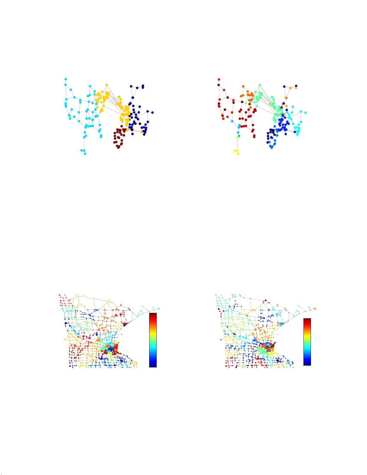
0 , where I is the identity matrix of inﬁnite d imension and d iag ( 1 n i ) = I n i → I a s n i → ∞ . T he con vergence resu lt in (15) can b e p roved u sing the fact that each entry of the vector C ij 1 n j is the sum of i.i.d. Bern oulli rand om variables an d k D ij n j − p ij I n i k 2 = max z ∈{ 1 , 2 ,...,n i } | [ D ij n j − p ij I n i ] z z | . Speciﬁcally , by Bernstein’ s concentr a tion ine quality [64], | [ D ij n j − p ij I n i ] z z | h as an ex- ponen tially decaying tail and hen ce by th e u nion bound , k D ij n j − p ij I n i k 2 a.s. − → 0 as n i , n j → ∞ . Using ( 15) and left multiplying (14) by 1 T n k n giv es 1 n   K X j =1 ,j 6 = k n j p kj 1 T n k Y k − K X j =1 ,j 6 = k n k p kj 1 T n j Y j − 1 T n k Y k U   a.s. − → 0 T K − 1 , ∀ k. (16) Using th e relation 1 T n K Y K = − P K − 1 j =1 1 T n j Y j , (16) can be represented as an asymptotic form of Sylvester’ s equatio n 1 n  e AZ − ZΛ  a.s. − → O , (17) where Z = [ Y T 1 1 n 1 , Y T 2 1 n 2 , . . . , Y T K − 1 1 n K − 1 ] T ∈ R ( K − 1) × ( K − 1) , e A is the ma trix speciﬁed in Theor e m 1, and we use the relation U = Λ = diag ( λ 2 ( L ) , λ 3 ( L ) , . . . , λ K ( L )) from (11). Let ⊗ denote the Kronecker pr oduct and let vec ( Z ) den ote the vectorization operation o f Z by stacking the columns of Z into a vector . (17) can be rep r esented as 1 n ( I K − 1 ⊗ e A − Λ ⊗ I K − 1 ) vec ( Z ) a.s. − → 0 , (18) where the matrix I K − 1 ⊗ e A − Λ ⊗ I K − 1 is the Kronecker sum, denoted by e A ⊕ − Λ . Observe that vec ( Z ) a.s. − → 0 is always a trivial solution to ( 18), an d if e A ⊕ − Λ is non- singular (i.e., its determinan t is nonzero), vec ( Z ) a.s. − → 0 is th e unique solution to (18). Sinc e vec ( Z ) a.s. − → 0 and P K k =1 1 T n k Y k = 0 T K − 1 imply 1 T n k Y k a.s. − → 0 T K − 1 for all k = 1 , 2 , . . . , K , the centroid 1 T n k Y k n k of each cluster in the eig e nspace is asymp to tically cen tered at the o rigin such that the clu sters are n ot pe r fectly separable, and hence accurate clustering is impo ssible. Therefore , a sufﬁcient condition fo r SGC u nder the RIM to fail is that th e matrix I K − 1 ⊗ e A − Λ ⊗ I K − 1 be non-singu lar . Moreover, using the proper ty of the Kro necker sum that the eigenv a lu es of e A ⊕ − Λ satisfy { λ ℓ ( e A ⊕ − Λ ) } ( K − 1) 2 ℓ =1 = { λ i ( e A ) − λ j ( Λ ) } K − 1 i,j =1 , the sufﬁcient con d ition on the failure of SGC under th e RIM is lim inf n →∞ 1 n min i,j | λ i ( e A ) − λ j ( L ) | > 0 for all i = 1 , 2 , . . . , K − 1 and j = 2 , 3 , . . . , K . B. Pr oo f of Theor em 2 Follo win g the deriv ation s in Appen d ix-A, since 1 T n k Y k = − P K j =1 ,j 6 = k 1 T n j Y j , und er the homogen eous RIM (i.e., p ij = p ), equation (16) can be simpliﬁed to  p I K − 1 − U n  Y T k 1 n k a.s. − → 0 K − 1 , ∀ k. (19) Below we fur ther di vid e the optimality c ondition in (19) into two cases b ased on wh ether Y T k 1 n k a.s. − → 0 n k for all k or not: Case 1:  p I K − 1 − U n  Y T k 1 n k a.s. − → 0 K − 1 , ∀ k and ∃ k s.t. lim n →∞ k Y T k 1 n k k 2 > 0; (20) Case 2: Y T k 1 n k a.s. − → 0 K − 1 , ∀ k. (21) Note that Case 1 immediately im plies U n a.s. − → p I K − 1 , which is proved a s follows. In Case 1, take a k such that  p I K − 1 − U n  Y T k 1 n k a.s. − → 0 K − 1 and lim n →∞ k Y T k 1 n k k 2 > 0 . Left multiplying  p I K − 1 − U n  Y T k 1 n k by ( Y T k 1 n k ) T giv es p k Y T k 1 n k k 2 2 − 1 n ( Y T k 1 n k ) T UY T k 1 n k a.s. − → 0 . Since lim n →∞ k Y T k 1 n k k 2 > 0 and lim n →∞ 1 n ( Y T k 1 n k ) T UY T k 1 n k ≥ 0 u sing (1 1), we obtain λ j +1 ( L ) n a.s. − → p if lim n →∞ | [ Y T k 1 n k ] j | > 0 for j ∈ { 1 , 2 , . . . , K − 1 } . M oreover , to sh ow U n a.s. − → p I K − 1 , it sufﬁces to show λ 2 ( L ) n a.s. − → p and λ K ( L ) n a.s. − → p since fr om (11) U is a diagona l matrix and its main d iagonal are the second to the K - th smallest eigenv alue of L . Using the fact that P K k =1 Y T k 1 n k = 0 K − 1 , un der Case 1 there m ust exist at least two asymptotically non zero vectors in { Y T k 1 n k } K k =1 . Furthermo re, the fact that P K k =1 Y T k Y k = I K − 1 ensures that for each c olumn j ∈ { 1 , 2 , . . . , K − 1 } of Y , there must exist some k such that th e j -th colu mn of Y k has some nonzer o entries and hence lim n →∞ | [ Y T k 1 n k ] j | > 0 , which then implies U n a.s. − → p I K − 1 . As a result, we also obtain S 2: K ( L ) n = trace ( U ) n a.s. − → ( K − 1) p. (2 2 ) In Case 1, left mu ltiplying (1 4) b y Y T k n , using the fact [2] k C ij − C ij k 2 √ n i n j a.s. − → 0 as n i , n j → ∞ an d n min n max → c > 0 , where C ij = p 1 n i 1 T n j when p ij = p , and using (15) gives 1 n   Y T k L k Y k + K X j =1 ,j 6 = k n j p Y T k Y k − K X j =1 ,j 6 = k p Y T k 1 n k 1 T n j Y j − Y T k Y k U   a.s. − → O , ∀ k . (23) Since 1 T n k Y k = − P K j =1 ,j 6 = k 1 T n j Y j , (23) can b e simpliﬁed as 1 n  Y T k L k Y k + ( n − n k ) p Y T k Y k + p Y T k 1 n k 1 T n k Y k − Y T k Y k U  a.s. − → O , ∀ k . (24) T aking the trace of (24) and using (20), we have 1 n  trace ( Y T k L k Y k )  + p n  trace ( Y T k 1 n k 1 T n k Y k ) − n k trace ( Y T k Y k )  a.s. − → 0 , ∀ k . (25) Rearrangin g (25), we obtain 1 n  trace ( Y T k [ L k + p 1 n k 1 T n k − pn k I n k ] Y k )  a.s. − → 0 , ∀ k. (26) The optimality co ndition in (2 6) implies that every column of Y k is a constant vector , whic h is p roved a s follo w s. Let z be a column of Y k and deco mpose z as z = a n 1 n k + b n ¯ 1 n k , where a n , b n ∈ R and ¯ 1 n k 6 = 0 n k is a linear comb ination of all eigenvectors of Y k except 1 n k . Since L k 1 n k = 0 n k , 1 n z T [ L k + p 1 n k 1 T n k − pn k I n k ] z a.s. − → 0 implies 1 n  b 2 n ¯ 1 T n k L k ¯ 1 n k + pa 2 n n 2 k − pa 2 n n 2 k − pb 2 n n k ¯ 1 T n k ¯ 1 n k  = 1 n b 2 n  ¯ 1 T n k ( L k − pn k I n k ) ¯ 1 n k  a.s. − → 0 . (27) Using ¯ 1 T n k L k ¯ 1 n k = k ¯ 1 n k k 2 2 · ¯ 1 T n k k ¯ 1 n k k 2 L k ¯ 1 n k k ¯ 1 n k k 2 ≥ k ¯ 1 n k k 2 2 · min x ∈ R n k : x T x =1 , x T 1 n k =0 x T L k x = k ¯ 1 n k k 2 2 · λ 2 ( L k ) a n d the assumption th at c ∗ 2 = lim n →∞ 1 n min k ∈{ 1 , 2 ,.. .,K } λ 2 ( L k ) > 0 , we obtain lim n →∞ 1 n ¯ 1 T n k L k ¯ 1 n k > 0 . Fu rthermor e, since L k 6 = pn k I n k (the graph Laplacian matrix of a connected graph cannot be a diagonal matrix ) and ¯ 1 n k 6 = 0 n k , we o btain lim n →∞ 1 n | ¯ 1 T n k ( L k − pn k I n k ) ¯ 1 n k | > 0 . Theref ore, ( 27) implies lim n →∞ β n a.s. − → 0 , suggesting z is indeed a constant vector . The p roof is comp lete by exten ding the an alysis to 1 n  trace ( Y T k [ L k + p 1 n k 1 T n k − pn k I n k ] Y k )  , a sum of K − 1 terms in the form of 1 n z T [ L k + p 1 n k 1 T n k − pn k I n k ] z . Moreover , th e condition in (26) implies that in Case 1, √ n k Y k a.s. − → 11 T K − 1 V k =  v k 1 1 , v k 2 1 , . . . , v k K − 1 1  , (28) where V k = diag ( v k 1 , v k 2 , . . . , v k K − 1 ) is a diago nal matrix of constants. The scaling ter m √ n k is n e cessary because each column in the eigenv ec to r matrix Y has unit length. Let S = { X ∈ R n × ( K − 1) : X T X = I K − 1 , X T 1 n = 0 K − 1 } . In Case 2, since Y T k 1 n k a.s. − → 0 K − 1 ∀ k , we have S 2: K ( L ) n a.s. − → lim n k →∞ , c> 0 1 n · min X ∈S ( K X k =1 trace ( X T k L k X k ) + p K X k =1 ( n − n k ) trace ( X T k X k ) ) (29) ≥ lim n k →∞ , c> 0 1 n · min X ∈S ( K X k =1 trace ( X T k L k X k ) ) + lim n k →∞ , c> 0 1 n · min X ∈S ( p K X k =1 ( n − n k ) trace ( X T k X k ) ) (30) = lim n k →∞ , c> 0 1 n · min k ∈{ 1 , 2 ,.. .,K } S 2: K ( L k ) + ( K − 1) p min k ∈{ 1 , 2 ,.. .,K } (1 − ρ k ) (31) = c ∗ + ( K − 1)(1 − ρ max ) p, (32) where ρ max = max k ∈{ 1 , 2 ,.. . ,K } ρ k . Let S k = { X ∈ R n × ( K − 1) : X T k X k = I K − 1 , X j = O ∀ j 6 = k, X T 1 n = 0 K − 1 } . Since S k ⊆ S , in Case 2, we have S 2: K ( L ) n a.s. − → lim n k →∞ , c> 0 1 n · min X ∈S ( K X k =1 trace ( X T k L k X k ) + p K X k =1 ( n − n k ) trace ( X T k X k ) ) (33) ≤ min k ∈{ 1 , 2 ,.. . ,K } lim n k →∞ , c> 0 1 n · min X ∈S k ( K X k =1 trace ( X T k L k X k ) + p K X k =1 ( n − n k ) trace ( X T k X k ) ) (34) = lim n k →∞ , c> 0 1 n · min k ∈{ 1 , 2 ,.. .,K } { S 2: K ( L k ) + ( K − 1) p ( n − n k ) } (35) ≤ lim n k →∞ , c> 0 1 n · min k ∈{ 1 , 2 ,.. .,K } { S 2: K ( L k ) + ( K − 1) p ( n − n min ) } (36) = lim n k →∞ , c> 0 1 n · min k ∈{ 1 , 2 ,.. .,K } S 2: K ( L k ) + ( K − 1)(1 − ρ min ) p (37) = c ∗ + ( K − 1)(1 − ρ min ) p, (38) where ρ min = min k ∈{ 1 , 2 ,.. .,K } ρ k . Comparing (22) with (32) and (38), as a fun ction of p the slope of S 2: K ( L ) n changes at som e c r itical value p ∗ that separates Case 1 and Case 2 , and by the contin uity of S 2: K ( L ) n a lower b ound on p ∗ is p LB = lim n k →∞ , c> 0 min k ∈{ 1 , 2 ,.. . ,K } S 2: K ( L k ) ( K − 1) n max (39) = c ∗ ( K − 1) ρ max , (40) and an upper bound on p ∗ is p UB = lim n k →∞ , c> 0 min k ∈{ 1 , 2 ,.. .,K } S 2: K ( L k ) ( K − 1) n min (41) = c ∗ ( K − 1) ρ min . (42) C. Pr o o f of Theor em 3 Applying the Davis-Kahan sin θ th e o rem [46], [4 7] to the eigenv e c tor matrices Y an d e Y associated with the gr aph Laplacian matrices L n and e L n , respectively , we obtain an upper bound on the distance of column spaces s panned by Y and e Y , which is k sin Θ ( Y , e Y ) k F ≤ k L − e L k F nδ , where δ = inf { | x − y | : x ∈ { 0 } ∪ [ λ K +1 ( L ) n , ∞ ) , y ∈ [ λ 2 ( e L ) n , λ K ( e L ) n ] } . If p 0 , the interval [ λ 2 ( e L ) n , λ K ( e L ) n ] reduces to a point p almost su rely . Th e refore, δ reduces to δ p as deﬁned in Th eorem 3. Furtherm ore, if p max ≤ p ∗ , then (4) ho ld s for all p ≤ p max . T aking th e minimum of all upp e r bound s in ( 4) for p ≤ p max completes the theorem. R E F E R E N C E S [1] S. White and P . Smyth, “ A spectral clu stering approach to ﬁnding communitie s in graph. ” in SIAM Interna tional Confer ence on Data Mining (SDM) , vol. 5, 2005, pp. 76–84. [2] P .-Y . Chen and A. O. Hero, “Pha se transition s in spectral community detec tion, ” IEEE T rans. Signal P r ocess. , vol. 63, no . 16, pp. 4 339–4347, Aug 2015. [3] A. Sandryha ila and J. Moura, “Di screte signal processing on gra phs, ” IEEE T rans. Signal Proc ess. , vol. 61 , no. 7, pp. 1644–1656, Apr . 2013. [4] A. Bertrand and M. Moonen, “Seei ng the bigger pict ure: How nodes can lea rn their place wi thin a comple x ad hoc network topolo gy , ” IEE E Signal Pro cess. Mag . , vol. 30, no. 3, pp. 71–82, 2013. [5] D. Shuman, S. Narang , P . Frossard, A. Ortega, and P . V anderghe ynst, “The emerging ﬁeld of signal proc essing on graphs: E xtendin g high- dimensiona l data analy sis to networks and other irre gular domains, ” IEEE Signal Proc ess. Mag . , vol. 30, no. 3, pp. 83–98, 2013. [6] B. A. Miller , N. T . Bliss, P . J. W olfe, and M. S. Beard, “Dete ction th eory for graphs, ” Lincoln Laborat ory J ournal , vol. 20, no. 1, pp. 10–30, 2013. [7] X. Dong, P . Frossard, P . V anderghe ynst, and N. Nefe dov , “Clustering with multi-l ayer graphs: A spectra l perspecti ve, ” IE EE T rans. Signal Pr ocess. , vol. 60, no. 11, pp. 5820–5831 , 2012. [8] B. Oselio, A. Kule sza, and A. O. Hero, “Multi-layer graph an alysis for dynamic social netw orks, ” IEEE J ournal of Select ed T opics in Signal Pr ocessing , vol. 8, no. 4, pp. 514–523, Aug 2014. [9] K. S. Xu and A. O. Hero, “Dynamic stochastic blockmodel s for time- e volving social networks, ” IE EE J ournal of Selecte d T opics in Signal Pr ocessing , vol. 8, no. 4, pp. 552–562, 2014. [10] S. Chen, A. Sandryha ila, J. Moura, and J. K ov ace vic, “Signal recov- ery on graphs: V ariati on minimization , ” IEEE T rans. Signal Pr ocess. , vol. 63, no. 17, pp. 4609–4624, Sept. 2015. [11] A. Sandryha ila and J. M. Moura, “Big data analysis w ith signal processing on graphs: Represe ntation and processing of massi ve data sets with irregular structure, ” IEEE Signal Proce ss. Mag. , vol. 31, no. 5, pp. 80–90, 2014. [12] X. W ang, P . Liu, and Y . Gu, “Local-set-b ased graph signal reconstruc- tion, ” IEEE T rans. Signal Proce ss . , v ol. 63, no. 9, pp. 2432–244 4, May 2015. [13] A. Y . Ng, M. I. Jordan, a nd Y . W eiss, “On spe ctral clustering: Analysis and an algorithm, ” in A dvances in neural informati on pr ocessing systems (NIPS) , 2002, pp. 849–856. [14] L. Zelnik-Manor and P . Perona, “Self-tunin g spectra l clusterin g, ” in Advances in neu ral in formation pr ocessing systems (NIPS) , 2004, pp. 1601–1608. [15] U. Luxbur g, “ A tutoria l on spectral clusteri ng, ” Statistics and Computing , vol. 17, no. 4, pp. 395–416, Dec. 2007. [16] J. Shi and J. Malik, “Normalized cuts and image s egmen tatio n, ” IEEE T rans. P attern Anal. Mach . Intell. , vol. 22, no. 8, pp. 888–905, 2000. [17] S. Y u, R. Gross, and J. Shi, “Concurre nt object segmen tatio n and recogni tion with graph par tition ing, ” in Advances i n neur al information pr ocessing systems (NIPS) , 2002, pp. 1383–1390. [18] F . Radicchi and A. Arenas, “ Abrupt transition in the structural formation of inter connec ted networks, ” Natur e Physics , vol. 9, no. 11, pp. 717–720, Nov . 2013. [19] P .-Y . Chen and A. O. Hero, “ Assessing and s afeguarding networ k resilie nce to nodal attac ks, ” IEEE Commun. Mag. , vol. 52, no. 11, pp. 138–143, Nov . 2014. [20] R. Merris, “Laplacia n matrices of graphs: a surve y , ” Lin ear Algebr a and its Applicati ons , vol. 197-198, pp. 143–176, 1994. [21] J. A. Hartigan and M. A. W ong, “ A k-means clusterin algorithm, ” Applied statistic s , pp. 100–108, 1979. [22] M. Poli to and P . Perona, “Grouping and dimensiona lity reduction by local ly linear embedding, ” in Advances in neural informat ion pr ocessing systems (NIPS) , 2001, pp. 1255–1262. [23] A. Decelle , F . Krzakala , C. Moore, and L. Z deboro v ´ a, “ Asymptotic analysi s of the stocha stic block model for modular netw orks and its algorit hmic applicatio ns, ” Phys. Rev . E , vol. 84, p. 066106, Dec 2011. [24] M. Alamgir and U. von Luxburg, “Phase transitio n in the f amily of p-resistan ces, ” in Advanc es in Neura l Information Pr ocessing Syste m s (NIPS) , 2011, pp. 379–387. [25] R. R. Nadakuditi and M. E. J. Ne wm an, “Graph spectra and the detec tabil ity of c ommunity struct ure in ne tworks, ” Phys. Re v . Lett. , vo l. 108, p. 188701, May 2012. [26] E. Abbe, A. S. Bandeira, an d G. Hall, “Exact recov ery in the stochast ic block model, ” arXiv pre print arXiv:1405.3267 , 2014. [27] P .-Y . Chen and A. O. Hero, “Univ ersal phase transitio n in community detec tabil ity under a stochasti c block model, ” Phys. Rev . E , vol. 91, p. 032804, Mar 2015. [28] B. Hajek, Y . W u, and J. Xu, “ Achie ving e xact cluster recove ry threshold via semideﬁnite programming, ” in IEEE International Symposium on Informatio n Theory (ISIT) , June 2015, pp. 1442–1446. [29] P . W . Holland, K. B. Laskey , and S. Leinhardt, “Stochasti c blockmodels: First steps, ” Social Networks , vol. 5, no. 2, pp. 109–137, 1983. [30] J. Reichar dt and S. Bornholdt , “Stati stical m echanics of community detec tion, ” P hys. Rev . E , vol . 74, no. 1, p. 016110, 2006. [31] A. Arenas, A. Fernandez , and S. Gomez, “ Analysis of the structure of comple x netw orks at diffe rent resolution le vels, ” New J ournal of Physics , vol. 10, no. 5, p. 053039, 2008. [32] M. T . Schaub, J.-C. Delve nne, S. N. Y aliraki, and M. Barahona , “Marko v dynamics a s a zooming len s for mult iscale community dete ction: non clique -like communities and the ﬁeld-of-vie w limit, ” PloS one , vol. 7, no. 2, p. e32210, 2012. [33] N. Trembla y and P . Borgnat, “Graph wav elets for multiscale community mining, ” IEEE T rans. Signal Pr ocess. , vol. 62, no. 20, pp. 5227–5239, 2014. [34] M. E. J. Newman, “Modulari ty and community s tructu re in networks, ” Pr oc. National A cademy of Science s , vol . 103, no. 23, pp. 8577–8582, 2006. [35] V . D. Blondel , J.-L. Guillaume, R. Lambiotte, and E. Lefebvre, “F ast unfoldin g of communiti es in large networks, ” Journal of Statistic al Mec hanics: Theory and E xperiment , no. 10, 2008. [36] J.-J. Daudin, F . Picard, and S. Robin, “ A m ixture model for random graphs, ” Statisti cs and Comput ing , vol. 18, no. 2, pp. 173–183, 2008. [37] C. Biernack i, G. Celeux , and G. Govae rt, “ As sessing a mixture model for clusterin g with the integrate d completed likeli hood, ” IE EE T rans. P attern Anal. Mac h. Intell. , vol. 22, no. 7, pp. 719–725, 2000. [38] M. E. J. N ewman and G. Reine rt, “Estima ting the number of commu- nitie s in a network, ” Phys. Rev . Lett. , vol. 117, p. 078301, Aug 2016. [39] B. Karrer and M. E. J. Newma n, “St ochasti c blockmodels and com- munity structure in networ ks, ” Phys. Rev . E , vol. 83, p. 016107, Jan 2011. [40] F . Krzaka la, C. Moore, E. Mossel , J. Neeman, A. Sly , L. Zdeboro v a, and P . Zhang, “Spectr al redemption in clusteri ng sparse networks, ” Pr oc. National Academy of Sciences , vol. 110, pp. 20 935–20 940, 2013. [41] A. Saade, F . Krzakala, M. Lelar ge, and L. Zdeboro va, “Spectral detect ion in the censored block model, ” , 2015. [42] M. F iedler , “ Algebraic connec ti vity of graphs, ” Czechosl ovak Mathema t- ical Jo urnal , vol. 23, no. 98, pp. 298–305, 1973. [43] A. Jennings and J . J. McKeo wn, Matrix computat ion . John W iley & Sons Inc, 1992. [44] J. A. Tropp, “ An introduc tion to matrix concen tratio n inequal ities, ” F oundation s and T re nds in Mac hine Learning , vol. 8, no. 1-2, pp. 1–230, 2015. [Onlin e]. A vail able: http:/ /dx.doi.org/10.1561/ 2200000048 [45] H. W eyl, “Das asymptotisch e vertei lungsgeset z der eigenwert e line arer partie ller dif ferential gleichungen (mit einer anwendung auf die the orie der hohl raumstrahl ung), ” Mathematisc he Annalen , v ol. 71, no. 4, pp. 441–479, 1912. [46] S. O’Rourke, V . V u, and K. W ang, “Random perturbation of low rank matrice s: Improving cl assical bounds, ” arXiv preprin t arXiv:1311.2657 , 2013. [47] C. Davis and W . M. Kahan, “The rotation of eig env ectors by a perturba tion. iii, ” SIAM J ournal on Numerical Analysis , v ol. 7, no. 1, pp. 1–46, 1970. [48] K. Rohe, S. Chatt erjee, and B. Y u, “Spectral clusteri ng and the high- dimensiona l stoc hastic blockmodel , ” The A nnals of Statistic s , pp. 1878– 1915, 2011. [49] R. F . Potthof f and M. Whitt inghill , “T esting for homogeneit y: I. the binomial and multi nomial distri butions, ” Biometrika , vol. 53, no. 1-2, pp. 167–182, 1966. [50] R. J. Simes, “ An impro ved bonferroni procedur e for multiple tests of signiﬁca nce, ” Biome trika , vol. 73, no. 3, pp. 751–754, 1986. [51] Y . Benj amini and Y . Hochberg, “Controllin g the false disco very rate: a pra ctical and po werful ap proach to multiple testin g, ” J ournal of the Royal Statisti cal Societ y . Series B (Methodolo gical) , pp. 289–300, 1995. [52] S. S. Wil ks, “The la rge-sample distribu tion of the likel ihood rati o for testing composi te hypot heses, ” The Annals of Mathemat ical Statistics , vol. 9, no. 1, pp. 60–62, 1938. [53] F . J. Anscombe, “ T he transformati on of poisson, binomial and negati ve- binomial data, ” Biometrika , vol. 35, no. 3/4, pp. 246–254, 1948. [54] Y . -P . Chang a nd W .-T . Huang, “Gen eralized conﬁdenc e inter v als for the larg est v alue of some function s of parameters under normalit y , ” Statistica Sinica , pp. 1369–1383, 2000. [55] P .-Y . Chen, B. Zhang, M. A. Hasan, and A. O. Hero, “Incre m ental method for s pectral clusteri ng of increa sing orders, ” in A CM Interna- tional Confer ence on Knowledge Discovery and Data Mining (KDD) W orkshop on Mining and Learning with Graphs , 2016, arXi v prepri nt arXi v:1512.07349. [56] M. J. Zaki and W . M. Jr , Data Mining and Analysis: Fundamenta l Concept s and Algori thms . Cambridge Univ ersity Press, 2014. [57] D. A. Spielman, “ Algorithms, graph theory , and linear equations in lapla cian matrices, ” in Proce edings of the interna tional congr ess of mathemati cians , v ol. 4, 2010, pp. 2698–2722. [58] O. E. Li vne and A. Brandt, “Lean algebrai c multigri d (lamg): Fast graph lapla cian linear sol ver , ” SIAM J ournal on Scientiﬁc Computi ng , vol. 34, no. 4, pp. B499–B522, 2012. [59] D. J. W atts and S. H. Strogatz, “Collecti ve dynamic s of ‘sm all-w orld’ netw orks, ” Nature , vol. 393, no. 6684, pp. 440–44 2, June 1998. [Online]. A v ailable: http:// www- personal .umich.edu/ ∼ mejn/net data [60] C. Grigg, P . W ong, P . Albrec ht, R. All an, M. Bha varaju, R. Billinton, Q. Chen, C. Fong, S. Haddad, S. Kurugant y , W . L i, R. Mukerj i, D. Patt on, N. Rau, D. Rep pen, A. Schneide r, M. Shahidehpour , and C. Singh, “The IEEE reliabil ity test system-1996. a report prepared by the reliabilit y test system task force of the applicati on of proba bilit y methods subcommitte e, ” IEEE T rans. P ower Syst. , vol . 14, no. 3, pp. 1010–1020, 1999. [61] S. Knight, H. Nguyen, N. Falkn er , R. Bowden, and M. Roughan, “The Interne t topology zoo, ” IEEE J. Sel. A re as Commun. , vol. 29, no. 9, pp. 1765–1775, Oct. 2011. [Online]. A vai lable: http:/ /www .topology-zoo.org/dataset.html [62] [Online]. A vaila ble: https://www .cs.purdue.edu/homes/dgl eich/packages/matlab bgl/ [63] M. J. Z aki and W . Meira Jr , Data mini ng and analysis: fundamental concep ts and algorithms . Cambridge Univ ersity Press, 2014. [64] S. Resnick, A Pr obability P ath . Birkh ¨ auser Boston, 2013. [65] P . V an Mie ghem, Graph Spectr a for Comple x Netw orks . Cambridge Uni versity P ress, 2010. [66] R. Lata la, “Some estimates of norms of random matrices.” Pr oc. Am. Math. Soc. , vol. 133, no. 5, pp. 1273–1282, 2005. [67] R. A. Horn and C. R. Johnson, Ma trix Analysi s . Cambridge Un i versity Press, 1990. A C K N O W L E D G M E N T The ﬁ rst author would like to than k Mr . Chu n-Chen Tu fro m the University of Michigan Ann Arbor , USA, for his help in implementin g the Newman-Reinert method. S U P P L E M E N T A RY M A T E R I A L F O R P H A S E T R A N S I T I O N S A N D A M O D E L O R D E R S E L E C T I O N A L G O R I T H M F O R S P E C T R A L G R A P H C L U S T E R I N G A U T H O R S : P I N - Y U C H E N A N D A L F R E D O . H E R O I I I A. Pr oo f of Cor o llary 1 Recall the eige nvector m a trix Y = [ Y T 1 , Y T 2 , . . . , Y T K ] T , where Y k is th e n k × ( K − 1) ma tr ix with row vec- tors rep resenting th e node s from cluster k . Since Y T Y = P K k =1 Y T k Y k = I K − 1 , Y T 1 n = P K k =1 Y T k 1 n k = 0 K − 1 , and from (28) when p 0 , by the fact that 1 n k 1 T K − 1 V k → 11 T K − 1 V k we have P K k =1 v k v k T = I K − 1 ; P K k =1 v k = 0 K − 1 , (43) where v k = [ v k 1 , v k 2 , . . . , v k K − 1 ] T is a vector o f constants. The condition in (43) s uggests that som e v k cannot be a zero vecto r since P K k =1 ( v k j ) 2 = 1 for all j ∈ { 1 , 2 , . . . , K − 1 } , and f r om (43) we have P k : v k j > 0 v k j = − P k : v k j < 0 v k j , ∀ j ∈ { 1 , 2 , . . . , K − 1 } ; P k : v k i v k j > 0 v k i v k j = − P k : v k i v k j < 0 v k i v k j , ∀ i, j ∈ { 1 , 2 , . . . , K − 1 } , i 6 = j. (44) Lastly , using the fact th at √ n Y =  r n n 1 √ n 1 Y T 1 , . . . , r n n K √ n K Y T K  T (45) a.s. − →  r 1 ρ 1 v 1 1 T , . . . , r 1 ρ K v K 1 T  T (46) as n k → ∞ for all k an d n min n max → c > 0 , we co nclude the proper ties in Cor ollary 1. B. Pr oo f of Cor o llary 2 If c n = Ω  n max n  , then by Theor em 2 (c) p LB > 0 . Therefo re p ∗ ≥ p LB > 0 . Similarly , if c n = o  n min n  , then by Theorem 2 (c) p UB = 0 . Therefo re p ∗ = 0 . Finally , since S 2: K ( L k ) = P K i =2 λ i ( L k ) ≥ ( K − 1) λ 2 ( L k ) and S 2: K ( L k ) = P K i =2 λ i ( L k ) ≤ ( K − 1) λ K ( L k ) , we hav e ( K − 1 ) c ∗ 2 ≤ c ∗ ≤ ( K − 1) c ∗ K . Applying these two inequalities to Theor e m 2 (c) gives Cor o llary 2 (c). C. Pr o o f of Cor o llary 3 If cluster k is a complete graph, then λ i ( L k ) = n k for 2 ≤ i ≤ n k [65], wh ich imp lies c ∗ = min k ∈{ 1 , 2 ,.. .,K } ρ k = ρ min . Therefo re, p LB = ρ min ρ max = c , and p UB = 1 . If cluster k is a star graph, then λ i ( L k ) = 1 for 2 ≤ i ≤ n k − 1 [65], which imp lies c ∗ = 0 and h ence c ∗ = o ( ρ min ) . As a result, b y Coro llary 2 (b) p ∗ = 0 . D. Pr oof o f (3) If cluster k is a Erdo s-Renyi rand om g raph with edge connectio n prob ability p k , then λ i ( L k ) n k a.s. − → p k for 2 ≤ i ≤ n k [2] as n k → ∞ and n min n max → c > 0 , where p k is a constant. Therefo re, p LB = min k ∈{ 1 , 2 ,...,K } ρ k p k ρ max ≥ c · min k ∈{ 1 , 2 ,.. .,K } p k , and p UB = min k ∈{ 1 , 2 ,...,K } ρ k p k ρ min ≤ ρ max · min k ∈{ 1 , 2 ,...,K } p k ρ min = 1 c · min k ∈{ 1 , 2 ,.. .,K } p k . E. Pr oo f of Cor o llary 4 Corollary 4 (a) is a direct resu lt f rom Theo rem 2 (a), with K = 2 and the fact th at min { a, b } = a + b −| a − b | 2 for all a, b ≥ 0 . Corollary 4 (b) is a direct result from Theorem 2 (b) and Corollary 1 , with the ortho normality con straints that y T 1 1 n 1 + y T 2 1 n 2 = 0 an d y T 1 y 1 + y T 2 y 2 = 1 . Corollar y 4 (c) is a direct result from Corollary 2 (c) , with max { a, b } = a + b + | a − b | 2 for all a, b ≥ 0 . F . Pr oof of Cor ollary 5 W e ﬁrst show that when p max 0 . Consider a graph gener ated by the in homog eneous RIM with param eter { p ij } . In [2] it was established that k C ij − C ij k 2 √ n i n j a.s. − → 0 , where C ij = p ij 1 n i 1 T n j , which m eans that when prop erly nor malized by √ n i n j the matrices C ij and C ij asymptotically have identical singular values and singu lar vectors for any cluster pair i and j as n k → ∞ for all k and n min n max → c > 0 . Let A ( p ) be the adjacency matrix und er the ho mogene o us RIM with param eter p . Then the ad jacency matrix A of the inhomo geneou s RIM can be written as A = A ( p min ) + ∆A , and the graph Laplacian ma trix associated with A can be written as L = L ( p min ) + ∆L , where L ( p min ) and ∆L are associated with A ( p min ) and ∆A , respectively . Let − − → ∆ A , − → ∆ L , and − − → L ( p ) denote th e limit of ∆A n , ∆L n , and L ( p ) n , respectively . Since p min = min i 6 = j p ij , as n k → ∞ an d n min n max → c > 0 , − − → ∆ A is a sym metric nonn egati ve ma tr ix almost surely , and − → ∆ L is a graph Laplacian matrix almost surely . By the PSD proper ty of a grap h Laplac ia n m atrix and Corollary 4 (a), we obtain λ 2 ( L ) n ≥ p min almost surely as n k → ∞ and n min n max → c > 0 . Similarly , following the same procedu r e we can show that λ 2 ( L ) n ≤ p max almost surely a s n k → ∞ and n min n max → c > 0 . Lastly , when p < p ∗ , using th e fact from (20) that λ j ( L ( p )) n a.s. − → p , and λ j ( L ( p min )) n ≤ λ j ( L ) n ≤ λ j ( L ( p max )) n almost surely for all j ∈ { 2 , 3 , . . . , K } as n k → ∞ and n min n max → c > 0 , we obtain the results. G. Pr oof of Theo r em 4 Similar to the proof of Theore m 2, for undirected weigh ted graphs u nder the homo geneou s RIM w e n eed to show k W ij − W ij k 2 √ n i n j a.s. − → 0 as n i , n j → ∞ and n min n max → c > 0 , where W ij is the weight matrix of inter-cluster edges between a cluster pair ( i, j ), W is the mea n of th e comm on non n egati ve inter-cluster ed g e weight d istribution, an d W ij = pW 1 n i 1 T n j when p ij = p . Equiv alently , we nee d to show σ 1 ( W ij ) √ n i n j a.s. − → p W ; σ ℓ ( W ij ) √ n i n j a.s. − → 0 , ∀ ℓ ≥ 2 , (47) for all i, j ∈ { 1 , 2 , . . . , K } as n i , n j → ∞ and n min n max → c > 0 . By the smo othing pro perty in con ditional expectation we have the mean of [ W ij ] uv to be E [ W ij ] uv = E [ E [[ W ij ] uv [ C ij ] uv | [ C ij ] uv ]] (4 8) = E [ C ij ] uv E [[ W ij ] uv | [ C ij ] uv ] (49) = p W . Let ∆ = W ij − W ij , where W ij = pW 1 n i 1 T n j is a matrix whose e lem ents are the mean s of entries in W ij . Then [ ∆ ] uv = [ W ij ] uv − p W with p robability p and [ ∆ ] uv = − pW with probab ility 1 − p . The Latala’ s theor em [6 6] states that for any random matrix M with statistically indepe n dent and zero mean entries, th e re exists a positiv e constant c 1 such that E [ σ 1 ( M )] ≤ c 1   max u s X v E [[ M ] 2 uv ] + max v s X u E [[ M ] 2 uv ] + 4 s X u,v E [[ M ] 4 uv ]   . (50) It is clear that E [[ ∆ ] uv ] = 0 and each entr y in ∆ is indepen d ent. Sub stituting M = ∆ √ n i n j into th e Latala’ s theorem, since p ∈ [0 , 1 ] and the common inter-cluster edge weight d istribution has ﬁnite f ourth m o ment, by the smooth- ing pr operty we have max u p P v E [[ M ] 2 uv ] = O ( 1 √ n i ) , max v p P u E [[ M ] 2 uv ] = O ( 1 √ n j ) , and 4 q P u,v E [[ M ] 4 uv ] = O ( 1 4 √ n i n j ) . Therefo re E h σ 1 ( ∆ ) √ n i n j i → 0 for all i , j ∈ { 1 , 2 , . . . , K } as n i , n j → ∞ and n min n max → c > 0 . Next we use th e T alagrand’ s con centration theo r em stated as follows. L e t g : R k 7→ R be a co n vex an d Lipschitz functio n. Let x ∈ R k be a random vector and assume that every elemen t of x satisﬁes | x i | ≤ φ for all i = 1 , 2 , . . . , k and som e constant φ , with p r obability one. Then the r e exist positiv e co nstants c 2 and c 3 such that for any ǫ > 0 , Pr ( | g ( x ) − E [ g ( x )] | ≥ ǫ ) ≤ c 2 exp  − c 3 ǫ 2 φ 2  . (51) It is well-k n own that the largest singu lar value of a matrix M can b e r epresented as σ 1 ( M ) = max z T z =1 || Mz || 2 [67] so that σ 1 ( M ) is a con vex and Lipschitz function . Applying the T alagrand ’ s the o rem by substituting M = ∆ √ n i n j and using the facts that E h σ 1 ( ∆ ) √ n i n j i → 0 and [ ∆ ] uv √ n i n j ≤ [ W ] uv √ n i n j , we hav e Pr  σ 1 ( ∆ ) √ n i n j ≥ ǫ  ≤ c 2 exp  − c 3 n i n j ǫ 2  . (52) Since for any positive integer n i , n j > 0 n i n j ≥ n i + n j 2 , P n i ,n j c 2 exp  − c 3 n i n j ǫ 2  < ∞ . By Borel-Cantelli lemma [64], σ 1 ( ∆ ) √ n i n j a.s. − → 0 when n i , n j → ∞ . Finally , a standar d matrix pertur b ation theory result ( W eyl’ s inequ ality) [45], [67] is | σ ℓ ( W ij + ∆ ) − σ ℓ ( W ij ) | ≤ σ 1 ( ∆ ) for all ℓ , and as σ 1 ( ∆ ) √ n i n j a.s. − → 0 , we have as n i , n j → ∞ , σ 1 ( W ij ) √ n i n j = σ 1  W ij + ∆  √ n i n j a.s. − → p W ; (53) σ ℓ ( W ij ) √ n i n j a.s. − → 0 , ∀ ℓ ≥ 2 . (54) This implies that after prope r normaliza tio n by √ n i n j , W ij and W ij asymptotically hav e the same singular v a lues. Fur- thermor e , by the Da vis-Kahan sin θ theore m [46], [47], the singular vectors of W ij √ n i n j and W ij √ n i n j are close to each o ther in the sense that the square o f inner pro duct of their left/right sin - gular vectors con verges to 1 almost surely wh en σ 1 ( ∆ ) √ n i n j a.s. − → 0 . Therefo re, after proper n ormalization b y √ n i n j , W ij and W ij also asy mptotically hav e the sam e sing ular vectors. Lastly , f ollowing the same p roof procedu r e in App endix-B, we obtain Theorem 4. H. Asymptotic conﬁ dence interval fo r the homogeneous RIM Here we d eﬁne the generalized log -likelihood ra tio test (GLR T ) und er the RIM for th e h ypothesis H 0 : p ij = p ∀ i, j, i 6 = j , against its alternative h ypothesis H 1 : p ij 6 = p , for at least one i, j , i 6 = j . Let f h ij ( x, θ |{ b G k } K k =1 ) den ote the likelihood fu nction of o bserving x edg es between b G i and b G j under hyp othesis H h , and θ is the ed ge interconnec tion probab ility . b n k is the num ber of nodes in clu ster k , and b m ij is the nu m ber of edges between clusters i an d j . Then under the RIM f 1 ij ( b m ij , p ij |{ b G k } K k =1 ) =  b n i b n j b m ij  p b m ij ij (1 − p ij ) b n i b n j − b m ij ; f 0 ij ( b m ij , p |{ b G k } K k =1 ) =  b n i b n j b m ij  p b m ij (1 − p ) b n i b n j − b m ij . Since b p ij is the MLE of p ij under H 1 and b p is the MLE of p under H 0 , the GLR T statistic is GLR T = 2 ln sup p ij Q K i =1 Q K j >i f 1 ij ( b m ij , p ij |{ b G k } K k =1 ) sup p ij = p Q K i =1 Q K j >i f 0 ij ( b m ij , p ij |{ b G k } K k =1 ) = 2 ln Q K i =1 Q K j = i +1 f 1 ij ( b m ij , b p ij |{ b G k } K k =1 ) Q K i =1 Q K j = i +1 f 0 ij ( b m ij , b p |{ b G k } K k =1 ) = 2    K X i =1 K X j = i +1 I { b p ij ∈ (0 , 1) } [ b m ij ln b p ij +( b n i b n j − b m ij ) ln(1 − b p ij )] − m − K X k =1 b m i ! ln b p − " 1 2 n 2 − K X k =1 b n 2 k ! − m − K X k =1 b m k !# ln(1 − b p ) ) , where we use th e relation s th at P K i =1 P K j = i +1 b m ij = m − P K k =1 b m k and P K i =1 P K j = i +1 b n i b n j = n 2 − P K k =1 b n 2 k 2 . By the W ilk’ s theorem [52], as n k → ∞ ∀ k , this statistic con verges in law to the ch i-square distrib u tion, d enoted b y χ 2 ν , with ν =  K 2  − 1 degrees of fr eedom. Therefor e, we ob ta in the asymptotic 100(1 − α )% conﬁdence interval for p in (5). I. Pha se tr a nsition tests for undir ected weighted graphs Giv en cluster s { b G k } K k =1 of an un directed weighted graph obtained from spectral clustering with m odel order K , let c W be the av e r age weight of the in te r-cluster e dges and deﬁne b t ij = b p ij · c W , b t = b p · c W , b t max = b p max · c W and b t LB = min k ∈{ 1 , 2 ,...,K } S 2: K ( b L k ) ( K − 1) b n max . For undirected weigh ted graphs, th e ﬁrst phase o f testing the RIM assum p tion in the AMOS algorith m is identical to und irected unwe ighted graphs, i.e., the estimated local inter-cluster ed ge connection probab ilities b p ij ’ s are u sed to test the RIM hypothe sis. In the second phase, if th e clusters pass the homoge n eous RIM test (i.e., the estimate of globa l inter-cluster ed ge pr obability b p lies in the co nﬁdence inter val speciﬁed in (5) ), the n based on the phase transition results in T heorem 4, th e clusters pass th e homogeneo us phase tran sition test if b t < b t LB . If the homog eneous RIM test fails, then by Theorem 3 the clusters pass th e inhomoge n eous RIM test if b t max lies in a conﬁde nce interval [0 , ψ ] and ψ < t ∗ . Mor eover , since testing b t max < t ∗ is equivalent to testing b p max < t ∗ c W , as discussed in Sec. V -C, we can verify ψ < t ∗ by checking the cond ition K Y i =1 K Y j = i +1 F ij b t LB c W , b p ij ! ≥ 1 − α ′ , where α ′ is the precision param eter of the conﬁdenc e inter val. J. Ad d itional r esu lts of phase transition in simulated networks Fig. 7 (a ) shows the phase transition in n ormalized p artial eigenv alue sum S 2: K ( L ) n and clu ster d etectability for clusters generated by Er dos-Renyi random graph s with different n et- work sizes. As pre dicted by Theorem 2 (a), the slope of S 2: K ( L ) n undergoes a phase transition at some critical threshold value p ∗ . When p p ∗ , S 2: K ( L ) n is up per an d lower boun d ed by the derived bounds. Fig. 7 ( b) shows the row vectors of Y that veriﬁes Theo rem 2 (b) and Cor ollary 1. Similar phase transition can be f ound for clusters generated by the W atts-Strogatz small world network model [59] with different cluster sizes in Fig . 8. Next we inves tigate the sensitivity of cluster detectab ility to the inh o mogen eous RIM. W e con sider the perturbation model p ij = p 0 + unif ( − a, a ) , where p 0 is the base edge con nection probab ility and unif ( − a, a ) is an unif orm rand o m variable with sup port ( − a, a ) . The simu lation results in Figs. 9 ( a) and (b) show that almo st perfect cluster d etectability is still valid when p ij is within certain perturbation of p 0 . The sensiti v ity of cluster detectability to inhomog e neous RIM also implies that if b p is within the conﬁdence inter val in (5), then almost perfect cluster detectability can be expected. Note th at Theorem 1 also explains the effect o f the perturb a- tion mo del p ij = p 0 + u nif ( − a, a ) on cluster detectability . As a increases the off-diagonal entr ies in e A further d eviate from 0 and the m atrix e A ⊕ − Λ in App endix-A gradually b ecomes non-sing ular, resulting in the degradation of cluster d etectabil- ity . Furthe rmore, using Theor em 1 and the Ge r shgorin cir cle theorem [67], each eigenv alue of e A n lies within at least o ne of the closed disc centered at [ e A ] ii n with radius R i , where R i = n i n P K − 1 j =1 ,j 6 = i | p iK − p ij | . Th erefore larger inhom ogeneity in p ij further driv es the matrix e A ⊕ − Λ aw ay from singularity . K. Clustering results of AMOS in the Cogent and Minnesota r oad datasets As shown in Fig. 10, the clusters of the Cogent Internet backbo ne map yield ed b y AMOS are con sistent with the g eo- graphic locatio ns except that North Ea ster n Am erica and W est Europ e ar e identiﬁed as one cluster du e to many tran soceanic connectio ns, wher es the clusters yielded b y self-tunin g spectral clustering are inconsistent with the geogr aphic lo cations. Fig. 11 shows that the clusters o f the Minn esota road map v ia AMOS are aligned with the geogra phic separations, whereas some clusters identiﬁed via self-tunin g clu stering are incon sistent with the geog r aphic sep arations and several clusters hav e small sizes 3 . L. P erformance of the Louvain meth od, the non backtrac king matrix method , and the Newman-Reinert method on real-life network datasets Fig. 1 2, Fig. 13, and Fig. 1 4 show the cluster s of the d atasets in T able II identiﬁed by the nonba c ktracking matrix metho d [40], [ 41], th e Lou vain method [35], and the Newman-Reinert method [3 8], respectively . Comparing the proposed AMOS algorithm with th ese method s, the c lu sters identiﬁed by AM O S are more consistent with the groun d -truth meta inform ation provided b y the datasets, except for Cogent Inter net Internet backbo ne map. For th e Co g ent d ataset AMOS has com pa- rable p erform ance to the best me thod (the Newman-Reinert method) . The p erform a n ce of the n onback tr acking matrix metho d is summarized as follows. For I E EE reliab ility test system, 8 nodes are clustered incorrectly . For Hibern ia I nternet ba ckbone map, 3 cities in the nor th Ame rica are clustered with the cities in Eu r ope. For Cogen t Intern et backbo ne map, the clusters are inco nsistent with the ge ograph ic locatio n s. For Minn esota road map, some clusters are no t a lig ned with the geograph ic separations. The performan ce of the Louvain meth od is summ arized as follows. For IE EE reliability test system, the number of clusters is d ifferent from the number of actu al sub grids. For Hib e rnia an d Cogent In ternet backbo ne maps, although the clusters are co n sistent with the geog raphic locations, the Louvain meth od ten ds to identify clusters with small sizes. For Minnesota roa d map, the clusters ar e incon sistent with the geograp h ic separatio ns. The performance of the Newman-Reinert m ethod is summa- rized as fo llows. F or IEEE re liab ility test system, 6 clusters are identiﬁed and th e clustering results are incon sistent with the ground-tr u th cluster s. For H ib ernia Internet back bone m ap, 3 c ities in th e north Ame rica are clustered with the c ities in Eu r ope. For Cogen t Intern et backbo ne map, the clusters are co nsistent with the geogr a p hic locations. For Minne so ta road map, the clusters are incon sistent with the geog r aphic separations. 3 For the Minnesota roa d map we set K max = 100 for self-tuning spectra l clusteri ng t o speed up the computation. M. External and interna l clustering metrics W e use the f ollowing extern al and internal clusterin g metrics to ev aluate the perfo rmance of different autom ated graph clustering method s. Exter nal metrics can be compu ted on ly when groun d-truth clu ster labels are known, whereas internal metrics can be computed in th e absence of g round -truth cluster labels. In particular, we denote the K clusters identiﬁed by a graph clustering algorithm by { C k } K k =1 , and denote the K ′ groun d-truth clu sters by {C ′ k } K ′ k =1 . • external clustering metrics 1) norm alized mutual inf ormation ( N M I) [6 3]: NMI is deﬁned as NMI ( {C k } K k =1 , {C ′ k } K ′ k =1 ) = 2 · I ( {C k } , { C ′ k } ) | H ( {C k } ) + H ( {C ′ k } ) | , where I is th e mu tual inf ormation between { C k } K k =1 and {C ′ k } K ′ k =1 , and H is the entro py o f clusters. Larger NMI means better clustering perfo rmance. 2) Rand index (RI) [63]: RI is deﬁned as RI ( {C k } K k =1 , {C ′ k } K ′ k =1 ) = T P + T N T P + T N + F P + F N , where T P , T N , F P and F N represent true positi ve, true ne g ativ e , false positi ve, an d false ne gativ e d ecisions, respectively . Larger RI means better c lustering perfo r- mance. 3) F-measure [63]: F- measure is the harmo nic m e an of the precision and recall values for each clu ster , which is deﬁned as F-measure ( {C k } K k =1 , {C ′ k } K ′ k =1 ) = 1 K K X k =1 F-measure k , where F-measure k = 2 · P RE C k · RE C ALL k P RE C k + RE C ALL k , and P RE C k and R E C ALL k are the precision and rec all values for cluster C k . Larger F-measure means better clustering perfor mance. • internal clustering metrics 1) cond u ctance [ 1 6]: conductance is deﬁned as condu c ta n ce ( {C k } K k =1 ) = 1 K K X k =1 condu c ta n ce k , where cond uctance k = W out k 2 · W in k + W out k , and W in k and W out k are the sum o f within- cluster an d between-clu ster edge weights of clu ster C k , respectively . Lower co nduc- tance means better clustering perfor mance. 2) norm alized cut ( NC) [16]: NC is deﬁned as NC ( {C k } K k =1 ) = 1 K K X k =1 NC k , where NC k = W out k 2 · W in k + W out k + W out k 2 · ( W all k − W in k )+ W out k , and W in k , W out k and W all k are the sum o f with in-cluster, between-clu ster and total edg e weigh ts of cluster C k , respectively . Lower NC means better clu stering perfor- mance. 0 0.05 0.1 0.15 0.2 0.25 0.3 0.35 0.4 0 0.5 1 1.5 p S 2: K ( L ) n si m u lat ion S 2: K ( L ) n = 2 p upp er bound lo wer b ound 0 0.05 0.1 0.15 0.2 0.25 0.3 0.35 0.4 0.2 0.4 0.6 0.8 1 p cluster detectability simulation random guess (a) P hase transition in normalized partial sum of eigen- v alues S 2: K ( L ) n and cluster detectability . (b) Row v ectors in Y with respect to different p . Colors and red solid circles r epresent cl usters and cluster-wise centroids. Fig. 7: Phase transition of clusters gen e rated by Erdo s-Renyi random g raphs. K = 3 , ( n 1 , n 2 , n 3 ) = (6000 , 8000 , 10000) , and p 1 = p 2 = p 3 = 0 . 2 5 . The empiric a l lower bo und p LB = 0 . 1373 and the em p irical upper bo und p UB = 0 . 22 88 . The results in (a) are av e r aged over 50 trials. 0 0.05 0.1 0.15 0.2 0 0.1 0.2 0.3 0.4 p S 2: K ( L ) n si m u lat ion S 2: K ( L ) n = 2 p upp er bound lo wer b ound 0 0.05 0.1 0.15 0.2 0.2 0.4 0.6 0.8 1 p cluster detectability simulation random guess (a) P hase transition in normalized partial sum of eigen- v alues S 2: K ( L ) n and cluster detectab i lity . −0.05 0 0.05 −0.05 0 0.05 p = 0 . 045 −0.05 0 0.05 −0.05 0 0.05 p = 0 . 05 −0.05 0 0.05 −0.05 0 0.05 second component p = 0 . 055 −0.05 0 0.05 −0.05 0 0.05 second component p = 0 . 06 −0.1 0 0.1 −0.1 0 0.1 first component p = 0 . 065 −0.1 0 0.1 −0.1 0 0.1 first component p = 0 . 07 (b) Ro w vectors in Y with respect to different p . Colors and red solid circles r epresent cl usters and cluster-wise centroids. Fig. 8: Phase transition of clusters gener ated by the W atts- Strogatz small world network model. K = 3 , ( n 1 , n 2 , n 3 ) = (1500 , 1000 , 1000) , average number of neighbo rs = 200 , and rewire p r obability for e a ch cluster is 0 . 4 , 0 . 4 , and 0 . 6 . The empirical lower and upper boun ds ar e p LB = 0 . 0 6 02 an d p UB = 0 . 09 0 2 . The results in ( a) are av eraged over 50 trials. 0 0.05 0.1 0.15 0.3 0.4 0.5 0.6 0.7 0.8 0.9 1 1.1 a cluster detectability simulation random guess (a) 0 0.01 0.02 0.03 0.04 0.05 0.06 0.07 0.08 0.3 0.4 0.5 0.6 0.7 0.8 0.9 1 1.1 a cluster detectability simulation random guess (b) Fig. 9: Sensitivity of cluster detectability to the in homog e- neous RIM . The results are average over 50 tr ials and err or bars repre sen t stan dard deviation. (a) Clusters gener ated b y Erdos-Renyi rando m graphs. K = 3 , n 1 = n 2 = n 3 = 80 0 0 , p 1 = p 2 = p 3 = 0 . 2 5 , an d p 0 = 0 . 15 . (b) Clusters gene r ated by th e W atts-Str o gatz small world network model. K = 3 , n 1 = n 2 = n 3 = 10 0 0 , av er age num b er of ne ig hbors = 2 00 , and re wir e pro bability fo r each cluster is 0 . 4 , 0 . 4 , 0 . 6 , an d p 0 = 0 . 08 . (a) Proposed AMOS algo rithm. T he number of clusters is 4 . (b) Self-tuning sp ectral clustering [14]. The numbe r of clusters is 14 . Fig. 10: The Cogent Inte r net backb one map across Europ e and North Amer ica [6 1]. Clusters fro m autom ated SGC are con sistent with th e ge o graph ic loc a tio ns, where a s clusters f rom self-tu ning spectral clustering ar e inc onsistent w ith the geograph ic locations. Automated clusters found by AMOS, includin g city na mes, can be found in the supplemen ta r y mater ia l. 10 20 30 40 (a) Proposed AMOS algorithm. The number of clusters is 46 . 20 40 60 80 100 (b) Self-tuning spectral clustering [14]. The number of clusters is 100 . Fig. 11: Minnesota road map [62]. Clusters from automated SGC are align ed with the geograp hic separations, wh ereas some clusters fro m self-tuning spectral cluster in g are inc o nsistent with the geographic sep arations and self- tu ning spectral clustering identiﬁes se veral small clusters. power line subgrid 1 subgrid 2 subgrid 3 Nonbacktracking matrix method (a) IEEE reliabili t y test system. The number of clusters i s 3 . (b) Hibernia Internet backbo ne map. The number of clusters is 2 . (c) Cogent Internet backbone map. The number of cl usters is 3 . 5 10 15 20 25 30 35 (d) Minnesota road map. The number of clusters i s 35 . Fig. 12: Clusters fou nd with the nonba c ktracking matrix method [40], [4 1]. For IEEE reliability test system, 8 nodes are clustered inco rrectly . For Hibern ia Interne t backbon e map, 3 cities in th e no rth America are clustered with the cities in Eu rope. For Cog ent In te r net b ackbone map, th e clusters are inconsistent with the geog r aphic locatio ns. For M in nesota road m ap, some clusters are not aligned with the geogr aphic sep a r ations. power line subgrid 1 subgrid 2 subgrid 3 Louvain method (a) IEEE reliabili t y test system. The number of clusters i s 6 . 1 2 3 4 5 6 (b) Hibernia Internet ba ckbone map. The number of clusters is 6 . 1 2 3 4 5 6 7 8 9 10 11 (c) Cogent Internet backb one map. The number of clusters is 11 . 5 10 15 20 25 30 (d) Minnesota road map. The number of clusters i s 33 . Fig. 1 3 : Clusters found with the L ouvain method [35]. For IEEE reliability test system, the n u mber of clusters is different from the number of actual subgr ids. For Hibernia and Cogent Inter n et back b one maps, although the clusters ar e co nsistent with the geogra p hic location s, th e Lou vain method ten d s to identify clusters with small sizes. For M innesota road map, the clusters are inconsistent with the geogr a phic separ ations. 1 2 3 4 5 6 (a) IEEE reliabili t y test system. The number of clusters i s 6 . (b) Hibernia Internet backbo ne map. The number of clusters is 2 . (c) Cogent Internet backbone map. The number of cl usters is 3 . 10 20 30 40 50 (d) Minnesota road map. The number of clusters i s 58 . Fig. 14 : Clusters f ound with the Newman-Reinert method [3 8]. For IEEE r e liability test system, the clusters are incon sistent with the actual sub grids. For Hibe r nia Internet backb one map, 3 cities in the no rth America are clustered with the cities in Europ e . For Cogent Intern et backbo ne map, the clusters ar e co nsistent with the geog raphic location s. For Min nesota road map , the clusters are inconsistent with the geog raphic separa tio ns. Raleigh Miami Atlanta Charlotte Buffalo Cleveland Chicago Toronto Montreal Albany Unknown Unknown Richmond New York Amsterdam Dusseldorf Southport Manchester Reading London Egham Biache Paris Brussels Portrush Baltimore Washington Dc Mannheim Frankfurt Newark Strasbourg Pittsburgh Ashburn McClean Philadelphia Dublin Belfast Sainte−Foy Boston Stamford White Plains Halifax Truro Moncton Edmundston Houston Tampa Seattle Denver San Francisco Los Angeles San Diego Las Vegas Phoenix Dallas Fig. 15 : 2 clu ster s found with the propo sed autom ated mode l or der selection (A M OS) algorithm fo r the Hibern ia Internet backbo ne map with city names. The clusters are consistent w ith the g eograp hic locations in the sense that one cluster con tains cities in America and the other cluster contains cities in Europ e. Timisoara Bucharest Mainz Wiesbaden Mannheim Stuttgart Nuremberg Munich Vienna Bratislava Budapest Milwaukee Minneapolis South Bend Chicago Kansas City St Louis Des Moines Omaha Louisville Nashville Gijon Santander Vigo Leon Zaragoza Barcelona Bilbao Logrono Avila San Sebastian Indianapolis Cincinnati Toledo Detroit Dayton Columbus Hamilton Cleveland Buffalo Toronto Oslo Stockholm Copenhagen Malmo Newcastle Leeds Glasgow Edinburgh Liverpool Southport Manchester Lisbon Coimbra Alicante Murcia Madrid Valencia Sevilla Badajoz Granada Malaga Austin San Antonio New Orleans Jackson Tulsa Oklahoma City Fort Worth Dallas Memphis Houston Tours Nantes Rennes Caen Rouen Reims Luxembourg Frankfurt Bordeaux Poiters Miami Boca Raton Atlanta Charlotte Greensboro Raleigh Tampa Orlando Jacksonville Birmingham Nice Grenoble Lyon Dijon Toulouse Montpellier Marseille Sophia Prague Geneva Bern Los Angeles Orange County San Francisco Santa Clara Sacramento Oakland Salt Lake City Boise San Diego Phoenix Arezzo Rome Odessa Galati Balchik Constanta Burgas Varna Sofia Kapitan Andreevo McAllen Laredo Queretaro Monterrey Mexico City Guadalajara Albuquerque El Paso Denver Colorado Springs Dresden Basel Strasbourg Milan Zurich Zagreb Genoa Padua Venice Ljubljana Florence Bologna Berlin Hamburg Unkown White Plains Baltimore Unkown Unkown Unkown Unkown Newark Philadelphia Harrisburg Washington Boston Providence Stamford New York Herndon Pittsburgh Cologne Dusseldorf Amsterdam Cambridge London Slough Essen Dortmund Munster Rotterdam Unkown Unkown Unkown Unkown Unkown Unkown Dublin Seattle Portland Las Vegas Montreal Tallinn Paris Lille Bremen Brussels Antwerp Porto Helsinki Kharkiv Kiev Warsaw Krakow Brno Worcester Albany Fig. 16 : 4 cluster s fo und with th e pro posed automated model o rder selection (AMOS) algorith m for the Co g ent Intern et backbo ne map with city names. Clusters a r e separated by geograp hic location s except f or th e cluster containin g cities in North Eastern America and W est Europ e d ue to many transoceanic connections.

Phase Transitions and a Model Order Selection Criterion for Spectral Graph Clustering

Original Paper

Comments & Academic Discussion

Leave a Comment

Original Paper

Related Papers

Comments & Academic Discussion

Leave a Comment