On the Impact of Unknown Signals in Passive Radar with Direct Path and Reflected Path Observations
We derive the closed form Cramer-Rao bound (CRB) expressions for joint estimation of time delay and Doppler shift with unknown signals with possibly known structure. The results are especially useful for passive radar where direct path and reflected …
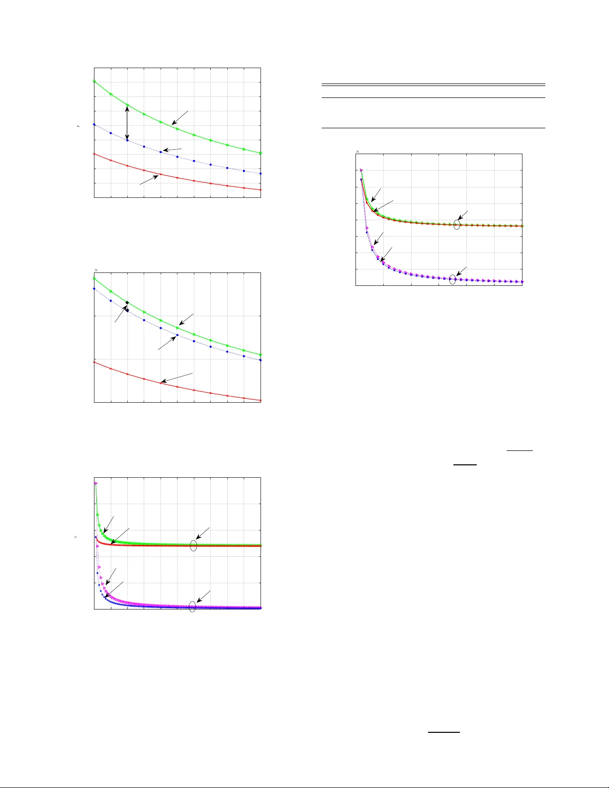
Authors: Yicheng Chen, Rick S. Blum
1 On the Impact of Unkno wn Signals in P assi ve Radar with Direct P ath and Reflected Path Observ ations Y icheng Chen, Student Member , IEEE , and Rick S. Blum, F ellow , IEEE Abstract —W e derive the closed form Cramer-Rao bound (CRB) expressions for joint estimation of time delay and Doppler shift with unknown signals with possibly known structure. The results are especially useful for passive radar where direct path and reflected path signals ar e present. T ime delay and Doppler shift estimation is an important fundamental tool in signal processing which has r eceived extensi ve study for cases with known transmitted signals, but little study f or unknown transmitted signals. The presented results generalize previous results for known transmitted signals and show how many looks from the dir ect path and the reflected path we need to deriv e an accurate joint estimation of time delay and Doppler shift. After analysis under a simple common signal-to-clutter -plus-noise ratio (SCNR) model with separated dir ect and reflected path signals, white clutter-plus-noise and line of sight propagation, extensions to cases with di ff erent direct and reflected path SCNRs, correlated clutter-plus-noise, nonseparated direct and reflected path signals and multipath pr opagation are discussed to support the utility of the CRB with unknown signals. Index T erms —Cramer -Rao bound, joint estimation, unknown signals, passive radar . I. I ntroduction The topic of time delay and Doppler shift estimation con- tinues to attract attention [1 – 15], since it is recognized to be a basic problem of significant interest in radar , communications and related sensor signal processing systems. Early work has built the foundation for four decades of research on time delay and Doppler shift estimation, see for example [16 – 20]. The recent increased attention on passive radar systems is noticeable [13, 21 – 29]. W e attribute this to several adv antages, including smaller size, less detectable radar operation, more portability and lower cost over traditional radar systems, referred to as active radar systems. An informati ve way to ev aluate the estimation performance in a radar system is to employ an achiev able lo wer bound on the estimation error . The Cramer -Rao bound (CRB) is a widely used lower bound on the variance (or mean square error) of all unbiased estimators which is achie vable using maximum likelihood estimators under mild conditions. The CRB is regarded as an important benchmark of performance in radar systems [14, 20, 30 – 32]. The CRB for estimating the time delay and Doppler shift of the target in passi ve radar systems has been calculated in [14, 30–32] under the assumption that the transmitted signal can be perfectly estimated, so the transmitted signal is assumed known. Ho wev er, in practice, the The work of Y icheng Chen and R. S. Blum was supported by the National Science Foundation under Grant No. ECCS-1405579. This material is based upon work partially supported by the U. S. Army Research Laboratory and the U. S. Army Research O ffi ce under grant number W911NF-17-1-0331. Y icheng Chen and R. S. Blum are with Lehigh University , Bethlehem, P A 18015 USA (email: yic917@lehigh.edu, rblum@eecs.lehigh.edu). exact transmitted signals from non-cooperativ e illuminators of opportunity in passive radar system are typically unknown by the passive radar system which is a topic that has not seen much in vestigation for estimation of target parameters. The impact of unknown signals on passiv e radar perfor- mance is of critical importance. In practice we typically hav e both direct path and reflected path observations ov er certain time periods, and the direct path delay and Doppler may be known or previously estimated such that it can be remov ed. Thus a canonical problem is to estimate the parameters from both a delayed and Doppler shifted version of the signal along with a zero delayed and zero Doppler shifted version of the signal. The zero delayed and zero Doppler shifted version of the signal comes from the direct path, while the delayed and Doppler shifted version of the signal comes from the reflected path. In di ff erent systems, the direct and reflected path may be separated by antenna array processing. Further in some cases, we get multiple looks at both the direct path and the reflected path signals and we would like to know how these multiple looks impact our performance, along with all the other parameters. The multiple looks could come from observations from closely spaced antenna array elements which see di ff erent noise observ ations but similar signals, delays and Doppler frequencies. While other bounds can be employed, the CRB seems to be the simplest and most studied lo wer bound. Thus, using the CRB seems a proper first step in this relativ ely unstudied direction that attempts to ev aluate parameter estimation performance with unknown signals with either unknown or known structure. Kno wing the relationship between the CRBs with unknown and known signals allo ws designers to understand the loss and decide if they should increase the number of looks or modify something else to close this gap. W e also consider the impact of knowing the signal structure which is also very important and can often be exploited in passiv e radar . W e found only one recent paper [33] which considered the performance of time delay estimation with unknown deter - ministic signals. While [33] is an interesting and useful paper, the Zi v-Zakai bound is employed in [33] after an unjustified replacement of the likelihood ratio test required by the Ziv- Zakai bound with a generalized likelihood ratio test. This modification destroys the validity of the Ziv-Zakai bound such that it is no longer known to be a bound or to have any kno wn relationship to the actual estimation performance so that the provided results are not guaranteed to be meaningful. Further , [33] does not provide simple closed-form expressions, other than those inv olving a very comp licated integral which almost always requires numerical e valuation, which limits insight. 2 W e, howe ver , provide justified bounds 1 and simple closed- form expressions which are not av ailable in [33]. In this paper , we consider the impact of unknown signals in passiv e radar with direct path and reflected path observations, but we employ canonical models, with the hope that these results might be adopted in other applications with unknown signals. W e deriv e a closed-form expression for the CRB for joint time delay and Doppler shift estimation for cases with un- known signals with either unknown or kno wn signal structure and possibly multiple looks at the direct path and reflected path returns. W e explicitly consider known structure signals consisting of amplitude modulated pulse trains. After the main analysis is described for a simple model, we discuss e xtensions to more complicated models. The main contributions of this paper are: 1. For the case of unknown signal structure and a simplified model, closed-form expressions of the Fisher information matrix (FIM) and the CRB for joint time delay and Doppler shift estimation with unknown signals are derived based on possible multiple looks at the direct path and reflected path returns. The relationship between the unknown signals CRB and the known signals CRB is obtained. It is sho wn that the unknown signals CRBs for delay and Doppler shift are each the product of the corresponding known signal CRB multiplied by a simple factor that depends on the number of looks. With a single look from the reflected path, which includes the delay and Doppler shift, and a su ffi ciently large number of looks at the direct path, which does not include the delay and Doppler shift, the CRB for unknown signals approaches that for known signals. Thus, the observations can be used to accurately estimate the unknown signal. Further , for a su ffi ciently large number of looks at both the direct and reflected paths, the CRBs can be driv en to zero. 2. Similar expressions are provided for the case where the signal has some known structure such that it can be described by some known expressions with some unkno wn parameters representing information embedded into the signals. A specific case using amplitude modulation is used to make these ideas concrete. The estimation performance is shown to improv e when the kno wn structure is acknowledged. 3. Extensions to more complicated models with di ff erent direct and reflected path SCNRs, correlated clutter-plus-noise, nonseparated direct and reflected path signals, and multipath returns are described and detailed solutions are provided or outlined. The paper is organized as follows. Joint time delay and Doppler shift estimation with known signals is discussed in Section II. The closed-form expressions of the CRB for joint time delay and Doppler shift estimation with unknown signals are de veloped in Section III. In Section IV , we derive the closed-form expressions of the CRB for joint estimation with known signal structure. Numerical examples provide the CRB for joint estimation with unknown signals with either unknown or kno wn structure in Section V . In Section VI, extensions to the observation model are considered. Finally , Section VII 1 Achiev able by maximum likelihood estimator with a su ffi cient number of obsev ations. concludes the paper . Throughout this paper, the notation for transpose is T , while the symbol | | denotes the norm. Bold lower case letters are used to denote column vectors, and bold upper case letters denote matrices. Let A i , j denote the element in the i -th row and j -th column of the matrix A , 1 denote an identity matrix and 0 denote the all zero matrix. E denotes the expectation operator . T r ( · ) denotes the trace of a matrix, ⊗ represents the Kronecker product, and vec( · ) denotes the vectorizing operator which stacks the columns of a matrix in a column vector . II. J oint estima tion with a known signal Consider the reflected path signal with unknown time delay τ 0 and Doppler shift f 0 for a completely known finite support narrow-band complex baseband transmitted signal s ( t ). Sup- pose we take discrete-time samples with a reasonably small ∆ to obtain the baseband observations x ( n ∆ ) = s ( n ∆ − τ 0 ) e j 2 π f 0 n ∆ + w ( n ∆ ) (1) for n = 0 , 1 , . . . , N − 1 with τ 0 = n 0 ∆ . If s ( n ∆ ) is zero for n < 0 and n > ( M − 1) ∆ , then x ( n ∆ ) = w ( n ∆ ) if 0 ≤ n ≤ n 0 − 1 s ( n ∆ − τ 0 ) e j 2 π f 0 n ∆ + w ( n ∆ ) if n 0 ≤ n ≤ n 0 + M − 1 w ( n ∆ ) if n 0 + M ≤ n ≤ N − 1 . The observ ations in (1) are often called the reflected-path observations in passi ve radar and they can be obtained by pointing a directional antenna in the tar get direction. Assuming independent and identically distributed (iid) complex Gaus- sian zero mean and v ariance σ 2 w clutter-plus-noise samples w ( n ∆ ) , n = 0 , . . . , N − 1, then we use the JCRB to denote the CRB for any unbiased (zero mean) joint time delay and Doppler shift estimation ( ˆ τ 0 , ˆ f 0 ) based on the observations ( x (0) , x ( ∆ ) , . . . , x (( N − 1) ∆ ) T which implies (see Appendix A) var ( ˆ τ 0 ) ≥ JC R B τ 0 = σ 2 w M − 1 P n = 0 ( t + τ 0 ) 2 | s ( t ) | 2 t = n ∆ 2 M − 1 P n = 0 ∂ s ( t ) ∂ t 2 t = n ∆ M − 1 P n = 0 ( t + τ 0 ) 2 | s ( t ) | 2 t = n ∆ − η 2 ! (2) and var ( ˆ f 0 ) ≥ JC R B f 0 = σ 2 w M − 1 P n = 0 ∂ s ( t ) ∂ t 2 t = n ∆ 8 π 2 M − 1 P n = 0 ∂ s ( t ) ∂ t 2 t = n ∆ M − 1 P n = 0 ( t + τ 0 ) 2 | s ( t ) | 2 t = n ∆ − η 2 ! (3) where η is defined as η = M − 1 X n = 0 ( t + τ 0 )( s I ( t ) ∂ s R ( t ) ∂ t − s R ( t ) ∂ s I ( t ) ∂ t ) t = n ∆ (4) and s R ( t ), s I ( t ) are the real and imaginary parts of s ( t ) respectiv ely . W e hav e treated τ 0 as a continuous variable for con venience, b ut this is a reasonable approximation for su ffi ciently fast sampling [34]. 3 III. J oint estima tion with unknown signals Now assume that s ( t ) is an unknown function of t to model the case where the narrow-band transmitted signal is unknown. This is a problem of interest for passiv e radar . Under the same high sampling rate assumptions so that the approximation of continuous time delay τ 0 is su ffi ciently accurate, then we can characterize the losses from not kno w- ing the signal by calculating the CRB for joint estimation of the components of the parameters of the vector θ = ( τ 0 , f 0 , s R (0) , s I (0) , s R ( ∆ ) , . . . , s I (( M − 1) ∆ ) T . As common in passiv e rada r , some direct path observations can be obtained by pointing directional antennas at the transmitter [21] and removing a known time delay . Let us assume that we augment the observ ations from the reflected path in (1) with x d ` ( n ∆ ) = s ( n ∆ ) + w d ` ( n ∆ ) (5) for n = 0 , 1 , . . . , N − 1 , ` = 1 , . . . , L , which we call reference observations, to help us estimate the signal samples. W e call the case without reference observ ations the L = 0 case. Assum- ing L > 0, then the observations in (5) provide L extra looks at the undelayed and nonshifted signals. Note that combining (1) with (5) together, we obtain L looks at the zero delayed and zero Doppler shifted version of the signal and one look at the delayed and Doppler shifted version of the signal. All complex clutter-plus-noise samples in (1) and (5) form an iid sequence (same model as w in (1)), and the real and imaginary parts of the signal samples s R (0) , s I (0) , s R ( ∆ ) , . . . , s I (( M − 1) ∆ ) are assumed to be deterministic unknowns. A. Generalization of the Model Suppose we generalize the model such that we get P ≥ 1 looks at the delayed and Doppler shifted signal as opposed to the P = 1 case in (1). Then we replace (1) with x r ` ( n ∆ ) = s ( n ∆ − τ 0 ) e j 2 π f 0 n ∆ + w r ` ( n ∆ ) (6) for n = 0 , . . . , N − 1, ` = 1 , . . . , P , and we augment these observations with the L looks from (5). Again, all complex clutter-plus-noise samples in (6) form an iid sequence (same model as w in (1)) and the real and imaginary parts of the signal samples s R (0) , s I (0) , s R ( ∆ ) , . . . , s I (( M − 1) ∆ ) are assumed to be deterministic unknowns. Note that the ( i , j )th entry of the FIM in this multiple parameter case can be computed as [34] I ( θ ) i , j = − E " ∂ 2 ln p ( x ; θ ) ∂ θ i ∂ θ j # (7) where the log of the probability density function (pdf) p ( x ; θ ) of x = ( x r 1 (0) , . . . , x r 1 (( N − 1) ∆ ) , x r 2 (0) , . . . , x r P (( N − 1) ∆ ) , x d 1 (0) , . . . , x d 1 (( N − 1) ∆ ) , x d 2 (0) , . . . , x d L (( N − 1) ∆ )) T is ln p ( x ; θ ) ∝ − 1 σ 2 w P X l = 1 N − 1 X n = 0 x rl ( n ∆ ) − s ( n ∆ − τ 0 ) e j 2 π f 0 n ∆ 2 + L X l = 1 N − 1 X n = 0 x dl ( n ∆ ) − s ( n ∆ ) 2 ! . (8) The FIM for estimating θ in this case is defined as I ( θ ) = " A B B T C # (9) where the specific entries in the 2 × 2 symmetric matrix A in (9) are A 1 , 1 = − E [ ∂ 2 ln p ( x ; θ ) ∂τ 2 0 ] = 2 P σ 2 w M − 1 X n = 0 ∂ s ( t ) ∂ t 2 t = n ∆ , (10) A 2 , 2 = − E [ ∂ 2 ln p ( x ; θ ) ∂ f 2 0 ] = P 8 π 2 σ 2 w M − 1 X n = 0 ( t + τ 0 ) 2 | s ( t ) | 2 t = n ∆ , (11) and A 1 , 2 = A 2 , 1 = − E [ ∂ 2 ln p ( x ; θ ) ∂τ 0 ∂ f 0 ] = 4 π P σ 2 w η (12) where η is defined in (4). The specific entries in the 2 × 2 M matrix B in (9) are B 1 , j = − E [ ∂ 2 ln p ( x ; θ ) ∂ s R ( n ∆ ) ∂τ 0 ] = − 2 P σ 2 w ∂ s R ( t ) ∂ t t = n ∆ if j = 2 n + 1 − E [ ∂ 2 ln p ( x ; θ ) ∂ s I ( n ∆ ) ∂τ 0 ] = − 2 P σ 2 w ∂ s I ( t ) ∂ t t = n ∆ if j = 2 n + 2 , (13) and B 2 , j = − E [ ∂ 2 ln p ( x ; θ ) ∂ s R ( n ∆ ) ∂ f 0 ] = − 4 π P ( t + τ 0 ) s I ( t ) σ 2 w t = n ∆ if j = 2 n + 1 − E [ ∂ 2 ln p ( x ; θ ) ∂ s I ( n ∆ ) ∂ f 0 ] = 4 π P ( t + τ 0 ) s R ( t ) σ 2 w t = n ∆ if j = 2 n + 2 , (14) for n = 0 , . . . , M − 1. The specific entries in the 2 M × 2 M diagonal matrix C in (9) are C j , j = 2 L + 2 P σ 2 w if j = 1 , 2 , ..., 2 M . (15) The Schur complement relation [35] has been used to deri ve [ I ( θ ) − 1 ] ( { 1 , 2 } , { 1 , 2 } ) = ( A − B C − 1 B T ) − 1 (16) where [ I ( θ ) − 1 ] ( { 1 , 2 } , { 1 , 2 } ) denotes the sub-matrix of I ( θ ) − 1 which consists of the elements located in the first two ro ws and the first two columns. Using the expressions of elements in A , B and C deriv ed in (10)–(15), we obtain A − B C − 1 B T = LP L + P 2 σ 2 w M − 1 P n = 0 ∂ s ( t ) ∂ t 2 t = n ∆ 4 πη σ 2 w LP L + P 4 πη σ 2 w LP L + P LP L + P 8 π 2 σ 2 w M − 1 P n = 0 ( t + τ 0 ) 2 | s ( t ) | 2 t = n ∆ (17) where η is defined in (4). Any unbiased joint estimate of time delay , Doppler shift and signal samples satisfies [34] var( ˆ τ 0 ) ≥ JC R B τ 0 , s (18) where [35] JC R B τ 0 , s = h I ( θ ) − 1 i 1 , 1 = h ( A − B C − 1 B T ) − 1 i 1 , 1 = " ad j ( A − B C − 1 B T ) d et ( A − B C − 1 B T ) # 1 , 1 = L P L + P 8 π 2 σ 2 w M − 1 X n = 0 ( t + τ 0 ) 2 | s ( t ) | 2 t = n ∆ · 1 LP L + P 8 π 2 σ 2 w M − 1 P n = 0 ( t + τ 0 ) 2 | s ( t ) | 2 t = n ∆ LP L + P 2 σ 2 w M − 1 P n = 0 ∂ s ( t ) ∂ t 2 t = n ∆ − 4 πη σ 2 w LP L + P 2 4 = L + P L P · σ 2 w 2 M − 1 P n = 0 ( t + τ 0 ) 2 | s ( t ) | 2 t = n ∆ M − 1 P n = 0 ∂ s ( t ) ∂ t 2 t = n ∆ M − 1 P n = 0 ( t + τ 0 ) 2 | s ( t ) | 2 t = n ∆ − η 2 = L + P L P JC R B τ 0 (19) where (2) is employed and η is defined in (4). Similarly , any unbiased joint estimate of time delay , Doppler shift and signal samples satisfies [34] var( ˆ f 0 ) ≥ = JC R B f 0 , s (20) where [35] JC R B f 0 , s = h I ( θ ) − 1 i 2 , 2 = h ( A − B C − 1 B T ) − 1 i 2 , 2 = " ad j ( A − B C − 1 B T ) d et ( A − B C − 1 B T ) # 2 , 2 = L P L + P 2 σ 2 w M − 1 X n = 0 ∂ s ( t ) ∂ t 2 t = n ∆ · 1 LP L + P 8 π 2 σ 2 w M − 1 P n = 0 ( t + τ 0 ) 2 | s ( t ) | 2 t = n ∆ LP L + P 2 σ 2 w M − 1 P n = 0 ∂ s ( t ) ∂ t 2 t = n ∆ − 4 πη σ 2 w LP L + P 2 = L + P L P · σ 2 w 8 π 2 M − 1 P n = 0 ∂ s ( t ) ∂ t 2 t = n ∆ M − 1 P n = 0 ∂ s ( t ) ∂ t 2 t = n ∆ M − 1 P n = 0 ( t + τ 0 ) 2 | s ( t ) | 2 t = n ∆ − η 2 = L + P L P JC R B f 0 (21) where (3) is employed and η is defined in (4). If we estimate τ 0 and f 0 separately for unknown signals, whose CRB we denote as C R B τ 0 , s and C R B f 0 , s respectiv ely, then (19) and (21) still hold. Thus, C R B τ 0 , s = L + P L P C R B τ 0 , (22) with C R B τ 0 = σ 2 w 2 M − 1 P n = 0 ∂ s ( t ) ∂ t 2 t = n ∆ , (23) and C R B f 0 , s = L + P L P C R B f 0 , (24) with C R B f 0 = σ 2 w 8 π 2 M − 1 P n = 0 ( t + τ 0 ) 2 | s ( t ) | 2 t = n ∆ . (25) For L = 0 and any finite P ≥ 1, (19) and (21) imply there is no unbiased joint estimator of the time delay τ 0 and Doppler shift f 0 . Similarly , if P = 0 with any finite L ≥ 1, (19) and (21) imply there is no unbiased joint estimator of the time delay τ 0 and Doppler shift f 0 . This is reasonable. In fact, it makes sense that we need to see at least one look at the delayed Doppler shifted and undelayed nonDoppler shifted signals to pro vide an accurate joint estimation. It is clear that JC R B τ 0 , s and J C RB f 0 , s are decreasing in either L or P . From the symmetry of (19) and (21), the e ff ect of increasing either L or P is exactly the same, as we might expect 2 . If we want to compare to the kno wn signal case, (2) and (3), we should recall we just had one look at the time delayed and Doppler shifted version of the signal in that case so it seems P = 1 should be considered to be fair . In this case (19) and (21) imply that JC R B τ 0 , s and J C RB f 0 , s are generally lar ger than JC R B τ 0 and JC R B f 0 for finite L , respecti vely . In fact the factor L + P LP | P = 1 captures the exact increase in a beautiful and simple e xpression. This is interesting since for either L = 1 or P = 1, JC R B τ 0 , s and J C R B f 0 , s approach J C R B τ 0 and JC R B f 0 respectiv ely as the other variable (number of looks) approaches infinity . If L > 1 or P > 1, then JC R B τ 0 , s and JC R B f 0 , s approach a v alue smaller than J C RB τ 0 and J C R B f 0 respectiv ely as the other variable approaches infinity . The reason is that J C R B τ 0 and J C R B f 0 are calculated with only one look. If you generalize the model in (1) to R looks, then the JCRB can easily be seen to be JC R B R . Thus the stated limits of JC R B τ 0 P and JC R B f 0 P as L increases tow ards infinity or JC R B τ 0 L and JC R B f 0 L as P increases to wards infinity should be expected. On the other hand, if L = P then by making their common value su ffi ciently large, we can make J C R B τ 0 , s and J C RB f 0 , s as close to zero as we like. This seems reasonable since in this case we can perfectly categorize both the undelayed non- Doppler shifted and the delayed Doppler shifted signal. IV . K nown signal str ucture Suppose s ( t ) is a communication signal with known struc- ture and unknown parameters containing information. For example, assume a pulse amplitude modulation signal with unknown complex pulse amplitudes b q , q = 1 , ..., Q such that s ( n ∆ ) = 0 for n < 0 and n > M − 1 and for n 0 ≤ n ≤ n 0 + M − 1 s ( n ∆ − τ 0 ) = Q X q = 1 b q g ( n ∆ − τ 0 − ( q − 1) T p ) (26) where we assume we know the pulse shape g ( t ). Further the total support of the signal is still M samples where M ∆ = QT P . In this case, we need to estimate the pulse amplitudes instead of the signal samples. Thus the parameter to estimate becomes θ = ( τ 0 , f 0 , b 1 R , b 1 I , b 2 R , b 2 I , ..., b QR , b QI ) T where b qR and b qI are the real and imagery parts of the complex pulse amplitudes b q , q = 1 , ..., Q . It should be noted that Q , the number of pulses, is smaller than the number of signal samples used if there is more than one sample per pulse, reasonable for unknown signals. Thus the estimation performance when only estimating the pulse amplitudes should be more fa vorable since we estimate fewer parameters as we show next. While we assume the pulse amplitudes can take on any complex value, the analysis gi ves a good approximation if the real and imaginary parts of pulse amplitudes are discrete with many lev els. Define h ( q ) = M − 1 X n = 0 d d t s ( t ) ! t = n ∆ g ( n ∆ − ( q − 1) T p ) ! , 2 See Section VI for di ff erent direct and reflected path channels. 5 u ( q ) = M − 1 X n = 0 ( s ( t ) ) ( t + τ 0 ) t = n ∆ g ( n ∆ − ( q − 1) T p ) ! , and c ( q , q 0 ) = M − 1 X n = 0 g ( n ∆ − ( q − 1) T p ) g ( n ∆ − ( q 0 − 1) T p ) . (27) The FIM for estimating θ in this case is I ( θ ) = " A B 0 B 0 T C 0 # (28) where the expressions of the specific elements in the 2 × 2 symmetric matrix A are giv en in (10)–(12). The specific entries in the 2 × 2 Q matrix B 0 for q = 1 , ..., Q are B 0 1 , j = − E [ ∂ 2 ln p ( x ; θ ) ∂ b R ( n ∆ ) ∂τ 0 ] = − 2 P σ 2 w h R ( q ) if j = 2 q − 1 − E [ ∂ 2 ln p ( x ; θ ) ∂ b I ( n ∆ ) ∂τ 0 ] = − 2 P σ 2 w h I ( q ) if j = 2 q , (29) and B 0 2 , j = − E [ ∂ 2 ln p ( x ; θ ) ∂ b R ( n ∆ ) ∂ f 0 ] = − 4 π P σ 2 w u I ( q ) if j = 2 q − 1 − E [ ∂ 2 ln p ( x ; θ ) ∂ b I ( n ∆ ) ∂ f 0 ] = 4 π P σ 2 w u R ( q ) if j = 2 q , (30) where h R ( q ), h I ( q ) are the real and imaginary parts of h ( q ) defined in (27), and u R ( q ), u I ( q ) are the real and imaginary parts of u ( q ) defined in (27). The entries in the 2 Q × 2 Q matrix C 0 for q , q 0 = 1 , . . . , Q are C 0 2 q − 1 , 2 q 0 − 1 = − E [ ∂ 2 ln p ( x ; θ ) ∂ b qR ∂ b q 0 R ] = 2( P + L ) σ 2 w c ( q , q 0 ) , (31) C 0 2 q , 2 q 0 = − E [ ∂ 2 ln p ( x ; θ ) ∂ b qI ∂ b q 0 I ] = 2( P + L ) σ 2 w c ( q , q 0 ) , (32) and C 0 2 q − 1 , 2 q 0 = − E [ ∂ 2 ln p ( x ; θ ) ∂ b qR ∂ b q 0 I ] = 0 . (33) W e can simplify the expressions considerably if g ( n ∆ ) is nonzero only ov er the duration of 0 < n ∆ < T P = n p ∆ , which is often a reasonable approximation. In this case, the FIM is I ( θ ) = " A B 00 B 00 T C 00 # (34) where the elements in the 2 × 2 symmetric matrix A are given in (10)–(12). The entries in the 2 × 2 Q matrix B 00 and those in the 2 Q × 2 Q diagonal matrix C 00 are B 00 = − 2 P ρ b 1 R σ 2 w − 2 P ρ b 1 I σ 2 w − 2 P ρ b 2 R σ 2 w · · · − 2 P ρ b QI σ 2 w − 4 π P γ 1 b 1 I σ 2 w 4 π P γ 1 b 1 R σ 2 w − 4 π P γ 2 b 2 I σ 2 w · · · 4 π P γ Q b QR σ 2 w , (35) and C j , j = (2 L + 2 P ) E g σ 2 w if j = 1 , 2 , ..., 2 Q (36) with ρ = n p X n = 0 d d t g ( t ) ! t = n ∆ g ( n ∆ ) ! , (37) γ q = n p X n = 0 ( n ∆ + τ 0 + ( q − 1) T P )( g ( n ∆ )) 2 , (38) and E g = n p X n = 0 ( g ( n ∆ ) ) 2 . (39) Similar to (16), by using the Schur complement relation and (34), we obtain [ I ( θ ) − 1 ] ( { 1 , 2 } , { 1 , 2 } ) = ( A − B 00 ( C 00 ) − 1 B 00 T ) − 1 (40) where [ I ( θ ) − 1 ] ( { 1 , 2 } , { 1 , 2 } ) denotes the sub-matrix of I ( θ ) − 1 which consists of the elements located in the first two rows and the first two columns and we define a 2 × 2 matrix V = ( A − B 00 ( C 00 ) − 1 B 00 T ) where V 1 , 1 = 2 P σ 2 w Q X q = 1 b q 2 n p X n = 0 ( dg ( t ) dt ) 2 t = n ∆ − P ( L + P ) ρ 2 E g Q X q = 1 b q 2 , (41) V 2 , 2 = 8 π 2 P σ 2 w Q X q = 1 ( n p X n = 0 ( t + τ 0 + ( q − 1) T p ) 2 · ( g ( t )) 2 ) t = n ∆ b q 2 − P L + P 1 E g Q X q = 1 γ 2 q b q 2 , (42) and V 2 , 1 = V 1 , 2 = A 1 , 2 − 2 Q X j = 1 B 00 1 , j h C 00− 1 i j , j B 00 T j , 2 = 4 π P σ 2 w η − σ 2 w (2 L + 2 P ) E g Q X q = 1 8 π P 2 ρ b qR σ 2 w γ q b qI σ 2 w − 8 π P 2 ρ b qI σ 2 w γ q b qR σ 2 w ! = 4 π P σ 2 w η = 4 π P σ 2 w M − 1 X n = 0 ( t + τ 0 ) Q X q = 1 b qI g ( t − ( q − 1) T p ) · Q X q = 1 b qR ∂ g ( t − ( q − 1) T p ) ∂ t − Q X q = 1 b qR g ( t − ( q − 1) T p ) · Q X q = 1 b qI ∂ g ( t − ( q − 1) T p ) ∂ t t = n ∆ = 4 π P σ 2 w M − 1 X n = 0 ( t + τ 0 ) Q X q = 1 b qI b qR g ( t − ( q − 1) T p ) · ∂ g ( t − ( q − 1) T p ) ∂ t − Q X q = 1 b qR b qI g ( t − ( q − 1) T p ) · ∂ g ( t − ( q − 1) T p ) ∂ t t = n ∆ = 0 (43) where we have used the results in (12), (35) and (36) to obtain the second line. Since the second term in the second line is zero, we obtain the third line. W e have used the kno wn signal structure to obtain the fourth line and we used the assumption that g ( n ∆ ) is nonzero only ov er the duration of 0 < n ∆ < T P = n p ∆ to obtain the fifth line. Thus when performing the joint estimation of time delay , Doppler shift and the complex pulse amplitudes var( ˆ τ 0 ) ≥ JC R B τ 0 , b (44) where J C R B τ 0 , b is calculated as JC R B τ 0 , b = [ I ( θ ) − 1 ] 1 , 1 = σ 2 w 2 P Q X q = 1 b q 2 n p X n = 0 ( d g ( t ) d t ) 2 t = n ∆ − P L + P ρ 2 E g Q X q = 1 b q 2 − 1 . (45) 6 Similar to (44), any unbiased estimate of time delay , Doppler shift and the complex pulse amplitudes together satisfies var( ˆ f 0 ) ≥ JC R B f 0 , b (46) where J C R B f 0 , b is deri ved as JC R B f 0 , b = [ I ( θ ) − 1 ] 2 , 2 = σ 2 w 8 π 2 P Q X q = 1 ( n p X n = 0 ( t + τ 0 + ( q − 1) T p ) 2 · ( g ( t )) 2 ) t = n ∆ b q 2 − P L + P 1 E g Q X q = 1 γ 2 q b q 2 − 1 . (47) For the case where g ( n ∆ ) is nonzero only ov er the duration of 0 < n ∆ < T P = n p ∆ , the JCRB of the time delay and Doppler shift estimation with known signals in (2) becomes JC R B τ 0 = σ 2 w 2 Q P q = 1 b q 2 n p P n = 0 ( dg ( t ) dt ) 2 t = n ∆ . (48) Similar to (48), the JCRB of the time delay and Doppler shift estimation with kno wn signals satisfies JC R B f 0 = σ 2 w 8 π 2 Q P q = 1 n p P n = 0 ( t + τ 0 + ( q − 1) T p ) 2 · ( g ( t )) 2 ! t = n ∆ b q 2 . (49) Provided g ( t ) is not equal to a scalar multiple of d d t g ( t ) and n p , 0 , from the Schwartz inequality , (37) and (39), we find ρ 2 < E g n p X n = 0 d d t g ( t ) ! 2 t = n ∆ . (50) For P > 0, L > 0, multiplying both sides by − P L + P · 1 E g Q P q = 1 b q 2 implies − P L + P · ρ 2 E g Q X q = 1 b q 2 > − P L + P · Q X q = 1 b q 2 n p X n = 0 ( d g ( t ) d t ) 2 t = n ∆ . (51) Adding Q P q = 1 b q 2 n p P n = 0 ( dg ( t ) dt ) 2 t = n ∆ to both sides yields, Q P q = 1 b q 2 n p P n = 0 ( dg ( t ) dt ) 2 t = n ∆ − P L + P · ρ 2 E g Q P q = 1 b q 2 > Q P q = 1 b q 2 n p P n = 0 ( dg ( t ) dt ) 2 t = n ∆ − P L + P · Q P q = 1 b q 2 n p P n = 0 ( dg ( t ) dt ) 2 t = n ∆ . (52) Calculating the reciprocal of both sides of (52) and multiplying both sides of them by σ 2 w 2 P implies σ 2 w 2 P · Q P q = 1 b q 2 n p P n = 0 ( dg ( t ) dt ) 2 t = n ∆ − P L + P · ρ 2 E g Q P q = 1 b q 2 ! − 1 < σ 2 w 2 P · Q P q = 1 b q 2 n p P n = 0 ( dg ( t ) dt ) 2 t = n ∆ − P L + P · Q P q = 1 b q 2 n p P n = 0 ( dg ( t ) dt ) 2 t = n ∆ ! − 1 . (53) According to (45), the left side of (53) is J C R B τ 0 , b . Using (48), the right side of (53) is L + P LP JC R B τ 0 . This implies (giv en bold above (50)) J C RB τ 0 , b < J C R B τ 0 , s from previous results in (19). Similarly , we can sho w J C R B f 0 , b < J C R B f 0 , s . Thus, the known signal structure will help to improv e the estimation performance compared with that from totally unkno wn signals. Noting that P = 2 P 2 ρ 2 P Q q = 1 | b q | 2 ( L + P ) E g ≥ 0 and that JC RB τ 0 , b in (45) is monotonic increasing in P for ev erything else constant, then the smallest possible J C R B τ 0 , b occurs when P = 0. Interestingly , from (37), ρ can be zero for symmetric pulse wa veforms so such waveforms can produce this smallest pos- sible J C R B τ 0 , b . In the numerical example section, numerical results will show the magnitude of the performance gains for the known signal structure in (45) and (47) over totally unknown signals. If we estimate τ 0 and f 0 separately instead of jointly , we can sho w C RB τ 0 , b < C R B τ 0 , s and C R B f 0 , b < C R B f 0 , s where we can show C R B τ 0 , b = J C R B τ 0 , b and C R B f 0 , b = J C R B f 0 , b since we hav e shown V 2 , 1 = V 1 , 2 = 0 in (43). V . N umerical E xamples Initially consider the case where the transmitted signal s ( t ) is completely unknown to the estimator but is described by (26) for b 2 qR = b 2 qI = + 1 for q = 1 , . . . , Q (one of many possible examples). Assume the case where g ( n ∆ ) is nonzero only over the duration of 0 < n ∆ < T p = n p ∆ where n p ∆ = T p = 4 , n p = 10 , 11 , ..., 20. In particular g ( n ∆ ) = exp ( − ( n ∆ − 4) 2 / 9) for n = 0 , . . . , n p and zero elsewhere. Let P = L = 1, τ 0 = 0 . 5, σ 2 w = 0 . 1, Q = 1 and M = Qn p . As a function of n p , the number of samples per pulse, JC R B τ 0 , JC R B τ 0 , s and JC R B τ 0 , b of the joint estimation are shown in Fig. 1. Similar numerical results for JC R B f 0 , J C R B f 0 , s and JC R B f 0 , b are sho wn in Fig. 2. These results illustrate the gains of the joint estimation with known signal structure when compared with totally unknown signals. It is worth noting that the case just considered employed a nearly symmetric pulse communication signal, as might typically be exploited in passiv e radar, which produces a small ρ in (37). On the other hand γ q in (38) can not be zero so that Fig. 1 and Fig. 2 show di ff erent sized gains between the unknown signals JCRB and the known format JCRB due to the di ff erent impact of the second term inside the () − 1 in (45) and (47). For di ff erent signals, the results might be di ff erent. Consider the same signal example but let ∆ = 0 . 01, n p = 500, τ 0 = 0 . 05, f 0 = 20, Q = 2, M = Qn p and σ 2 w = 1. For P = 1 with e xpressions in (19) and (21), we find J C R B τ 0 , J C RB τ 0 , s , JC R B f 0 and J C R B f 0 , s as shown in T able I. This indicates that JC R B τ 0 , s , J C R B f 0 , s approach J C R B τ 0 , J C R B f 0 respectiv ely for large L and P = 1 as expected. This is also shown in the top curve in Fig. 3 and Fig. 4 which is labeled "unkno wn signal P = 1" for the time delay and Doppler shift, respectively . The results for di ff erent σ 2 w look very similar to the results in T able I, Fig. 3 and Fig. 4 with the only di ff erence being the σ 2 w dependence in (2) and (3) which scales the results. If we increase both P and L together we can make J C RB τ 0 , s smaller than J C R B τ 0 as e xpected and for lar ge P = L , J C R B τ 0 , s approaches zero as sho wn in the second lowest curve in Fig. 3 7 10 11 12 13 14 15 16 17 18 19 20 n p 0.02 0.03 0.04 0.05 0.06 0.07 0.08 0.09 0.1 0.11 JCRB 0 gains unknown signal known signal known format Fig. 1. J C R B τ 0 , JC RB τ 0 , s and JC RB τ 0 , b of the joint estimation for increasing samples n p when P = L = 1. 10 11 12 13 14 15 16 17 18 19 20 n p 0.5 1 1.5 2 JCRB f 0 10 -5 gains unknown signal known format known signal Fig. 2. JC RB f 0 , J C R B f 0 , s and J C R B f 0 , b of the joint estimation for increasing samples n p when P = L = 1. 0 10 20 30 40 50 60 70 80 90 100 L 0 0.005 0.01 0.015 0.02 0.025 JCRB 0 unknown signal unknown signal P=1 P=L known format known format Fig. 3. As L increases, both the unknown signal JC R B τ 0 , s (unknown form) and the known signal format J C RB τ 0 , b con verge to the known signal JC RB τ 0 when P = 1 and to zero when P = L . which is labeled "unknown signal P = L ". It is similar for the Doppler shift case which is shown in Fig. 4. Consider the same parameters as for the unknown signals case but no w assume only the pulse amplitudes b q , the time delay τ 0 and the Doppler shift f 0 are unkno wn as in Section IV. T ABLE I T he CRB s with U nknown and K nown S ignals R esul ts L JC RB τ 0 , s JC RB τ 0 JC RB f 0 , s (10 − 5 ) J C R B f 0 (10 − 5 ) 1 0.0239 0.0119 0.3506 0.1753 2 0.0179 0.0119 0.2629 0.1753 100 0.0121 0.0119 0.1770 0.1753 0 5 10 15 20 25 30 L 0 0.5 1 1.5 2 2.5 3 3.5 4 JCRB f0 10 -6 unknown signal known format unknown signal known format P=1 P=L Fig. 4. As L increases, both the unknown signal J C R B f 0 , s (unknown form) and the known signal format J C R B f 0 , b con verge to the known signal JC RB f 0 when P = 1 and to zero when P = L . The second highest curve in Fig. 3, labeled "known format P = 1" shows the advantages of knowing the signal format (compared to the highest) and estimating the pulse amplitudes rather than the samples. This implies we estimate a factor of n p = 500 fewer unknowns. The lowest curve in Fig. 3, labeled "known format P = L " shows the advantages of knowing the signal format when P = L . The adv antage for large P = L is clear if we compare (19), which decays as 2 JC RB τ 0 L when P = L , to (45), which decays as JC R B τ 0 L with a small ρ for large P = L . Similar results for JC R B f 0 are sho wn in Fig. 4. VI. E xtensions After analysis with the basic models in (5) and (6) for un- known signals and extensions to signals with known structure, further extensions are studied in this section. A. Di ff erent Known and Unknown SCNR for the Dir ect and Reflected P aths First consider the case where the reflected path model is di ff erent from the model in (6), so that the reflected path signal is x r ` ( n ∆ ) = a s ( n ∆ − τ 0 ) e j 2 π f 0 n ∆ + w r ` ( n ∆ ) (54) for n = 0 , . . . , N − 1 and ` = 1 , . . . , P , where a is a known factor which characterizes the di ff erent SCNR of the reflected path when compared to the direct path. The SCNR is scaled by the factor a if the variance σ 2 w of the clutter-plus-noise is exactly the same as we used in (5) and (6). If we repeat the calculations in Section III and Section IV , the previous results should be modified to JC R B τ 0 , s = L + a 2 P L P JC R B τ 0 (55) 8 with a redefined J C R B τ 0 JC R B τ 0 = σ 2 w M − 1 P n = 0 ( t + τ 0 ) 2 | s ( t ) | 2 t = n ∆ 2 a 2 M − 1 P n = 0 ∂ s ( t ) ∂ t 2 t = n ∆ M − 1 P n = 0 ( t + τ 0 ) 2 | s ( t ) | 2 t = n ∆ − η 2 ! . (56) Further , JC R B f 0 , s = L + a 2 P L P JC R B f 0 (57) with a redefined J C R B f 0 JC R B f 0 = σ 2 w M − 1 P n = 0 ∂ s ( t ) ∂ t 2 t = n ∆ 8 π 2 a 2 M − 1 P n = 0 ∂ s ( t ) ∂ t 2 t = n ∆ M − 1 P n = 0 ( t + τ 0 ) 2 | s ( t ) | 2 t = n ∆ − η 2 ! . (58) Further , we can again show J C RB τ 0 , b < JC R B τ 0 , s and JC R B f 0 , b < J C RB f 0 , s . If τ 0 and f 0 are estimated separately for unknown signals with the known factor a , C RB τ 0 , b < C R B τ 0 , s and C R B f 0 , b < C R B f 0 , s can also be shown and the results in (22) and (24) become C R B τ 0 , s = L + a 2 P L P C R B τ 0 (59) with C R B τ 0 = σ 2 w 2 a 2 M − 1 P n = 0 ∂ s ( t ) ∂ t 2 t = n ∆ , (60) and C R B f 0 , s = L + a 2 P L P C R B f 0 (61) with C R B f 0 = σ 2 w 8 π 2 a 2 M − 1 P n = 0 ( t + τ 0 ) 2 | s ( t ) | 2 t = n ∆ . (62) This makes sense since the relativ e importance of the obser- vations from (5) and (54) are di ff erent due to the di ff erent SCNRs. If the factor a is unknown and needs to be estimated with the other unknowns, we still obtain (55) (57) (59) (61) and sho w J C RB τ 0 , b < JC R B τ 0 , s , J C R B f 0 , b < JC R B f 0 , s , C R B τ 0 , b < C R B τ 0 , s and C RB f 0 , b < C R B f 0 , s where JC R B τ 0 , b = σ 2 w 2 a 2 P Q P q = 1 b q 2 E g E g n p P n = 0 dg ( t ) dt 2 t = n ∆ − ρ 2 , (63) JC R B f 0 , b = σ 2 w 8 π 2 a 2 P Q X q = 1 ( n p X n = 0 ( t + τ 0 + ( q − 1) T p ) 2 · ( g ( t )) 2 ) t = n ∆ b q 2 − a 2 P L + a 2 P 1 E g Q X q = 1 γ 2 q b q 2 − 1 , (64) C R B τ 0 , b = σ 2 w 2 a 2 P Q P q = 1 b q 2 E g E g n p P n = 0 dg ( t ) dt 2 t = n ∆ − ρ 2 , (65) and C R B f 0 , b = σ 2 w 8 π 2 a 2 P Q X q = 1 ( n p X n = 0 ( t + τ 0 + ( q − 1) T p ) 2 · ( g ( t )) 2 ) t = n ∆ b q 2 − a 2 P L + a 2 P 1 E g Q X q = 1 γ 2 q b q 2 − 1 . (66) The proof is provided in Appendix B and it should be noted that C R B τ 0 , b = J C R B τ 0 , b and C R B f 0 , b = J C R B f 0 , b which are also sho wn in Appendix B. B. Correlated Clutter-Plus-Noise The observations from the direct path in (5) at the l -th look can be collected in a vector as x dl = [ x dl (0) , x dl ( ∆ ) , ..., x dl (( N − 1) ∆ )] T = s 0 + w dl (67) where the N × 1 transmitted signal vector s 0 is s 0 = [ s (0) , s ( ∆ ) , ..., s (( M − 1) ∆ ) , 0 , ..., 0] T , (68) and the N × 1 noise vector w dl at the l -th look is w dl = [ w dl (0) , w dl ( ∆ ) , ..., w dl (( N − 1) ∆ )] T . (69) Similarly , the observations from the reflected path in (6) at the l -th look can be collected in a vector as x rl = [ x rl (0) , x rl ( ∆ ) , ..., x rl (( N − 1) ∆ )] T = s τ 0 f 0 + w rl (70) where the N × 1 transmitted signal vector s τ 0 f 0 is s τ 0 f 0 = [0 , ..., 0 , s (0) e j 2 π f 0 n 0 ∆ , s ( ∆ ) e j 2 π f 0 ( n 0 + 1) ∆ , ..., s (( M − 1) ∆ ) e j 2 π f 0 ( n 0 + M − 1) ∆ , 0 , ..., 0] T , (71) and the N × 1 noise vector w rl at the l -th look is w rl = [ w rl (0) , w rl ( ∆ ) , ..., w rl (( N − 1) ∆ )] T . (72) The observations from the direct path and reflected path can be written as x = [ x T d 1 , x T d 2 , ..., x T d L , x T r 1 , x T r 2 , ..., x T r P ] T = s + w (73) where the signal vector s is s = [ s T 0 , s T 0 , ..., s T 0 , s T τ 0 f 0 , s T τ 0 f 0 , ..., s T τ 0 f 0 ] T , (74) and the clutter -plus-noise vector w is w = [ w T d 1 , w T d 2 , ..., w T d L , w T r 1 , w T r 2 , ..., w T r P ] T (75) which is assumed to be complex Gaussian distributed with zero mean and cov ariance matrix Q = E { ww H } . Note that this models either the a = 1 case or the a , 1 case since the a , 1 case in (54) can be represented as the case in (70) with a reduction in the noise variance by 1 a 2 . So the a , 1 case can be handled by modifying Q . Since we gi ve the results for arbitrary Q , we already consider the a , 1 case. 9 Using the receiv ed signal model previously described but now assuming correlated Gaussian clutter-plus-noise, the pdf of the observ ation vector is p ( x | θ ) = 1 π N ( P + L ) det( C ) exp( − x H C − 1 x ) (76) with the cov ariance matrix C is C = E n ( s + w ) ( s + w ) H o = E n ss H + ww H o = E { ss H } + Q . (77) The ( i , j )th element of the FIM for the parameter vector θ = ( τ 0 , f 0 , s R (0) , s I (0) , s R ( ∆ ) , . . . , s I ( ∆ ( M − 1)) T is given by [34] [ I ( θ ) ] i , j = T r C − 1 ∂ C ∂θ i C − 1 ∂ C ∂θ j ! . (78) W e can rewrite (78) as [36] [ I ( θ ) ] i , j = T r ∂ C ∂θ i C − 1 ∂ C ∂θ j C − 1 ! = ∂ C vec ∂θ i ! H C −† ⊗ C − 1 ∂ C vec ∂θ j ! (79) where C vec = vec ( C ) . Then the FIM for estimating θ is I ( θ ) = J τ 0 τ 0 J τ 0 f 0 J τ 0 s a J τ 0 f 0 J f 0 f 0 J f 0 s a J s a τ 0 J s a f 0 J s a s a (80) where J τ 0 τ 0 = J H τ 0 J τ 0 , J τ 0 f 0 = J H f 0 τ 0 = J H τ 0 J f 0 , J τ 0 s a = J H s a τ 0 = J H τ 0 J s a , J f 0 f 0 = J H f 0 J f 0 , J f 0 s a = J H s a f 0 = J H f 0 J s a , J s a s a = J H s a J s a , J τ 0 = C −† / 2 ⊗ C − 1 / 2 ∂ C vec ∂τ 0 , (81) J f 0 = C −† / 2 ⊗ C − 1 / 2 ∂ C vec ∂ f 0 , (82) and J sa = C −† / 2 ⊗ C − 1 / 2 ∂ C vec ∂ s a T (83) with s a = [ s R (0) , s I (0) , s R ( ∆ ) , ..., s I (( M − 1) ∆ )] T . (84) Giv en any unbiased estimator ˆ θ of an unknown parameter vector θ based on an observation vector x , we hav e [34] MSE = E n ( ˆ θ − θ )( ˆ θ − θ ) T o JCRB( θ ) = I − 1 ( θ ) . (85) One could calculate the closed form JCRB with unkno wn signals in correlated Gaussian clutter-plus-noise by using the results from (77), (80)–(84). C. Nonseparated Dir ect P ath and Reflected P ath In order to simplify our analysis, we only consider real signals and time delay estimation. The receiv ed signals with nonseparated direct and reflected path can be represented as x l ( n ∆ ) = s ( n ∆ ) + s ( n ∆ − τ 0 ) + w l ( n ∆ ) (86) for n = 0 , 1 , ..., N − 1 and l = 1 , ..., P where s ( n ∆ ) is nonzero only during the duration 0 < n < M − 1, and Fig. 5. A diagram showing the signals from the direct path and the reflected path returns without overlap in time domain. s ( n ∆ − τ 0 ) is nonzero only during the duration n 0 < n < n 0 + M − 1. The w l ( n ∆ ) , n = 0 , 1 , ..., N − 1 are real clutter- plus-noise samples with variance σ 2 w and P is the number of looks at the signal. The unknown parameter vector is θ = ( τ 0 , s (0) , s ( ∆ ) , . . . , s (( M − 1) ∆ )) T and the likelihood function of x = ( x 10 , . . . , x 1( N − 1) , x 20 , . . . , x P ( N − 1) ) T is p ( x ; θ ) ∝ exp {− 1 2 σ 2 w P X l = 1 N − 1 X n = 0 ( x l [ n ] − s ( n ∆ ) − s ( n ∆ − τ 0 )) 2 } (87) In the follo wing, the transmitted signal length M is fixed and the impact of overlap on the CRB is in vestigated by changing the value of n 0 . When the two signals from the direct path and reflected path returns do not overlap in time, it implies n 0 > M − 1, see Fig. 5. Let e be a scalar , b be a M × 1 column vector and D be a M × M matrix. Now the FIM for estimating θ is I ( θ ) = " e b T b D # (88) with e = − E [ ∂ 2 ln p ( x ; θ ) ∂τ 2 0 ] = P σ 2 w M − 1 X n = 0 ( ∂ s ( t ) ∂ t ) 2 t = n ∆ , (89) b j = − E [ ∂ 2 ln p ( x ; θ ) ∂τ 0 ∂ s ( n ∆ ) ] = − P σ 2 w ∂ s ( t ) ∂ t t = n ∆ if j = n + 1 , (90) D j , j = − E [ ∂ 2 ln p ( x ; θ ) ∂ s ( n ∆ ) ∂ s ( n ∆ ) ] = 2 P σ 2 w if j = n + 1 , (91) for n = 0 , . . . , M − 1 and the other FIM entries, not mentioned, are all zero. The CRB with nonoverlapped signals satisfies C R B τ 0 , non = [ I ( θ ) ] − 1 11 = e − M X j = 1 b j D − 1 j , j b j − 1 = 2 P P 2 σ 2 w M − 1 P n = 0 d s ( t ) dt 2 t = n ∆ (92) which follo ws, as e xpected, the previous results we gav e before when we set L = P but no w we only estimate the time delay and signal samples without Doppler shift estimation. When the two signals from the direct path and reflected path returns are overlapped in time, it implies 0 ≤ n 0 ≤ M − 1, see Fig. 6. When these two signals are totally overlapped, which im- plies n 0 = 0. Let e be a scalar defined in (89), b 0 be a M × 1 column vector and D 0 be a M × M matrix. The FIM for estimating θ becomes I ( θ ) = " e b 0 T b 0 D 0 # (93) 10 Fig. 6. A diagram showing the signals from the direct path and the reflected path returns with overlap in time domain. with b 0 j = − E [ ∂ 2 ln p ( x ; θ ) ∂τ 0 ∂ s ( n ∆ ) ] = − 2 P σ 2 w ∂ s ( t ) ∂ t t = n ∆ if j = n + 1 , (94) D 0 j , j = − E [ ∂ 2 ln p ( x ; θ ) ∂ s ( n ∆ ) ∂ s ( n ∆ ) ] = 4 P σ 2 w if j = n + 1 , (95) for n = 0 , . . . , M − 1, and the other FIM entries, not mentioned, are all zero. Now 1 [ I ( θ ) ] − 1 11 = e − M X j = 1 b 0 j D 0 − 1 j , j b 0 j = P σ 2 w M − 1 X n = 0 ( ∂ s ( t ) ∂ t ) 2 t = n ∆ − σ 2 w 4 P M − 1 X n = 0 4 P 2 σ 4 w ( ∂ s ( t ) ∂ t ) 2 t = n ∆ = 0 (96) which means the CRB does not exist in this case. Assume the tw o signals are partially overlapped, which implies 0 < n 0 ≤ M − 1. Let e be a scalar defined in (89), b 00 be a M × 1 column vector and D 00 be a M × M matrix. The FIM for estimating θ is I ( θ ) = " e b 00 T b 00 D 00 # (97) with b 00 j = − E [ ∂ 2 ln p ( x ; θ ) ∂τ 0 ∂ s ( n ∆ ) ] = − P σ 2 w ∂ s ( t ) ∂ t t = n ∆ if j = n + 1 , n = 0 , . . . , n 0 − 1 − P σ 2 w h ∂ s ( t 1 ) ∂ t 1 + ∂ s ( t 2 ) ∂ t 2 i t 1 = t 2 + τ 0 = n ∆ if j = n + 1 , n = n 0 , . . . , M − 1 , (98) and D 00 j , j 0 = D 00 j 0 , j = − E [ ∂ 2 ln p ( x ; θ ) ∂ s ( n ∆ ) ∂ s ( n ∆ ) ] = 2 P σ 2 w if j = j 0 = n + 1 , n = 0 , . . . , M − 1 − E ∂ 2 ln p ∂ s [ n ] ∂ s [ n − n 0 ] = P σ 2 w if j = n + 1 , j 0 = j − n 0 , n = n 0 , . . . , M − 1 0 elsewhere . (99) Next since it is complicated to get the in verse of D 00 in (97) when n 0 ∈ [1 , M 2 ), we consider the CRB with the partially ov erlapped signals in the special range where n 0 ∈ [ M 2 , M − 1]. When n 0 = M 2 , the in verse of D 00 in (97) becomes D 00 − 1 = σ 2 w P " 2 3 1 n 0 × n 0 − 1 3 1 n 0 × n 0 − 1 3 1 n 0 × n 0 2 3 1 n 0 × n 0 # , (100) and the CRB with overlapped signals satisfies C R B τ 0 , overla p = e − b 00 T D 00 − 1 b 00 − 1 -2 0 2 4 6 8 10 12 14 16 n s(n ) slope=1 slope= -1 Fig. 7. A diagram showing the triangle wave with M = 16. = σ 2 w P 1 3 M − 1 X n = n 0 d s ( t 1 ) d t 1 − d s ( t 2 ) d t 2 ! 2 − 1 t 1 = t 2 + τ 0 = n ∆ . (101) When n 0 ∈ ( M 2 , M − 1], the inv erse of D 00 in (97) becomes D 00 − 1 = σ 2 w P 2 3 1 ( M − n 0 ) × ( M − n 0 ) 0 ( M − n 0 ) × (2 n 0 − M ) − 1 3 1 ( M − n 0 ) × ( M − n 0 ) 0 (2 n 0 − M ) × ( M − n 0 ) 1 2 1 (2 n 0 − M ) × (2 n 0 − M ) 0 (2 n 0 − M ) × ( M − n 0 ) − 1 3 1 ( M − n 0 ) × ( M − n 0 ) 0 ( M − n 0 ) × (2 n 0 − M ) 2 3 1 ( M − n 0 ) × ( M − n 0 ) (102) and the CRB with overlapped signals satisfies C R B τ 0 , overla p = e − b 00 T D 00 − 1 b 00 − 1 = σ 2 w P 1 3 M − 1 X n = n 0 d s ( t 1 ) d t 1 − d s ( t 2 ) d t 2 ! 2 t 1 = t 2 + τ 0 = n ∆ + 1 2 n 0 − 1 X n = M − n 0 d s ( t 3 ) d t 3 ! 2 t 3 = n ∆ − 1 . (103) Next, we give an example of a triangle wav e, see Fig. 7 which sho ws d s ( t ) d t t = 0 = ... = d s ( t ) d t t = 7 ∆ = − d s ( t ) d t t = 8 ∆ = ... = − d s ( t ) d t t = 15 ∆ = 1 . (104) By using the above results in (92) (101) (103), we hav e C R B τ 0 , non = σ 2 w P 2 M when n 0 > M − 1 , (105) and C R B τ 0 , overla p = σ 2 w P 6 5 M − 2 n 0 when M 2 ≤ n 0 ≤ M − 1 . (106) The deri vati ve of C R B τ 0 , overla p in (106) is ∂ CR B τ 0 , overla p ∂ n 0 = 12 σ 2 w P (5 M − 2 n 0 ) 2 (107) which is always positi ve. When M 2 ≤ n 0 ≤ M − 1 for M > 1, then as n 0 increases, the size of ov erlap decreases and the C R B τ 0 , overla p increases tow ards its maximum of σ 2 w P 6 (3 M + 2) but is always smaller than C R B τ 0 , non in (105). Note that the CRBs in (106) and (107) are finite. The analysis for general signals seems di ffi cult. 11 D. Multipath Again consider the case where the direct path and reflected path returns are separated and the clutter-plus-noise is un- correlated. It should be noting that in general, the e ff ects of multipath propagation can be modeled by using a linear time- varying channel filter [37]. The observations from the direct path can be modeled as ( ∗ denotes con volution) x dl ( n ∆ ) = h ( n ∆ ) ∗ s ( n ∆ ) + w dl ( n ∆ ) (108) for n = 0 , 1 , . . . , N − 1 and ` = 1 , . . . , L . The observations from the reflected path can be represented as x rl ( n ∆ ) = h ( n ∆ ) ∗ s ( n ∆ − τ 0 ) e j 2 π f 0 n ∆ + w rl ( n ∆ ) (109) for n = 0 , 1 , . . . , N − 1 and ` = 1 , . . . , P , where h is denoted as the channel filter . If the multipath channel h is known, we can jointly estimate the time delay and Doppler shift using the same method as in Section III. If the multipath channel h is unknown, we can jointly estimate the time delay and Doppler shift and h using a similar approach as shown in Section III. VII. C onclusions The CRB for joint time delay and Doppler shift estimation with unknown signals with either unknown or known structure was deri ved in this paper . The relationship between the CRB of unknown signals and that of known signals has been dev eloped. The theoretical analysis and numerical results show that increasing the number of looks from the direct path and the reflected path returns can help us achiev e the specified es- timation performance. The advantages of known signal format with unknown parameters over totally unknown signals hav e been shown. After analysis under a simple common SCNR model with separated direct and reflected path signals, white clutter-plus-noise and line of sight propagation, extensions to cases with di ff erent direct and reflected path SCNRs, corre- lated clutter -plus-noise, nonseparated direct and reflected path signals and multipath propagation have been discussed. These results generalize previous results for a known transmitted signal and describe the number of looks needed to obtain accurate estimation in the asymptotic region where the CRB tightly bounds good estimators. Extensions to other lower bounds with less restrictions would be a logical next step, but the CRB, being the simplest and most studied lo wer bound, seems a proper first step in this new direction. A ppendix A P r oof of (2) and (3) Note that the ( i , j )th entry of the FIM in this multiple parameter case can be computed as (7). Using our pre viously defined notation, ln p ( x ; θ ) ∝ − 1 σ 2 w N − 1 X n = 0 x ( n ∆ ) − s ( n ∆ − τ 0 ) e j 2 π f 0 n ∆ 2 . (110) The specific entries in the 2 × 2 FIM for estimating θ = ( τ 0 , f 0 ) T in this case are I ( θ ) 1 , 1 = − E [ ∂ 2 ln p ( x ; θ ) ∂τ 2 0 ] = 2 σ 2 w M − 1 X n = 0 ∂ s ( t ) ∂ t 2 t = n ∆ , (111) I ( θ ) 2 , 2 = − E [ ∂ 2 ln p ( x ; θ ) ∂ f 2 0 ] = 8 π 2 σ 2 w M − 1 X n = 0 ( t + τ 0 ) 2 | s ( t ) | 2 t = n ∆ , (112) and I ( θ ) 2 , 1 = I ( θ ) 1 , 2 = − E [ ∂ 2 ln p ( x ; θ ) ∂τ 0 ∂ f 0 ] = 4 π σ 2 w M − 1 X n = 0 ( t + τ 0 ) ( s I ( t ) ∂ s R ( t ) ∂ t − s R ( t ) ∂ s I ( t ) ∂ t ) t = n ∆ . (113) Further , JC R B τ 0 = h I ( θ ) − 1 i 1 , 1 = I ( θ ) 2 , 2 I ( θ ) 1 , 1 I ( θ ) 2 , 2 − I ( θ ) 1 , 2 I ( θ ) 2 , 1 , (114) and JC R B f 0 = h I ( θ ) − 1 i 2 , 2 = I ( θ ) 1 , 1 I ( θ ) 1 , 1 I ( θ ) 2 , 2 − I ( θ ) 1 , 2 I ( θ ) 2 , 1 . (115) Using (111)–(115), the specific expressions of JC RB τ 0 and JC R B f 0 are sho wn in (2) and (3). A ppendix B P r oof of (63)–(66) Using our previously defined notation, the FIM for estimat- ing θ 1 = ( τ 0 , f 0 , a ) T with known signals from (54) is gi ven in (116), sho wn at the top of the next page. It is worth noting that the JCRBs with known signals, namely J C R B τ 0 , J C R B f 0 and J C R B a are the diagonal entries in I k s ( θ 1 ) − 1 and they are calculated with only one look which is discussed at the end of Section III. For unkno wn signals with multiple looks, the entries in the FIM in (9) for estimating θ = ( τ 0 , f 0 , a , s R (0) , s I (0) , s R ( ∆ ) , . . . , s I (( M − 1) ∆ ) T are A = P I k s , (117) C j , j = 2 L + 2 a 2 P σ 2 w if j = 1 , 2 , ..., 2 M , (118) and B is giv en in (119), shown at the top of the next page. Using the expressions of elements in I k s ( θ 1 ), C and B deriv ed in (116), (118) and (119), (17) becomes A − B C − 1 B T = L P L + a 2 P I k s ( θ 1 ) . (120) Computing the in verse of I k s ( θ 1 ) and A − B C − 1 B T in (116) and (120) respecti vely , the relationships between the JCRBs with known signals and those with unknown signals are the same as those shown in (55) and (57). If we estimate τ 0 and f 0 separately for unkno wn signals with the unknown factor a , we will get the same results as those shown in (59), (61) and (62) but a di ff erent (60) as follows C R B τ 0 = σ 2 w 2 a 2 · M − 1 P n = 0 | s ( t ) | 2 t = n ∆ M − 1 P n = 0 ∂ s ( t ) ∂ t 2 t = n ∆ M − 1 P n = 0 | s ( t ) | 2 t = n ∆ − M − 1 P n = 0 s R ( t ) ∂ s R ( t ) ∂ t + s I ( t ) ∂ s I ( t ) ∂ t t = n ∆ ! 2 . (121) 12 I k s ( θ 1 ) = 2 a 2 σ 2 w M − 1 P n = 0 ∂ s ( t ) ∂ t 2 t = n ∆ 4 π a 2 σ 2 w M − 1 P n = 0 ( t + τ 0 ) s I ( t ) ∂ s R ( t ) ∂ t − s R ( t ) ∂ s I ( t ) ∂ t t = n ∆ − 2 a σ 2 w M − 1 P n = 0 s R ( t ) ∂ s R ( t ) ∂ t + s I ( t ) ∂ s I ( t ) ∂ t t = n ∆ 4 π a 2 σ 2 w M − 1 P n = 0 ( t + τ 0 ) s I ( t ) ∂ s R ( t ) ∂ t − s R ( t ) ∂ s I ( t ) ∂ t t = n ∆ 8 π 2 a 2 σ 2 w M − 1 P n = 0 ( t + τ 0 ) 2 | s ( t ) | 2 t = n ∆ 0 − 2 a σ 2 w M − 1 P n = 0 s R ( t ) ∂ s R ( t ) ∂ t + s I ( t ) ∂ s I ( t ) ∂ t t = n ∆ 0 2 σ 2 w M − 1 P n = 0 | s ( t ) | 2 t = n ∆ (116) B = − 2 a 2 P σ 2 w ∂ s R ( t ) ∂ t t = 0 − 2 a 2 P σ 2 w ∂ s I ( t ) ∂ t t = 0 · · · − 2 a 2 P σ 2 w ∂ s I ( t ) ∂ t t = ( M − 1) ∆ − 4 π a 2 P σ 2 w ( t + τ 0 ) s I ( t ) t = 0 4 π a 2 P σ 2 w ( t + τ 0 ) s R ( t ) t = 0 · · · 4 π a 2 P σ 2 w ( t + τ 0 ) s R ( t ) t = ( M − 1) ∆ 2 aP σ 2 w s R ( t ) t = 0 2 aP σ 2 w s I ( t ) t = 0 · · · 2 aP σ 2 w s I ( t ) t = ( M − 1) ∆ (119) For the known signal structure with unknown parame- ters, the entries in the FIM in (34) for estimating θ = ( τ 0 , f 0 , a , b 1 R , b 1 I , b 2 R , . . . , b QI ) T are B 00 = 2 Pa σ 2 w − a ρ b 1 R − a ρ b 1 I · · · − a ρ b QI − 2 π a γ 1 b 1 I 2 π a γ 1 b 1 R · · · 2 π a γ Q b QR E g b 1 R E g b 1 I · · · E g b QI , (122) and C 00 j , j = (2 L + 2 a 2 P ) E g σ 2 w if j = 1 , 2 , ..., 2 Q (123) with A as that shown in (117). Now V = ( A − B 00 ( C 00 ) − 1 B 00 T ) becomes a 3 × 3 matrix and its entries V 1 , 1 and V 2 , 2 in (41) and (42) are V 1 , 1 = 2 a 2 P σ 2 w Q X q = 1 b q 2 n p X n = 0 d g ( t ) d t ! 2 t = n ∆ − a 2 P L + a 2 P ρ 2 E g (124) and V 2 , 2 = 8 π 2 a 2 P σ 2 w Q X q = 1 ( n p X n = 0 ( t + τ 0 + ( q − 1) T p ) 2 · ( g ( t )) 2 ) t = n ∆ b q 2 − a 2 P L + a 2 P 1 E g Q X q = 1 γ 2 q b q 2 . (125) But V 1 , 2 and V 2 , 1 are the same as that sho wn in (43). Moreov er, V 1 , 3 = V 3 , 1 = − 2 aP σ 2 w Q X q = 1 b q 2 L L + a 2 P ρ, (126) V 3 , 3 = 2 P σ 2 w Q X q = 1 b q 2 L L + a 2 P E g , (127) and V 3 , 2 = V 2 , 3 = A 2 , 3 − 2 Q X i = 1 B 00 2 , i [ C 00 − 1 ] i , i B 00 3 , i = 0 . (128) Then JC R B τ 0 , b and JC R B f 0 , b are obtained in (63) and (64) by inv erting V . It is worth noting that V 1 , 2 , V 2 , 1 , V 2 , 3 and V 3 , 2 are all zero which means the time delay part of joint estimation will ha ve no e ff ect on the Doppler shift part of joint estimation and vice versa. This means C R B τ 0 , b = JC RB τ 0 , b and C R B f 0 , b = J C R B f 0 , b . W e can show J C RB τ 0 , b < J C R B τ 0 , s by using (50). Similarly , we can repeat the calculations to show JC R B f 0 , b < JC R B f 0 , s , C R B τ 0 , b < C R B τ 0 , s and C R B f 0 , b < C R B f 0 , s . R eferences [1] X. Zhang, H. Li, J. Liu, and B. Himed, “Joint delay and Doppler estimation for passive sensing with direct-path interference, ” IEEE T ransactions on Signal Pr ocessing , vol. 64, no. 3, pp. 630–640, 2016. [2] K. L. Bell, Y . Steinber g, Y . Ephraim, and H. L. V an T rees, “Extended Ziv-Zakai lower bound for vector parameter estimation, ” IEEE T ransactions on Information Theory , vol. 43, no. 2, pp. 624–637, 1997. [3] K. L. Bell, Y . Ephraim, and H. L. V an Trees, “Explicit Ziv-Zakai lo wer bound for bearing estimation, ” IEEE T ransactions on Signal Processing , vol. 44, no. 11, pp. 2810–2824, 1996. [4] R. J. Kozick and B. M. Sadler , “Source localization with distributed sensor arrays and partial spatial coherence, ” IEEE T ransactions on Signal Processing , vol. 52, no. 3, pp. 601–616, 2004. [5] B. M. Sadler, N. Liu, and Z. Xu, “Ziv–Zakai bounds on time delay estimation in unknown conv olutive random channels, ” vol. 58, no. 5. IEEE, 2010, pp. 2729–2745. [6] V . M. Chiriac, A. M. Haimovich, S. C. Schwartz, and J. A. Dabin, “Performance bound for localization of a near field source, ” in Signals, Systems and Computers, 2009 Confer ence Recor d of the F orty-Thir d Asilomar Confer ence on . IEEE, 2009, pp. 130–135. [7] N. Liu, Z. Xu, and B. M. Sadler , “Zi v–Zakai time-delay estimation bounds for frequency-hopping wa veforms un- der frequency-selectiv e fading, ” IEEE T ransactions on Signal Pr ocessing , vol. 58, no. 12, pp. 6400–6406, 2010. [8] V . M. Chiriac and A. M. Haimovich, “Ziv-Zakai lo wer bound on target localization estimation in MIMO radar systems, ” in Radar Confer ence, 2010 IEEE . IEEE, 2010, pp. 678–683. [9] J. Li and P . Stoica, “MIMO radar with colocated anten- nas, ” IEEE Signal Pr ocessing Magazine , vol. 24, no. 5, pp. 106–114, 2007. [10] J. T abrikian, “Barankin bounds for target localization by MIMO radars, ” in Sensor Array and Multichannel Pr ocessing, 2006. F ourth IEEE W orkshop on . IEEE, 2006, pp. 278–281. 13 [11] W . Xu, A. B. Baggeroer , and H. Schmidt, “Performance analysis for matched-field source localization: Simula- tions and experimental results, ” IEEE Journal of Oceanic Engineering , vol. 31, no. 2, pp. 325–344, 2006. [12] H. L. V an T rees and K. L. Bell, “Bayesian bounds for parameter estimation and nonlinear filtering / tracking, ” AMC , vol. 10, p. 12, 2007. [13] L. Zheng and X. W ang, “Super-resolution delay-Doppler estimation for OFDM passiv e radar, ” IEEE T ransactions on Signal Pr ocessing , vol. 65, no. 9, pp. 2197–2210, 2017. [14] P . Stinco, M. S. Greco, F . Gini, and M. Rangaswamy , “ Ambiguity function and Cramér –Rao bounds for uni- versal mobile telecommunications system-based passiv e coherent location systems, ” IET Radar , Sonar and Navi- gation , vol. 6, no. 7, pp. 668–678, 2012. [15] L. Zhang, B. Y ang, and M. Luo, “Joint Delay and Doppler Shift Estimation for Multiple T argets Using Exponential Ambiguity Function, ” IEEE T ransactions on Signal Pr ocessing , vol. 65, no. 8, pp. 2151–2163, 2017. [16] G. W . Lank, I. S. Reed, and G. E. Pollon, “A semico- herent detection and Doppler estimation statistic, ” IEEE T ransactions on Aer ospace and Electr onic Systems , no. 2, pp. 151–165, 1973. [17] C. Knapp and G. Carter, “The generalized correlation method for estimation of time delay, ” IEEE T ransactions on Acoustics, Speech, and Signal Pr ocessing , vol. 24, no. 4, pp. 320–327, 1976. [18] R. Axline, “Estimation of V elocity Moments of Radar T argets, ” IEEE T ransactions on Aer ospace and Electr onic Systems , no. 6, pp. 709–711, 1977. [19] M. W ax, “The joint estimation of di ff erential delay , Doppler , and phase (corresp.), ” IEEE T ransactions on Information Theory , v ol. 28, no. 5, pp. 817–820, 1982. [20] B. Friedlander , “On the Cramer -Rao bound for time delay and Doppler estimation (corresp.), ” IEEE T ransactions on Information Theory , v ol. 30, no. 3, pp. 575–580, 1984. [21] D. E. Hack, L. K. Patton, and B. Himed, “Detection in passiv e MIMO radar networks, ” in Radar Conference , 2014 IEEE . IEEE, 2014, pp. 0780–0785. [22] D. E. Hack, L. K. Patton, B. Himed, and M. A. Sav- ille, “Centralized passiv e MIMO radar detection without direct-path reference signals, ” IEEE T ransactions on Sig- nal Pr ocessing , vol. 62, no. 11, pp. 3013–3023, 2014. [23] J. Liu, H. Li, and B. Himed, “T wo target detection algo- rithms for passive multistatic radar, ” IEEE T ransactions on Signal Processing , vol. 62, no. 22, pp. 5930–5939, 2014. [24] G. Cui, J. Liu, H. Li, and B. Himed, “T arget detection for passive radar with noisy reference channel, ” in Radar Confer ence, 2014 IEEE . IEEE, 2014, pp. 0144–0148. [25] Y . W ang, L. L. Scharf, I. Santamaría, and H. W ang, “Canonical correlations for target detection in a passiv e radar network, ” in Signals, Systems and Computers, 2016 50th Asilomar Conference on . IEEE, 2016, pp. 1159– 1163. [26] X. Zhang, H. Li, and B. Himed, “Multistatic detection for passiv e radar with direct-path interference, ” IEEE T rans- actions on Aer ospace and Electr onic Systems , vol. 53, no. 2, pp. 915–925, 2017. [27] J. E. Palmer , H. A. Harms, S. J. Searle, and L. Davis, “D VB-T passiv e radar signal processing, ” IEEE transac- tions on Signal Pr ocessing , v ol. 61, no. 8, pp. 2116–2126, 2013. [28] G. Chabriel and J. Barrere, “ Adaptiv e target detection techniques for OFDM-based passive radar e xploiting spa- tial div ersity , ” IEEE T ransactions on Signal Pr ocessing , vol. 65, no. 22, pp. 5873–5884, 2017. [29] A. Zaimbashi, “Forward M-ary hypothesis testing based detection approach for passi ve radar, ” IEEE T ransactions on Signal Processing , vol. 65, no. 10, pp. 2659–2671, 2017. [30] M. N. Javed, S. A. Hassan, and S. Ali, “Characterizing the impacts of rice fading on a WiFi-based passive multistatic radar using Cramer-Ráo bound, ” in Radar Confer ence (RadarConf), 2016 IEEE . IEEE, 2016, pp. 1–6. [31] S. Gogineni, M. Rangaswamy , B. D. Rigling, and A. Ne- horai, “Cramér-Rao bounds for UMTS-based passiv e multistatic radar, ” IEEE T ransactions on Signal Pr ocess- ing , vol. 62, no. 1, pp. 95–106, 2014. [32] Q. He and R. S. Blum, “The significant gains from optimally processed multiple signals of opportunity and multiple receiv e stations in passiv e radar, ” IEEE Signal Pr ocessing Letters , vol. 21, no. 2, pp. 180–184, 2014. [33] N. Decarli and D. Dardari, “Zi v-Zakai bound for time delay estimation of unkno wn deterministic signals, ” in Acoustics, Speech and Signal Pr ocessing (ICASSP), 2014 IEEE International Conference on . IEEE, 2014, pp. 4673–4677. [34] S. M. Kay , Fundamentals of statistical signal processing . Prentice Hall PTR, 1993. [35] K. B. Petersen, M. S. Pedersen et al. , “The matrix cookbook, ” T echnical University of Denmark , vol. 7, no. 15, p. 510, 2008. [36] Q. He, J. Hu, R. S. Blum, and Y . W u, “Generalized Cramér–Rao Bound for Joint Estimation of T arget Po- sition and V elocity for Acti ve and Passi ve Radar Net- works, ” IEEE T ransactions on Signal Pr ocessing , v ol. 64, no. 8, pp. 2078–2089, 2016. [37] D. Tse and P . V iswanath, Fundamentals of wir eless communication . Cambridge uni versity press, 2005.
Original Paper
Loading high-quality paper...
Comments & Academic Discussion
Loading comments...
Leave a Comment