A Robust Algorithm for Online Switched System Identification

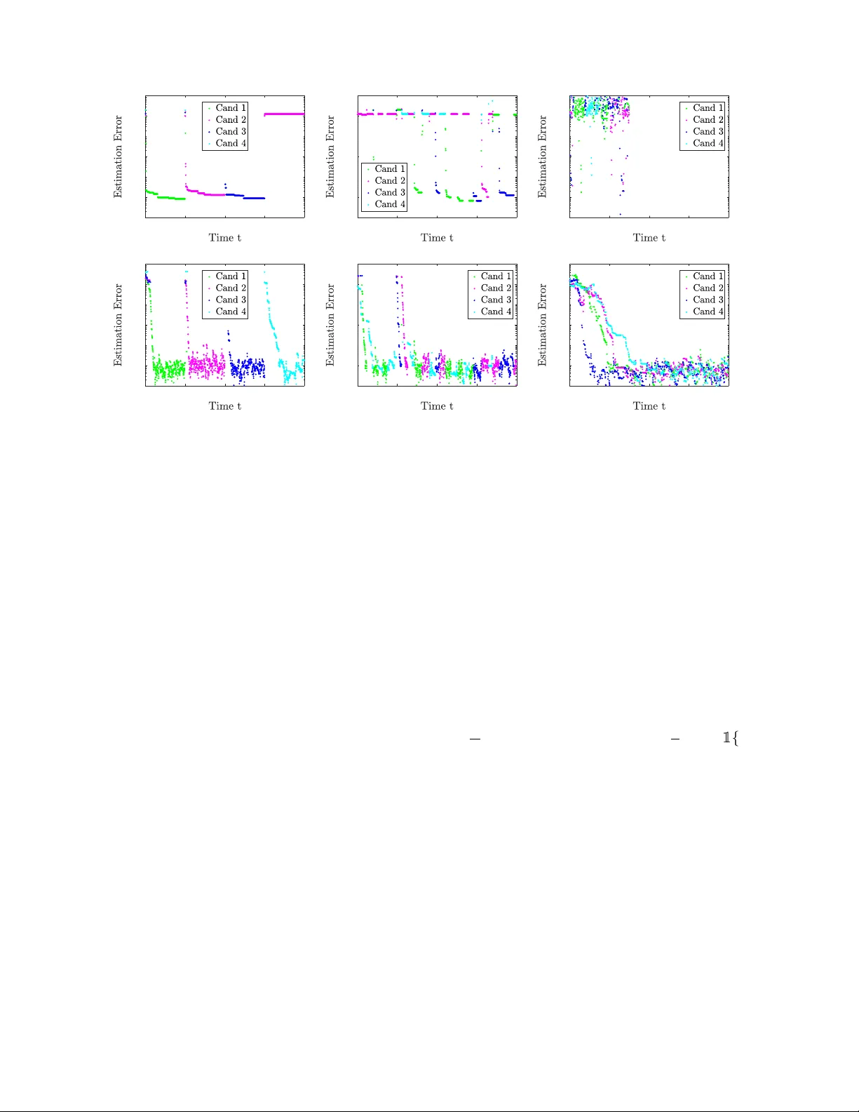
A Robust Algorithm for Online Switc hed System Iden tification ∗ Zhe Du , Necmiy e Ozay , and Laura Balzano Electrical and Computer Engineering, Univ ersity of Mic higan { zhe du,ne cmiye,gir asole } @umich.e du Abstract In this paper, w e consider the problem of online identification of Switc hed AutoRegressive eX- ogenous (SARX) systems, where the goal is to estimate the parameters of eac h subsystem and iden tify the switc hing sequence as data are obtained in a streaming fashion. Previous works in this area are sensitive to initialization and lack theoretical guaran tees. W e ov ercome these drawbac ks with our t w o-step algorithm: (i) ev ery time w e receive new data, w e first assign this data to one candidate subsystem based on a nov el robust criterion that incorp orates b oth the residual error and an upper b ound of subsystem estimation error, and (ii) we use a randomized algorithm to up date the parameter estimate of c hosen candidate. W e pro vide a theoretical guaran tee on the lo cal con ver- gence of our algorithm. Though our theory only guarantees conv ergence with a go od initialization, sim ulation results sho w that ev en with random initialization, our algorithm still has excellent p er- formance. Finally , we sho w, through simulations, that our algorithm outp erforms existing metho ds and exhibits robust p erformance. Keywor ds: System iden tification, Online iden tification algorithm, Conv ergence analysis 1 In tro duction A SARX system is a sp ecial type of hybrid system comp osed of multiple subsystems/mo des each with differen t parameters. At each time step only one subsystem is dominating and the dominan t subsystem ma y switch ov er time. Given system inputs and outputs at each time step, our goal is to identify the switc hing sequence (discrete states) as well as to estimate the parameters of the subsystems ev ery time w e receive new data. This is a problem in volving b oth clustering and estimation. In additional to applications in adaptiv e control, SARX system iden tification has b een applied to video and texture segmentation [13, 10, 11]. Due to the autoregressive nature of SARX mo del, it can also b e applied to earthquake record analysis [7], brain electrical activit y mapping [9], meteorological ob jects identification [3], and financial time series analysis [4]. 1.1 Prior W ork There ha ve been many studies on the switched system identification problem in the offline/batch setting. A t yp e of algebraic metho d was prop osed in [14], which uses V eronese embedding to decouple the task of estimating the system parameters and switc hing sequence, and an exact solution is pro vided when the pro cess and data are noise-free. F urthermore, the case when system orders are not necessarily ∗ This work is supp orted by DARP A grant N66001-14-1-4045, DARP A grant 16-43-D3M-FP-037 and NSF Grant ECCS-1508943. 1 equal or kno wn is discussed in [8]. F or systems with noise and measuremen ts corrupted by outliers, [10] extends the algebraic metho d by conv erting it to a rank minimization problem that is relaxed to a semi-definite program. Metho ds utilizing sparsity are prop osed in [1, 11]. As opp osed to the offline/batch setting, where we hav e access to all the data at once, there are man y problems in which the data app ears in a streaming (online) fashion. That is, at eac h time step, w e receive data with which w e need to iden tify current dominant subsystem as well as give the latest estimate of the system parameters. Note that naively emplo ying an offline algorithm b y using all the data in the past at each step w ould b e computationally in tractable. The ma jorit y of online algorithms use a t w o-step approach that alternates b et ween determining the switc hing sequence and up dating the parameter estimates. The work in [13] is one of the first to study online identification of switc hed systems using an extension of the offline algebraic metho d [14]. In the algorithms prop osed in [2], [5], candidate estimates are built for each of the subsystems first. Then, ev ery time a new data p oin t arriv es, the discrete state is determined b y assigning the data to one of the candidates according to some criterion, and then the estimate of chosen candidate is updated with the new data. The algorithm in [2] first identifies the discrete states based on prior or p osterior residual error, and then up dates the estimate using recursive least squares. The algorithm in [5] identifies the discrete states by minimizing prior residual error similarly and then up date the estimates with a mo dified Outer Bounding Ellipsoid (OBE) algorithm. 1.2 Con tributions and Outline W e observe that in tw o-step algorithms, c ho osing a candidate based on minim um residual error can b e sensitiv e to candidate initializations, since when a new subsystem dominates, it might “tak e-ov er” a partially con v ergent candidate estimate if there is no candidate y et closer to its true parameters. The main contribution of our pap er is a more robust tw o-step algorithm that can effectively ov er- come this issue. W e initialize candidate estimates for eac h of the subsystems. Ev ery time w e receiv e new data, we determine the discrete state b y assigning this data to one of candidates based on a robust criterion that incorp orates b oth residual error and an upp er b ound of estimation error. After w e assign the data to a candidate, w e up date the selected candidate using a v ariant of the randomized Kaczmarz algorithm prop osed in [12] or normalized least mean squares (NLMS) [6]. W e pro vide partial and lo cal conv ergence results for our algorithm. In our partial conv ergence analysis we assume that w e can alw ays make correct assignments, i.e. iden tify the discrete state correctly , thus the parameter estimation up dated for the candidates can b e treated as if we are using data from a single subsystem. In local conv ergence analysis, we assume all candidate estimates hav e “goo d enough” initializations, and show that with some probabilit y no misassignment will ever b e made and prov e the conv ergence of parameter estimates. Our n umerical sim ulations verify the con v ergence result and show obvious impro vemen ts of our algorithm ov er state of the art. The pap er is organized as follows: in Section 2, w e present the problem form ulation of online SARX system identification; Section 3 briefly discusses the drawbac ks of existing algorithms; Section 4 introduces our algorithm; Section 4 gives the theoretical analyses of our algorithm; some discussions and extensions are pro vided in Section 6; simul ation ev aluation are given in Section 7. 2 Problem F orm ulation 2.1 SARX System A SARX system is defined by the following expression: y t = X n a j =1 a j ( z t ) y t − j + X n c k =1 c k ( z t ) u t − k + n t (1) 2 where u t ∈ R and y t ∈ R are the input and output of the system, and n t ∈ R is an additive noise term. The discrete state z t ∈ { 1 , . . . , m } ≡ [ m ] indexes the dominant/activ e subsystem at time t , and { z t } t denotes the switching sequence. Co efficien ts { a j ( z t ) } n a j =1 and { c j ( z t ) } n c j =1 are the parameters of sub- system z t . Let φ y ,t = [ y t − 1 , . . . , y t − n a ] | , φ u,t = [ u t − 1 , . . . , u t − n c ] | , φ t = [ φ | y ,t , φ | u,t ] | , and furthermore, let w z t = [ a 1 ( z t ) , . . . , a n a ( z t ) , c 1 ( z t ) , . . . , c n c ( z t )] | . With this notation, the SARX system dynamics (1) can b e written in vector form: y t = w | z t φ t + n t . (2) Let n = n a + n c b e the system order, whic h can also b e view ed as the ambien t dimension of our problem. 2.2 Assumptions In this work, we mak e the following assumptions, where Assumption 1 and the noise upp er b ound in Assumption 2 are needed for the algorithm to w ork. (Case where noise is unbounded is discussed in Section 6.2.) Assumption 2 to Assumption 5 are mainly for analysis purp oses. Assumption 1. The mo del or ders n a , n c on RHS of (1) , and the numb er of subsystems, m , ar e known. Assumption 2. The noise n t is r andom with E [ n t ] = 0 and E [ n 2 t ] = σ 2 n . | n t | ≤ n max and n max is known. n t is indep endent of input u t . Assumption 3. F or al l t , k φ t k ≤ φ max . We also assume a lower b ound on the SNR: for al l t, k φ t k | n t | ≥ S min . Assumption 4. Ther e exists s max ≥ s min > 0 such that ∀ S ⊂ N + with c ar dinality N R (define d in Se ction 4), s 2 min I n  X t ∈ S φ t φ | t  s 2 max I n . (3) Assumption 5. If subsystem i gener ates data p air { φ t , y t } , i.e. y t = w | i φ t + n t , then ∀ j 6 = i , | w | j φ t − w | i φ t | ≥ ψ . Assumption 4 is similar to p ersisten t excitation conditions in the literature, and it pla ys a critical role in the conv ergence rate. Assumption 5 guarantees there is no am biguous data, since if data pair { φ t , y t } satisfies b oth y t = w | 1 φ t and y t = w | 2 φ t , then ev en with the true parameters w 1 and w 2 , w e cannot tell whic h system generates y t . 2.3 Goal The goal of online system identification is as follows. After w e collect the data pair { φ t , y t } at eac h time step, we w an t to identify discrete state z t and estimate parameters of the subsystem that generates y t . 3 Dra wbac ks of Existing Algorithms Existing algorithms e.g. [2], [5], commonly hav e a t wo-step structure after candidate estimate for eac h of the subsystem is initialized: (1) ev ery time new data is av ailable, it is assigned to the candidate with minimum prior/p osterior residual error; (2) the parameter estimate of the chosen candidate is up dated with this data. W e will sho w that using only residual error as the criterion to assign data can b e unreliable. Fig. 1 shows a to y example of what could go wrong with the ab ov e mentioned algorithms. There are 3 subsystems, and red circles illustrate their true parameter vectors in the ambien t space; the 3 Figure 1: Demonstration of potential drawbac k of existing algorithms. 3 candidate estimates are initialized at the three dark blue p oin ts in the left b o x. Assume from t = 1 to 10, subsystem 1 is dominant (left b o x), and from t = 11 to 20, subsystem 2 is dominant (right b o x). Considering the p ositions and true and estimated parameters, it’s likely that from t = 1 to 10 data generated by subsystem 1 will b e assigned to candidate 1 since it’s the closest candidate. When t = 10, candidate 1 is an impro ved estimate of system 1 parameters, giv en b y the light blue p oin t in the left b o x. At time t = 11, subsystem 2 b ecomes dominant. Considering the current p ositions of all candidates, candidate 1 is still closest to subsystem 2, so it’s likely that data generated b y subsystem 2 will also b e assigned to candidate 1, and w e could exp ect candidate 1 will start to drift from subsystem 1 parameter v alues tow ard subsystem 2, given b y the tra jectory in the righ t b ox. In this sense, all previous efforts used to let candidate 1 learn subsystem 1 will b e w asted. In our algorithm, the basic idea to solv e this drawbac k is to take the accuracy of the candidate estimates into account and b e more cautious when assigning data to candidates with higher accuracy . The details will b e discussed in Section 4.1. 4 Our Algorithm In this pap er we prop ose Algorithm 1 for online iden tification of SARX mo dels. This is also a tw o-step algorithm, but with an impro ved data assignmen t to consider not only the residual but also system estimation accuracy . This section gives an ov erview of the algorithm steps. Lines 1 to 4 sho w initialization. b w i, 0 is the initial estimate for candidate i , and c i is num b er of assignmen ts to candidate i . Φ R i,t ∈ R n x N R , y R i,t ∈ R N R , Φ C i,t ∈ R n x N C , c W C i,t ∈ R n x N C , h C i,t ∈ R N C ,  u i,t are the corresp onding windo w v ariables for candidate i at time t , whic h will b e explained in details later in this section. N R and N C are the n um b er of columns of Φ R i,t and Φ C i,t resp ectiv ely , whic h are also the windo w lengths for the randomized Kaczmarz algorithm and error upp er b ound estimation resp ectiv ely . A t each time step, via Lines 6 to 13, we assign the data to one of the candidates using a new criterion to determine the discrete state. Then, w e up date the c hosen candidate estimate using an idea similar to the randomized Kaczmarz algorithm in [12] in Lines 14 to Line 24. 4.1 Making Assignment/Iden tifying the Discrete State With data pair { φ t , y t } , w e compute the normalized residual error r i for eac h candidate in Line 8, where b w i,t − 1 is the estimate of candidate i at time t − 1. W e then compute the p otential new estimate e w i,t for eac h candidate if w e were to use { φ t , y t } to up date b w i,t − 1 . The assignmen t criterion is given in Line 11. The criterion has tw o comp onen ts: the first term is the normalized residual error r i and the second term measures whether e w i,t has a larger estimation error than b w i,t − 1 . The v ariables α , β and ν are tuning parameters. V ariable  u i,t − 1 is an estimate of upp er b ound on the magnitude of candidate i ’s estimation error  i,t − 1 ≡ w − b w i,t − 1 with resp ect to 4 Algorithm 1: Our Main Algorithm 1 Initialize N R , N C ( N R ≥ n, N C ≥ N 2 R ) , α, β , ν 2 for i = 1 , . . . , m do 3 b w i, 0 = 0 n × 1 , c i = 0 , Φ R i,t = 0 n × N R , y R i,t = 0 N R × 1 , 4 Φ C i,t = 0 n × N C , c W C i,t = 0 n × N C , h C i,t = 0 N C × 1 ,  u i, 0 = ∞ 5 for t = 1 , 2 , . . . do 6 Receiv e { φ t , y t } . 7 Compute normzlized residual errors and p oten tial new estimates for all candidates: 8 r i = | y t − b w | i,t − 1 φ t | · k φ t k − 1 ∀ i ∈ [ m ] 9 e w i,t = b w i,t − 1 −k φ t k − 2 φ t ( b w | i,t − 1 φ t − y t ) ∀ i ∈ [ m ] 10 Cho ose a candidate to assign data: 11 b z t = arg min i r i · max  1 , α k e w i,t − b w i,t − 1 k 2(  u i,t − 1 + ν )  β 12 Up date counter and window v araibles: 13 c b z t = c b z t + 1 14 Φ R ˆ z t ,t =[ Φ R ˆ z t ,t − 1 [: , 2:end] , φ t ] , y R ˆ z t ,t =[ y R ˆ z t ,t − 1 [2:end]; y t ] 15 Up date estimate of chosen candidate: 16 if c b z t < N R then 17 φ ∗ t = φ t , y ∗ t = y t , η ∗ t = k φ t k − 2 18 else 19 Sample l t ∈ [ N R ] w.p. k Φ R b z t ,t [: , l t ] k 2 / k Φ R b z t ,t k 2 F 20 φ ∗ t = Φ R b z t ,t [: , l t ] , y ∗ t = y R b z t ,t [ l t ] , η ∗ t = k φ ∗ t k − 2 21 b w b z t ,t = b w b z t ,t − 1 − η ∗ t φ ∗ t ( b w | b z t ,t − 1 φ ∗ t − y ∗ t ) 22 Up date error upp er b ound and windo w v ariables: 23 Φ C b z t ,t , c W C b z t ,t , h C b z t ,t ,  u b z t ,t = Up dateUpperBound 24 ∀ i 6 = b z t , { b w i,t , Φ R i,t , y R i,t , Φ C i,t , c W C i,t , h C i,t ,  u i,t } = { b w i,τ , Φ R i,τ , y R i,τ , Φ C i,τ , c W C i,τ , h C i,τ ,  u i,τ } τ = t − 1 some true system parameter w . The main difference b et ween our algorithm and previous tw o-step algorithms men tioned in Section 3 is the incorp oration of the second term, whic h makes assignment more robust. Figure 2: Idea of our algorithm The idea b ehind the criterion is straightforw ard: letting α =1 , β =1 , ν =0, and replacing  u i,t − 1 with k  i,t − 1 k , the second part of the criterion b ecomes max  1 , k e w i,t − b w i,t − 1 k 2 k  i,t − 1 k  . The n umerator k e w i,t − b w i,t − 1 k 5 is the magnitude of v ariation if w e up date the estimate b w i,t − 1 of candidate i with { φ t , y t } . W e could see that if the estimation error of e w i,t do esn’t increase compared with the error of b w i,t − 1 , then we m ust hav e k e w i,t − b w i,t − 1 k ≤ 2 k  i,t − 1 k . And if k e w i,t − b w i,t − 1 k > 2 k  i,t − 1 k , then the estimation error m ust get larger. Therefore, max  1 , k e w i,t − b w i,t − 1 k 2 k  i,t − 1 k  w orks against candidates whose error w ould increase if we up date using { φ t , y t } . The max op erator sho ws that as long as k e w i,t − b w i,t − 1 k ≤ 2 k  i,t − 1 k , w e don’t p enalize an y further. Since we don’t know the true estimation error k  i,t − 1 k , we replace it with its estimated upp er b ound  u i,t − 1 (w e will show under some conditions, this is a v alid upp er b ound in Theorem 9) computed in Algorithm 2. This idea is illustrated with Fig. 2. Consider the same experimental setup as the to y example in Section 3. At time t = 11, candidate 1 will b e within the ball region (denoted with the red dotted circle) estimated by upp er b ound  u . Once the p oten tial up date magnitude of candidate 1 exceeds the diameter 2  u of this region, which implies its estimation accuracy will b ecome worse if we up date candidate 1 with this data, so candidate 1 should b e p enalized when making the assignment. W e note that k e w i,t − b w i,t − 1 k≤ 2 k  i,t − 1 k is only a necessary but not sufficient condition to ensure non-increasing estimation error. Even though we are relying on a necessary condition, our algorithm empirically ac hieves significan tly improv ed p erformance o v er previous algorithms. 4.2 Candidate Estimate Up dates After the assignment is made, from Line 14 to Line 21 w e up date the estimate of the candidate b z t to which the data has been assigned. Our up dating approach is based on the randomized Kaczmarz metho d with a sliding window of data. W e define window v ariables Φ R i,t , y R i,t to store previous N R data { φ , y } assigned to candidate i . If w e hav e collected N R data, i.e. c b z t ≥ N R , we up date the estimate with randomly pic ked historical data { φ ∗ t , y ∗ t } ; otherwise we simply up date using current data { φ ∗ t , y ∗ t } = { φ t , y t } . The idea b ehind the up date rule is that we pro ject the current estimate b w b z t ,t − 1 on to the solution space of { φ ∗ t , y ∗ t } suc h that y ∗ t = b w | b z t ,t φ ∗ t . 4.3 Computation of Error Upp er Bound W e up date the error upp er b ound estimate  u b z t ,t and related windo w v ariables Φ C b z t ,t , c W C b z t ,t , h C b z t ,t of the c hosen candidate in Line 23. The details of this up date are given in Algorithm 2. If the windo w is not full, i.e. c b z t 0 , we have P   t \ τ = N R  k  i,τ k 2 ≤  0 2    ≥ 1 − E  k  i,N R − 1 k 2   0 2 (15) Lemma 15. Assume Assumption 13 holds. With Setup(A), for some  0 > 0 , assume k  i, 0 k ≤  0 such that r N R   2 0 + N R S 2 min  ≤  0 , then for ∀ t we have P t \ τ =1  k  i,τ k 2 ≤  0 2  ! ≥ 1 − 2 s N R  0 2   2 0 + N R S 2 min  (16) Lemma 16. L et  0 = 1 2 φ max  ψ − n max ν S min − 3 n max  , α = 2 , and β = 1 . Assume at time t , c andidates ar e one-to-one  0 -close to subsystems. WLOG, we c ould assume ∀ i, k  i,t − 1 k ≡ k w i − b w i,t − 1 k ≤  0 . F urthermor e, we assume that al l assignments prior to time t ar e made c orr e ctly, i.e. ∀ s < t, b z s = z s . Then at time t , we wil l also assign data c orr e ctly, i.e. b z t = z t . Theorem 17 (Lo cal Con vergence) . Assume Assumption 13 holds. L et  0 = 1 2 φ max  ψ − n max ν S min − 3 n max  , α = 2 , and β = 1 . L et  i,t = w i − b w i,t denote the estimation err or of c andidate i at time t . WLOG, assume ∀ i, k  i, 0 k ≤  0 such that r N R   2 0 + N R S 2 min  ≤  0 . Then ∀ i, t such that r ( i, t ) ≥ N R , with pr ob a- bility at le ast 1 − 2 m r N R  0 2   2 0 + N R S 2 min  , we have the fol lowing r esults: (i). We c an c orr e ctly identify the switching se quenc e, i.e. ∀ t, b z t = z t . In another way, ∀ i, t , { φ t , y t } fr om subsystem i wil l b e assigne d to c andidate i . (ii). R esults for (12) , (13) and (14) wil l hold. Corollary 18 (Local Conv ergence Without Noise) . L et n t = 0 , i.e. ther e is no noise. L et  0 = ψ 2 φ max , α =2 , and β =1 . L et  i,t = w i − b w i,t denote the estimation err or of c andidate i at time t , and assume ∀ i, k  i, 0 k ≤  0 such that p N R  2 0 ≤  0 . Then ∀ i, t such that r ( i, t ) ≥ N R , with pr ob ability at le ast 1 − 2 m q N R  0 2  2 0 , we have the fol lowing r esults: (i). We c an c orr e ctly identify the switching se quenc e, i.e. ∀ t, b z t = z t . In another way, ∀ t, ∀ i , 9 { φ t , y t } fr om subsystem i wil l b e assigne d to c andidate i . (ii). we have the fol lowing c onver genc e r esults: ∀ i, t such that r ( i, t ) ≥ N R E  k  i,t k 2  ≤  1 − κ − 2 max  r ( i,t ) − N R +1 k  i, 0 k 2 (17) If as t →∞ , we have r ( i, t ) →∞ , i.e. subsystem i c an dominate infinitely often, then as t →∞ , we have E  k  i,t k 2  =0 . 6 Discussions and Extensions 6.1 P oles, Condition Num b er, and Conv ergence Rate Systems with p oles close to the unit circle are not preferable as they are close to b e unstable. In algorithm conv ergence analysis, Hessian matrix or ob jectiv e function with large condition num b er is usually not preferable as the con vergence rate tends to get small. In this section, we will show how these t wo facts meet consistently in our algorithm. That is, as the system p oles getting closer to the unit circle, the condition num b er of Hessian matrix will get larger, and the conv ergence rate of upp er b ound in (12) will get smaller. T o study the conv ergence rate, it suffices to study a single subsystem without any switching. W e drop the subsystem subscript, and let  t = w − b w t denote the estimation error. Since the goal of this section is to provide insight in to the relations b et ween p oles, condition num b er, and con vergence rate, so sev eral steps in volv e approximation. And when study how p oles affect the condition num b er, we only consider a toy system with order 3, since it is c hallenging to find nice analytical expressions for systems with higher order. First w e consider ho w condition num b er influences conv ergence the rate of upp er b ound in (12). 6.1.1 Condition Num b er vs. Conv ergence Rate The expression for single ARX system is given b y y t = P n a j =1 a j y t − j + P n c k =1 c k u t − k + n t = w | φ t + n t follo wing our notations in Section 2. In Assumption 4, we hav e s 2 min I n  P t ∈ S φ t φ | t  s 2 max I n . W e will see this equation is related to the correlation matrix R ≡ E [ φ t φ | t ], if it exists. In [6], we could kno w for the ARX system given ab o ve, if (i) p oles of system are within the unit circle, and (ii) noise is white Gaussian and input is wide-sense stationary , then there exists R such that lim t →∞ E [ φ t φ | t ] = R . When N R is large, according to law of large num b ers, equation (3) and the result ab o ve, we hav e lim min( S ) →∞ P t ∈ S φ t φ | t ≈ N R R . W e let λ max , λ min denote the maximum and minimum eigen v alue of R . Now dropping the “lim” and replace “ ≈ ” with “=”, w e could get N R λ min I n  P t ∈ S φ t φ | t  N R λ max I n . So N R λ min and N R λ max are equiv alent to s 2 min and s 2 max defined in Assumption 4. Then according to Lemma 6, we could hav e κ max = p ( n − 1) λ max /λ min +1 and ξ min = p ( n − 1) λ min /λ max +1. So, for the asymptotic conv ergence upp er b ounds in (10), (12), and (17) which all in volv e κ max , when the condition n umber of R , λ max /λ min , increases, κ max will increase, and the conv ergence rate in upp er b ounds will decrease. 6.1.2 P oles vs. Condition Num b er W e consider a to y example of system with order 3: y t = a 1 y t − 1 + a 2 y t − 2 + c 1 u t − 1 + n t = w | φ t + n t where w ≡ [ a 1 , a 2 , c 1 ] and φ t ≡ [ y t − 1 , y t − 2 , u t − 1 ]. W e assume all poles are within the unit circle, 10 u t ∼ N (0 , σ 2 u ), n t ∼ N (0 , σ 2 n ), u t ⊥ n t , u t ⊥ u s , n t ⊥ n s , ∀ t, s , and σ u  σ n . F ollo wing [6], we hav e R = E  φ t φ | t  =   r (0) r (1) 0 r (1) r (0) 0 0 0 σ 2 u   (18) where r (0) , r (1) can b e computed by solving   r (0) r (1) r (2)   =   1 − a 1 − a 2 − a 1 1 − a 2 0 − a 2 − a 1 1   − 1   σ 2 n + c 1 σ 2 u 0 0   (19) So, w e ha ve R = E  φ t φ | t  =   ( a 2 − 1) c ( − a 1 ) c 0 ( − a 1 ) c ( a 2 − 1) c 0 0 0 σ 2 u   (20) where c = σ 2 n + c 1 σ 2 u ( a 2 +1)( a 1 + a 2 − 1)( a 1 − a 2 +1) . W e will drop σ 2 n in the follo wing computation as σ u  σ n . The eigen v alues of R are given by λ 1 = − c 1 σ 2 u ( a 2 + 1)( a 1 + a 2 − 1) (21) λ 2 = c 1 σ 2 u ( a 2 + 1)( a 1 − a 2 + 1) (22) λ 3 = σ 2 u (23) Note that the p oles p 1 , p 2 satisfy p 1 + p 2 = a 1 and p 1 p 2 = − a 2 , so w e ha ve λ 1 = c 1 σ 2 u (1 − p 1 p 2 )(1 − p 1 )(1 − p 2 ) (24) λ 2 = c 1 σ 2 u (1 − p 1 p 2 )(1 + p 1 )(1 + p 2 ) (25) λ 3 = σ 2 u (26) Let c 1 ≥ 1, since p 1 , p 2 < 1, we can see the condition n um b er of R will hav e the following low er b ound λ max λ min ≥ λ 1 λ 3 = 1 (1 − p 1 p 2 )(1 − p 1 )(1 − p 2 ) (27) It’s easy to see as p oles get closer to the unit circle, this low er b ound will get larger and the condition n umber is lik ely to increase as w ell. 6.1.3 P oles vs. Conv ergence Rate Finally , by com bining the t w o results w e just show ed, we could see as the system p oles getting closer to unit circle, the con v ergence rate of upp er b ound in (12) will decrease. There are t w o commen ts regarding this conclusion. (i) Even though this result only inv olv es the rate of upp er b ound , empirical results show the true con vergen t rate follo w accordingly; (ii) Our algorithm fa vors stable system whic h is a little coun terintuitiv e as unstable system tends to hav e higher SNR. 11 6.2 Un b ounded Noise and Mon te Carlo Metho d Note that w e compute the error upp er b ound  u b z t ,t in Line 15 of Algorithm 2 by finding the maximum k A n − b k from cub e vertices V defined by the noise magnitude upp er b ound n max . How ev er, if n max is unkno wn or the noise itself is un b ounded, e.g. Gaussian, Algorithm 2 is not applicable to ev aluate  u b z t ,t . In this case, if w e could ha ve samples of noise instead, an alternative approac h is to use Mon te Carlo metho d to ev aluate  u b z t ,t . Sp ecifically , if w e hav e N t samples of noise v ector n t (defined in the pro of for Theorem 9) given by { n ( i ) t } N t i =1 , we could let  u b z t ,t = max k A n ( i ) t − b k . Due to the Monte Carlo nature, this is not necessarily a v alid upp er b ound. In another wa y , the result in Theorem 9 do esn’t hold, i.e.  u b z t ,t < k  b z t ,t k . Practically , algorithm still has satisfactory p erformance when using this Mon te Carlo metho d, but theoretically , this ma y not guarantee lo cal con vergence since lo cal conv ergence result Theorem 17 implicitly Theorem 9, i.e.  u b z t ,t ≥ k  b z t ,t k , to hold for every time step. If w e prefer the theoretical guarantees to practical implemen tation, by subtly designing the n umber of Monte Carlo samples N t at time t , there could b e some probabilit y guarantee to ensure  u b z t ,t is a v alid upp er b ound at ev ery time step. F or ease of illustration, we assume there is only one subsystem, then w e could drop the subsystem index subscript, and replace  u b z t ,t with  u t ,  b z t ,t with  t . And we assume the Monte Carlo metho d starts at time 1. Then w e hav e the following theorem: Theorem 19. If we use Monte Carlo metho d ab ove to c ompute  u t , for some ζ 1 , ζ 2 ∈ (0 , 1) , let N t ≥ ζ 2 t 2 ζ 2 t 1 , then P P ∞ \ t =1 {k  t k≤  u t } ! ≥ 1 − ζ 1 1 − ζ 1 ! ≥ 1 − exp( − ζ 2 ) 1 − exp( − ζ 2 ) (28) In another wor d, the pr ob ability that every  u t is a valid upp er b ound is lar ge with a lar ge pr ob ability. The pro of for this theorem is again in the app endices. W e can immediately see from Theorem 19 that in order to make the probabilities large, the n um b er of Monte Carlo samples need to increase exp onen tially with resp ect to time, whic h mak es implemen tation intractable when time is long. 6.3 Extension to MIMO Case So far we hav e b een a considering SISO system in (1), where all the y t and u t are scalars. Ho w ev er, our algorithm can b e applied to MIMO systems with some transformation of the system equation, and w e will pro vide a p otential direction in this section. Let y t ∈ R n y , u t ∈ R n u , then the MIMO SARX system is given by y t = n a X j =1 A j ( z t ) y t − j + n c X k =1 C k ( z t ) u t − k + n t (29) where { A j ( z t ) } n a j =1 , { C j ( z t ) } n c j =1 are the parameters of subsystem z t . Let W z t = [ A 1 ( z t ) , . . . , A n a ( z t ) , C 1 ( z t ) , . . . C n c ( z t )] | , φ t = [ y | t − 1 , . . . , y | t − n a , u | t − 1 , . . . , u | t − n c ] | . Let w z t ,i denote the i th column of W z t , and let y t,i , n t,i denote the i th element in y t and n t . Then the MIMO system can b e broken into a set of equations: ∀ i ∈ [ n y ], y t,i = w | z t ,i φ t + n t,i (30) whic h has the same form as (1). So we could mo dify our algorithm to estimate each w z t ,i in a parallel w ay , then combine them to estimate W z t . 12 6.4 Multiple N C ’s and F orgetting F actor 6.4.1 Multiple N C ’s Note that in Algorithm 2, w e hav e windo w v ariables Φ C i,t ∈ R n x N C , c W C i,t ∈ R n x N C , h C i,t ∈ R N C for some windo w length N C to compute the error upp er b ound  u b z t ,t . Theorem 9 says when all data stored in the window are from the same subsystem, then  u b z t ,t will b e a v alid error upp er b ound with resp ect this subsystem. Ho w ever, if there enters some outlier data (data generated by subsystem that is differen t from the subsystem that generates the ma jorit y of data in the window v ariables),  u b z t ,t computed using windo w v ariables might be an inv alid upp er bound. If the window length is too large, since the windo w is sliding, the effect of outlier will stay a longer time, but the correction effect of the ma jority of the inlier data migh t reduce the effect of outlier. On the contrary , if the window length is too small, the effect of outlier will quickly v anish, but the correction effect from the inlier data will reduce as well and w e ma y hav e even worse  u b z t ,t during the sta y of outlier. Practically , we could use multiple N C ’s and corresp onding window v ariables. Each set of windo w v ariables compute  u b z t ,t separately , and w e pick the maximum of them as the final decision. In this w ay , the disadv antages of large and small windo w lengths migh t cancel out eac h other thus making  u b z t ,t more robust to misassignmen t. 6.4.2 F orgetting F actor One interesting fact ab out our algorithm is, in Line 19 of Algorithm 1, instead of using the latest data, we pic k randomly from previous data to up date the estimates. This idea is initially proposed in [12]. The reason we incorp orate this randomization in to the algorithm is to acquire the asymptotic con vergence result via Assumption 4, Lemma 6, Lemma 7, and Lemma 8. If no randomization scheme is utilized, the algorithm on a single subsystem is equiv alent to the Kaczmarz algorithm or the normalized least mean squares (NLMS) algorithm in [6]. This t yp e of algorithm, how ever, do es not hav e satisfactory c on vergence results y et. One linear conv ergence result pro vided in [6] is v alid only when the step size in estimate up date is v ery small, which makes it little practical use. The difficulty to derive nice conv ergence results is that nearb y data φ t could b e highly correlated, whic h can be seen from the definition, and updating the estimate with data in c hronological order aggrav ates the situation. The randomized scheme picks data for up date randomly and indep enden tly , whic h brings indep endence into the algorithm and makes analysis tractable. Empirically , if we don’t incorp orate the random selection in Line 19, and alw ays use latest data as Line 17, the p erformance can sometimes b e slightly b etter. This is p oten tially b ecause when sampling previous data vectors, it’s lik ely that we sample one data m ultiple times p ossibly due to its large norm, and, generally sp eaking, previously used data ma y not pro vide as muc h information as some new data. One potential wa y to balance betw een establishing theoretical results and exploiting new data is to incorp orate a forgetting factor γ . Sp ecifically , in Line 19, we sample data according to the follo wing distribution P ( l t = i ) ( γ k Φ R b z t ,t [: , i ] k 2 1 F if i = N R (1 − γ ) k Φ R b z t ,t [: , i ] k 2 1 F if if i < N R (31) where γ > 0 . 5, and F = γ k Φ R b z t ,t [: , N R ] k 2 + (1 − γ ) P N R − 1 i =1 k Φ R b z t ,t [: , i ] k 2 is the normalization factor. With this distribution, we can see the probability of choosing the latest data ( l t = N R ) is larger compared with the distribution in Algorithm 1. As γ gets closer to 1, we are more lik ely to sample the latest data. As for the con vergence result, it suffices to only consider how the building block lemmas will c hange with this new distribution, and the main theorems will follow these lemmas. In the building blo c k lemmas, only the exp ectations in Lemma 7 (iii), and Lemma 8 in volv e the data sampling process. With the new sampling distribution, it’s not difficult to see (7) and (8) will b ecome 13 ˜ γ − 1 N R F 2 max σ 2 n ≤ E " n 2 r t ( l t ) k φ r t ( l t ) k 2 # ≤ ˜ γ N R F 2 min σ 2 n (32) ˜ γ − 1 κ − 2 max E [ k z k 2 ] ≤ E   φ | r t ( l t ) z k φ r t ( l t ) k ! 2   ≤ ˜ γ ξ − 2 min E [ k z k 2 ] (33) where ˜ γ = γ 1 − γ > 1. The rest of the lemmas, theorems, corollaries follo w from these new results. 7 Numerical Results In this section, w e use simulation examples to ev aluate the theoretical results as w ell as the performance of our algorithm. 7.1 Ev aluation of Asymptotic Con vergence Bounds Since it is not con v enient to visualize the con vergence b ounds for SARX system with multiple sub- systems, and (10) and (11) give tighter p erformance than (13) and (14), w e will ev aluate the low er and upp er asymptotic conv ergence b ounds in (10) and (11) on single ARX system by comparing the b ounds with the actual conv ergence b eha vior. Consider a sp ecific system y t = 0 . 7 y t − 1 − 0 . 12 y t − 2 + u t − 1 + n t (34) where n t ∼ N (0 , σ 2 n ), σ n = 10 − 4 , u t ∼ N (0 , 1). According to Section 6.1, the correlation matrix is giv en by R =   1 . 67 1 . 04 0 1 . 04 1 . 67 0 0 0 1   (35) , and its minim um and maxim um eigen v alues are λ min = 0 . 63 and λ max = 2 . 71. Since it’s difficult to hav e exact knowledge of κ max and ξ min , we will use the approximate v alues defined in Section 6.1, i.e. κ max = p ( n − 1) λ max /λ min +1 and ξ min = p ( n − 1) λ min /λ max +1. And similarly , we could hav e F max = √ nN R λ max and F min = √ nN R λ min . W e set N R = 10 and simulation time horizon T = 1000. T o ev aluate the exp ectation E  k  i,t k 2  in (10) and (11), we run the algorithm 50 times with different realizations of input u t , noise n t , and random data s election in Line 19 of Algorithm 1, and take the a v erage of estimation errors as the exp ectation. The simulation results are given in Fig. 3. W e can see the estimation error E  k  i,t k 2  can b e successfully b ounded by the upp er and low er b ound in (10) and (11). 7.2 Robust Behavior of our Algorithm 7.2.1 Single Realization Exp eriment First w e ev aluate our algorithm and compare it with the OBE algorithm in [5] using SARX system giv en b elow • Subsystem 1: y t = 0 . 2 y t − 1 + 0 . 24 y t − 2 + 2 u t − 1 + n t • Subsystem 2: y t = 0 . 7 y t − 1 − 0 . 12 y t − 2 + 1 u t − 1 + n t 14 0 100 200 300 400 500 10 -5 10 0 Figure 3: Ev aluation of conv ergence b ounds • Subsystem 3: y t = − 1 . 4 y t − 1 − 0 . 53 y t − 2 + 1 u t − 1 + n t • Subsystem 4: y t = 1 . 7 y t − 1 − 0 . 72 y t − 2 + 0 . 5 u t − 1 + n t where u t ∼N (0 , 1). n t follo ws N (0 , σ 2 n ) truncated to region [ − 3 σ n , 3 σ n ] where σ n =10 − 4 , so noise is b ounded with n max =3 σ n . T o fully ev aluate the p erformance, we consider 3 differen t switc hing patterns of subsystems: (i) Slow Switching (SS): subsystem 1 dominates from 1 to 500, subsystem 2 dominates from 501 to 1000, subsystem 3 dominates from 1001 to 1500, and subsystem 4 dominates from 1501 to 2000. (ii) Minimum Dwel l Time (MD): each subsystem dominates 30 time steps, and then the time it takes to switch to a new subsystem is a random v ariable following the geometric distribution with parameter 1 / 16. When the subsystem switches, all subsystems are equally lik ely to be switched to, and after the switching, this pro cess restarts again. (iii) F ast Switching (FS): at ev ery time step, ev ery subsystem dominates with equal probabilities. In our algorithm, we set N R =3 , N C =20 , α =4 , β =3 , ν =10 − 4 , and simulation time horizon T = 2000. The candidates are initialized with standard m ultiv ariate Gaussian distribution. After the algorithms completes all T time steps, we first relab el the candidates with a bijectiv e mapping h ( · ) : [ m ] → [ m ] suc h that P i ∈ [ m ] k w i − b w h ( i ) ,T k is minimized. In the fol lowing, the c andidates ar e r eferring to the r elab ele d c andidates. W e compute all the estimation errors, i.e.  i,t = w i − b w i,t , ∀ i, t , which measure the distance b et ween candidate i and subsystem i during the algorithm. Fig. 4 depicts the simulation results. The dots in the plots represent each k  b z t ,t k , ∀ t , which means there is only one dot plotted for one time step. Different colors corresp ond to different candidates and corresp onding true subsystems. F or example, if there exists a blue dot at time t = 1400, this means w e assign data generated at time t = 1400 to candidate 3, and current error b etw een candidate 3 and subsystem 3 is giv en b y the y-axis v alue of the dot. F rom the plots, we see that our algorithm conv erges more quickly than the OBE algorithm. Since none of the colors hav e a sharp increase in error, w e could claim the phenomenon describ ed in Section 3 is effectively av oided in these realizations. F or the OBE algorithm, the p erformance is ob viously w orse: in the FS case, none of the candidates ev en conv erge, and the algorithm even stops halfwa y due to numerical instabilit y . In the plots for SS-OBE, we can see the undesired phenomenon describ ed in Section 3: candidate 2 has con verged to the vicinit y of subsystem 2 from t = 501 to t = 1000, but after time t ≥ 1500, the error go es large again. This is b ecause w e are assigning data generated b y subsystem 4 to candidate 2, making candidate 2 mo v e tow ards subsystem 4. F rom these plots, we see 15 0 500 1000 1500 2000 10 -4 10 -2 10 0 (a) 0 500 1000 1500 2000 10 -4 10 -2 10 0 (b) 0 500 1000 1500 2000 10 -4 10 -2 10 0 (c) 0 500 1000 1500 2000 10 -4 10 -2 10 0 (d) 0 500 1000 1500 2000 10 -4 10 -2 10 0 (e) 0 500 1000 1500 2000 10 -4 10 -2 10 0 (f ) Figure 4: Estimation errors of OBE algorithm and our algorithm: (a) SS-OBE; (b) MD-OBE; (c) FS-OBE; (d) SS-Ours; (e) MD-OBE; (f ) FS-Ours that our algorithm outp erforms OBE algorithm for all switc hing patterns. 7.2.2 Multiple Realizations Exp eriment Since a single realization cannot comprehensively ev aluates the p erformance, we further compare our algorithm with the OBE algorithm using multiple realizations. Sp ecifically , we consider 9 exp er- imen t setups, given b y all the combinations of switching patterns { SS, MD, FS } and noise lev el σ n ∈ { 10 − 1 , 10 − 2 , 10 − 3 } , and for each of the exp erimen t setup, we run M =100 realizations. Each subsystem parameters are generated randomly in each realization: w e first sample 2 real p oles on [ − 1 , 1] uniformly , and then compute the parameters from the sampled poles. The rest of the setups, e.g. n umber and orders of subsystems, algorithm parameters, etc., follo w the previous single realization exp erimen t. F or realization i , we define the t wo metrics: FE( i ) = 1 m P m j =1 k  j,T k and CER( i ) = 1 T P T t =1 1 { z t 6 = b z t } . FE measures the final estimation error and CER is the classification error rate. T able 1 lists the a verage FE and CER v alues ov er all 100 realizations. W e could see, our algorithm exhibits b etter p erformance in each setup. 8 Conclusions In this pap er, we in tro duced a robust algorithm to solv e online switched system iden tification problem. Our algorithm follows the conv entional tw o-step framework, but the modified assignment criterion leads to a more robust assignment pro cess. After w e assign the data to some candidate, w e update the candidate estimate based on the idea of randomized Kaczmarz algorithm. W e sho wed partial and lo cal conv ergence results. The partial conv ergence result is: assuming there is no misassignmen t, then the estimation error conv erges geometrically to some quan tit y related to noise v ariance in the exp ectation square sense. The lo cal conv ergence result is: assuming all candidates ha ve go o d enough initialization, with some probability , it can b e guaran teed that no misassignment will b e made, and 16 T able 1: Results for Multiple Realizations Exp erimen t Ours OBE Ours OBE FE FE CER CER SS, 10 − 1 8 . 4 x 10 − 1 8 . 7 x 10 − 1 56 . 3% 59 . 1% SS, 10 − 2 2 . 8 x 10 − 2 8 . 2 x 10 − 1 22 . 1% 55 . 5% SS, 10 − 3 9 . 0 x 10 − 2 8 . 2 x 10 − 1 8 . 35% 56 . 4% MD, 10 − 1 4 . 3 x 10 − 1 5 . 2 x 10 − 1 47 . 5% 50 . 3% MD, 10 − 2 4 . 0 x 10 − 2 2 . 8 x 10 − 1 11 . 3% 31 . 3% MD, 10 − 3 9 . 4 x 10 − 3 2 . 4 x 10 − 1 4 . 91% 28 . 8% FS, 10 − 1 2 . 6 x 10 − 1 6 . 8 x 10 − 1 39 . 3% 53 . 9% FS, 10 − 2 6 . 0 x 10 − 2 1 . 5 x 10 − 1 11 . 7% 22 . 1% FS, 10 − 3 5 . 8 x 10 − 2 1 . 8 x 10 − 1 8 . 93% 18 . 9% the estimation error will conv erge geometrically as in the partial result. Numerical results v erify the asymptotic conv ergence b ounds we dev elop ed, and shows the efficiency of our prop osed algorithm in comparison with the existing OBE algorithm. F or future work, there are several asp ects that we would fo cus on. • As for theories, we would seek to relax Assumption 13, and analyze the lo cal conv ergence in a more general setting. Also, we could relax ev en further to analyze the global con vergence without go od initialization requirement. • W e plan to apply our algorithm to adv anced and real world examples to further ev aluate its applicabilit y . • Our curren t algorithm finds the upp er bound of estimation error by searching all the cub e v ertices V defined in Algorithm 2, whic h leads to heavy computation burden when N C is large. In the future, we would seek a wa y to estimate the error more efficiently without sacrificing theoretical guaran tees. • Since so far we don’t consider the case in whic h we hav e control o ver the system input, another in teresting extension w ould b e designing certain input, p ossibly closed-lo op or op en lo op but with certain distribution, giv en whic h the system parameters can b e learned faster. Ac kno wledgemen t The authors thank Y an Sh uo T an for suggesting the use of sup er-martingale theory , whic h prov ed to b e crucial in the lo cal conv ergence analysis. References [1] L. Bako. Identification of switc hed linear systems via sparse optimization. Automatic a , 47(4):668– 677, Apr. 2011. [2] L. Bako, K. Boukharouba, E. Duviella, and S. Leco euche. A recursive identification algorithm for switc hed linear/affine mo dels. Nonline ar Analysis: Hybrid Systems , 5(2):242–253, Ma y 2011. 17 [3] V. Bezruck, Y. N. Belov, O. V oito vyc h, K. Netreb enk o, V. Tikhono v, G. Rudnev, G. Khlop o v, and S. Khomenko. Application of autoregressive mo del for recognition of meteorological ob jects. In R adar Symp osium (IRS), 2010 11th International , pages 1–3. IEEE, 2010. [4] J. H. Co c hrane. Time series for macro economics and finance. Manuscript, University of Chic ago , 2005. [5] A. Goudjil, M. P ouliquen, E. Pigeon, and O. Gehan. Con v ergence analysis of a real-time iden tifi- cation algorithm for switc hed linear systems with b ounded noise. In De cision and Contr ol (CDC), 2016 IEEE 55th Confer enc e on , pages 2957–2962, 2016. [6] S. Haykin and B. Widro w, editors. [Simon Haykin] L e ast-Me an-Squar e A daptive Filters . Wiley series in adaptive and learning systems for signal pro cessing, comm unication, and control. Wiley- In terscience, Hob oken, N.J, 2003. [7] F. Kozin. Autoregressive moving av erage mo dels of earthquak e records. Pr ob abilistic Engine ering Me chanics , 3(2):58–63, 1988. [8] Y. Ma and R. Vidal. Iden tification of deterministic switched ARX systems via identification of algebraic v arieties. In International Workshop on Hybrid Systems: Computation and Contr ol , pages 449–465. Springer, 2005. [9] T. Oga w a, H. Sono da, S. Ishiw a, and Y. Shigeta. An application of autoregressiv e model to pattern discrimination of brain electrical activit y mapping. Br ain top o gr aphy , 6(1):3–11, 1993. [10] N. Ozay , C. Lagoa, and M. Sznaier. Set membership identification of switched linear systems with kno wn num b er of subsystems. A utomatic a , 51:180–191, Jan. 2015. [11] N. Oza y , M. Sznaier, C. M. Lagoa, and O. I. Camps. A Sparsification Approach to Set Mem b ership Iden tification of Switc hed Affine Systems. IEEE T r ans. on Aut. Contr ol , 57(3):634–648, Mar. 2012. [12] T. Strohmer and R. V ersh ynin. A randomized k aczmarz algorithm with exp onen tial con v ergence. Journal of F ourier Analysis and Applic ations , 15(2):262–278, 2009. [13] R. Vidal. Recursive identification of switched ARX systems. Automatic a , 44(9):2274–2287, Sept. 2008. [14] R. Vidal, S. Soatto, Y. Ma, and S. Sastry . An algebraic geometric approac h to the identification of a class of linear hybrid systems. In De cision and Contr ol, 2003. Pr o c e e dings. 42nd IEEE Confer enc e on , volume 1, pages 167–172. IEEE, 2003. A Pro ofs for Preliminary Results in Section 5.1 A.1 Pro of for Lemma 7 Pro of Let [ N R ] = { 1 , . . . , N R } . F rom Assumption 2, ∀ t, E [ n t ] = 0 , E [ n 2 t ] = σ 2 n , and since ∀ i ∈ [ N R ], r t ( i ) is a deterministic time step, so we hav e E [ n r t ( i ) ] = 0 and E [ n 2 r t ( i ) ] = σ 2 n . Therefore, E [ n r t ( l t ) ] = E [ E [ n r t ( l t ) | Φ R b z t ,t , l t = i ]] = E [ E [ n r t ( i ) | Φ R b z t ,t , l t = i ]] = E [ E [ n r t ( i ) | Φ R b z t ,t ]] = E [ n r t ( i ) ] = 0 (36) 18 where the third equality holds since given Φ R b z t ,t , whether l t is chosen to be i is indep enden t of n r t ( i ) . Similarly , E [ n 2 r t ( l t ) ] = E [ E [ n 2 r t ( l t ) | Φ R b z t ,t , l t = i ]] = E [ E [ n 2 r t ( i ) | Φ R b z t ,t , l t = i ]] = E [ E [ n 2 r t ( i ) | Φ R b z t ,t ]] = E [ n 2 r t ( i ) ] = σ 2 n (37) So (i) is pro v ed. F rom Assumption 2, w e kno w ∀ t, u t and n t are indep enden t, so n t is also indep endent of φ t from (1). Since ∀ i ∈ [ N R ], r t ( i ) is a deterministic time step, we know n r t ( i ) is indep enden t of φ r t ( i ) . Therefore E [ φ r t ( l t ) n r t ( l t ) ] = E [ E [ φ r t ( l t ) n r t ( l t ) | Φ R b z t ,t , l t = i ]] = E [ E [ φ r t ( i ) n r t ( i ) | Φ R b z t ,t , l t = i ]] = E [ E [ φ r t ( i ) n r t ( i ) | Φ R b z t ,t ]] = E [ φ r t ( i ) n r t ( i ) ] = E [ φ r t ( i ) ] E [ n r t ( i ) ] = 0 = E [ φ r t ( l t ) ] E [ n r t ( l t ) ] (38) Therefore, n r t ( l t ) and φ r t ( l t ) are uncorrelated, and (ii) is prov ed. F rom (i) and (ii), we can see E " n 2 r t ( l t ) k φ r t ( l t ) k 2 # = E [ n 2 r t ( l t ) ] E " 1 k φ r t ( l t ) k 2 # = σ 2 n E " E " 1 k φ r t ( l t ) k 2      Φ R b z t ,t ## = σ 2 n E   X i ∈ [ N R ] 1 k φ r t ( i ) k 2 P ( l t = i | Φ R b z t ,t )   = σ 2 n E   X i ∈ [ N R ] 1 k φ r t ( i ) k 2 k φ r t ( i ) k 2 k Φ R b z t ,t k 2 F   = σ 2 n E " N R k Φ R b z t ,t k 2 F # = σ 2 n N R E " 1 k Φ R b z t ,t k 2 F # (39) F rom Lemma 6, we hav e F min ≤ k Φ R i,t k F ≤ F max , so (iii) is pro v ed. A.2 Pro of for Lemma 8 Pro of First w e pro ve the low er b ound. Let Φ R b z t ,t − 1 denote the righ t inv erse of Φ R b z t ,t , then accordingly 19 Φ R b z t ,t − 1 | is the left in v erse of Φ R b z t ,t | . As for k Φ R b z t ,t − 1 k 2 , b y definition of matrix norm, w e ha ve, for ∀ z , k Φ R b z t ,t − 1 k 2 = k Φ R b z t ,t − 1 | k 2 ≥ k Φ R b z t ,t − 1 | Φ R b z t ,t | z k k Φ R b z t ,t | z k (40) whic h gives k Φ R b z t ,t | z k 2 ≥ k z k 2 k Φ R b z t ,t − 1 k 2 2 (41) Expanding LHS and dividing b oth sides by k Φ R b z t ,t k 2 F , w e ha ve X i ∈ [ N R ] 1 k Φ R b z t ,t k 2 F  φ | r t ( i ) z  2 ≥ k z k 2 k Φ R b z t ,t k 2 F k Φ R b z t ,t − 1 k 2 2 (42) Use the definition κ ( Φ R b z t ,t ) = k Φ R b z t ,t k F k Φ R b z t ,t − 1 k 2 in Lemma 6, then X i ∈ [ N R ] k φ r t ( i ) k 2 k Φ R b z t ,t k 2 F φ | r t ( i ) z k φ r t ( i ) k ! 2 ≥ κ ( Φ R b z t ,t ) − 2 k z k 2 (43) Note that the LHS is equal to E  ( φ | r t ( l t ) z k φ r t ( l t ) k ) 2     z , Φ R b z t ,t  , so E   φ | r t ( l t ) z k φ r t ( l t ) k ! 2       z , Φ R b z t ,t   ≥ κ ( Φ R b z t ,t ) − 2 k z k 2 (44) No w taking exp ectation of b oth sides again and using smo othing prop ert y of exp ectation, w e ha ve E   φ | r t ( l t ) z k φ r t ( l t ) k ! 2   ≥ E h κ ( Φ R b z t ,t ) − 2 k z k 2 i (45) F rom Lemma 6, we hav e κ ( Φ R i,t ) ≤ κ max , so E   φ | r t ( l t ) z k φ r t ( l t ) k ! 2   ≥ κ − 2 max E  k z k 2  (46) As for the upp er b ound, note that for ∀ z , k Φ R b z t ,t k 2 = k Φ R b z t ,t | k 2 ≥ k Φ R b z t ,t | z k k z k (47) whic h gives k Φ R b z t ,t | z k 2 ≤ k z k 2 k Φ R b z t ,t k 2 2 (48) Then using similar tec hnique as the pro of for low er b ound, we could hav e E   φ | r t ( l t ) z k φ r t ( l t ) k ! 2   ≤ ξ − 2 min E [ k z k 2 ] (49) 20 B Pro ofs for V alid Upp er Bound Results in Section 5.2 B.1 Pro of for Theorem 9 Pro of F rom the setup statement in Theorem 9, we could see that to sho w the theorem, it suffices to consider there’s only one subsystem, namely subsystem i, in the h ybrid SARX model. Then, c i = t , and the setup condition in theorem statement can b e met automatically when t ≥ N C . When t ≥ N C , i.e. c i ≥ N C : the data φ ∗ t , y ∗ t , η ∗ t w e c ho ose to update the candidate in Line 21 of Algorithm 1 is formed in Line 20, where we sample a column index l t from the matrix Φ R i,t in Line 19 of Algorithm 1. Since Φ R i,t is a matrix with columns b eing data v ectors collected at different time, we essen tially sampled a time index. Let r t ( l t ) denote the true time index corresp onding to the column l t w e sample at time t . So φ ∗ t = φ r t ( l t ) , y ∗ t = y r t ( l t ) . In addition, w e let n ∗ t = n r t ( l t ) . Plugging definition  i,t = w i − b w i,t and system equation y ∗ t = w | i φ ∗ t + n ∗ t in to up date rule b w t = b w t − 1 − η ∗ t φ ∗ t ( b w | t − 1 φ ∗ t − y ∗ t ), w e could ha ve  i,t = ( I − η ∗ t φ ∗ t φ ∗ t | )  i,t − 1 − η ∗ t φ ∗ t n ∗ t =  i,t − 1 − η ∗ t φ ∗ t φ ∗ t |  i,t − 1 − η ∗ t φ ∗ t n ∗ t (50) Replacing the first term  i,t − 1 on the RHS of (50) by  i,t − 1 =  i,t − 2 − η ∗ t − 1 φ ∗ t − 1 φ ∗ t − 1 |  i,t − 1 − η ∗ t − 1 φ ∗ t − 1 n ∗ t − 1 and rep eat this pro cedure recursively , we could finally hav e  i,t =  i,t − N C − t − ( N C − 1) X j = t η ∗ j φ ∗ j φ ∗ j |  i,j − 1 − t − ( N C − 1) X j = t η ∗ j φ ∗ j n ∗ j (51) Consider the LHS of (51), by addition and subtraction, w e could see  i,t = t − ( N C − 1) X j = t η ∗ j φ ∗ j φ ∗ j |  i,t +  i,t − t − ( N C − 1) X j = t η ∗ j φ ∗ j φ ∗ j |  i,t (52) Com bining (51) and (52), we hav e t − ( N C − 1) X j = t η ∗ j φ ∗ j φ ∗ j |  i,t =   ( b w i,t − b w i,t − N C ) − t − ( N C − 1) X j = t η ∗ j φ ∗ j φ ∗ j | ( b w i,t − b w i,j − 1 )   − t − ( N C − 1) X j = t η ∗ j φ ∗ j n ∗ j (53) No w using the notations and operator defined in Line 9 to Line 13 in Algorithm 2, and let n t = [ n t − ( N C − 1) , . . . , n t − 1 , n t ] | w e hav e a neat form: Φ C i,t HΦ C i,t |  i,t = h ∆ b w − Φ C i,t   Φ C i,t , ∆ c W i − Φ C i,t Hn t (54) No w, we w ant to show the inv ertibility of matrix Φ C i,t HΦ C i,t | . Define e Φ = h q η ∗ t − ( N C − 1) φ ∗ t − ( N C − 1) , . . . , q η ∗ t − 1 φ ∗ t − 1 , p η ∗ t φ ∗ t i n x N C (55) , then w e could see that Φ C i,t HΦ C i,t | = t − ( N C − 1) X j = t η ∗ j φ ∗ j φ ∗ j | = e Φ e Φ | (56) 21 , so it suffices to sho w e Φ has n linearly indep enden t columns. Note that η ∗ > 0 and Φ C i,t = [ φ ∗ t − ( N C − 1) , . . . , φ ∗ t − 1 , φ ∗ t ], so it further suffices to show Φ C i,t has n linearly indep enden t columns. Since Φ C i,t is comp osed of N C columns sample from different matrices Φ R i,t ∈ R n × N R from time t − ( N C − 1) to t , then the condition N C ≥ N 2 R requiremen t in Algorithm 1 guaran tees that there are at least N R columns in Φ C i,t suc h that their generating time are different. Then from Assumption 4, w e kno w these n columns must b e linearly indep enden t, and so are the corresp onding columns in e Φ . Therefore, Φ C i,t HΦ C i,t | is in vertible. With this result, (54) b ecomes:  i,t = ( Φ C i,t HΦ C i,t | ) − 1 h ∆ b w − Φ C i,t   Φ C i,t , ∆ c W i − ( Φ C i,t HΦ C i,t | ) − 1 Φ C i,t Hn t (57) then using definition of A and b in Algorithm 2, w e hav e  i,t = b − An t (58) Since k n t k ∞ ≤ n max , if we define the set of vertices V = { [ ± n max , ± n max , . . . , ± n max ] | N C } , then it’s easy to see k b − An t k ≤ max n ∈ V k A n − b k (59) And since  u i,t ≡ max n ∈ V k A n − b k , w e could finally see  u i,t ≥ k  i,t k (60) C Pro ofs for P artial Con v ergence in Section 5.3 C.1 Pro of for Lemma 10 Pro of According Algorithm 1, when t ≤ N R − 1, w e know c i < N R , and the up date rule is given by b w i,t = b w i,t − 1 − η ∗ t φ t ( b w | i,t φ t − y t ). Since  i,t = w i − b w i,t and w | i φ t + n t = y t , we can deriv e the follo wing error dynamics through simple algebra:  i,t = ( I − η ∗ t φ t φ | t )  i,t − 1 − η ∗ t φ t n t (61) Notice that in Algorithm 1, we set η ∗ t = k φ t k − 2 , so  i,t =  I − φ t φ | t k φ t k 2   i,t − 1 − φ t n t k φ t k 2 (62) T aking norm squares of b oth sides, k  i,t k 2 =      I − φ t φ | t k φ t k 2   i,t − 1 k  i,t − 1 k     2 k  i,t − 1 k 2 + n 2 t k φ t k 2 (63) of whic h the cross term v anishes b ecause it’s equal to 0. Now consider the first term in (63),      I − φ t φ | t k φ t k 2   i,t − 1 k  i,t − 1 k     2 =  | i,t − 1 k  i,t − 1 k  I − φ t φ | t k φ t k 2   i,t − 1 k  i,t − 1 k =1 −  φ | t  i,t − 1 k φ t kk  i,t − 1 k  2 (64) 22 Plugging (64) into (63), then k  i,t k 2 = " 1 −  φ | t  i,t − 1 k φ t kk  i,t − 1 k  2 # k  i,t − 1 k 2 + n 2 t k φ t k 2 (65) Since 0 ≤ ( φ | t  i,t − 1 k φ t kk  i,t − 1 k ) 2 ≤ 1, w e ha ve n 2 t k φ t k 2 ≤ k  i,t k 2 ≤ k  i,t − 1 k 2 + n 2 t k φ t k 2 (66) Since k φ t k 2 ≤ φ 2 max and k φ t k | n t | ≥ S min according to Assumption 3, then n 2 t φ 2 max ≤ k  i,t k 2 ≤ k  i,t − 1 k 2 + 1 S 2 min (67) No w taking exp ectation of b oth sides of (67), σ 2 n φ 2 max ≤ E  k  i,t k 2  ≤ E  k  i,t − 1 k 2  + 1 S 2 min (68) No w if w e apply (68) recursively , we could finally prov e (9) in the lemma. C.2 Pro of for Lemma 11 Pro of F rom Algorithm 1, when t ≥ N R , c i ≥ N R . And to up date estimate, we first sample a column index l t from the matrix Φ R i,t in Line 19 of Algorithm 1. Since Φ R i,t is a matrix with columns b eing data v ectors collected at different time, we essentially sampled a time index. Let r t ( l t ) denote the true time index corresponding to the column l t w e sample at time t . So the corresp onding φ ∗ t , y ∗ t are actually φ r t ( l ) , y r t ( l t ) . And w e hav e the up date rule b w i,t = b w i,t − 1 − η ∗ t φ r t ( l t ) ( b w | t − 1 φ r t ( l t ) − y r t ( l t ) ). So follo w ing (63) in pro of for Lemma 10, we ha ve k  i,t k 2 =   1 − φ | r t ( l t )  i,t − 1 k φ r t ( l t ) kk  i,t − 1 k ! 2   k  i,t − 1 k 2 + n 2 r t ( l t ) k φ r t ( l t ) k 2 (69) No w take exp ectation of b oth sides of (69), E [ k  i,t k 2 ] = E  k  i,t − 1 k 2  − E   φ | r t ( l t )  i,t − 1 k φ r t ( l t ) k ! 2   + E " n 2 r t ( l t ) k φ r t ( l t ) k 2 # (70) Applying Lemma 8 and Lemma 7(iii), we hav e ( E  k  i,t k 2  ≥  1 − ξ − 2 min  E  k  i,t − 1 k 2  + N R F 2 max σ 2 n E  k  i,t k 2  ≤  1 − κ − 2 max  E  k  i,t − 1 k 2  + N R F 2 min σ 2 n (71) Finally , apply (71) recursively , we could end up getting (11) and (10) in Lemma 11 C.3 Pro of for Theorem 12 Pro of When there is only one subsystem, Lemma 10 and Lemma 11 selectively c haracterize the b eha vior of estimation error when t < N R and t ≥ N R . By combining them and replacing the univ ersal time index t in Lemma 10 and Lemma 11 with the individual time index r ( i, t ) for subsystem i , w e can ha ve this theorem. 23 D Pro ofs for Lo cal Con v ergence in Section 5.4 D.1 Pro of for Lemma 14 Pro of Let χ t b e “All data { φ , y } assigned to candidate i up to time t and all the data { φ ∗ , y ∗ } w e used to up date b w i up to time t ”. Then w e can see χ t ⊂ χ t +1 and E  k  i,t k 2   χ t  = E  k w i − b w i,t k 2   χ t  = k w i − b w i,t k 2 = k  i,t k 2 (72) where the second equality holds since knowing χ t w e kno w up date pro cess of b w i, 0 , b w i, 1 , . . . , b w i,t com- pletely . (72) says the randomness of k  i,t k 2 completely comes from χ t . When t ≥ N R , (69) c haracterizes the error dynamics, and we restate it here: k  i,t k 2 = k  i,t − 1 k 2 − φ | r t ( l t )  i,t − 1 k φ r t ( l t ) k ! 2 + n 2 r t ( l t ) k φ r t ( l t ) k 2 (73) No w take E [ ·| χ t − 1 ] on b oth sides of (73), we hav e E  k  i,t k 2 | χ t − 1  = k  i,t − 1 k 2 − E   φ | r t ( l t )  i,t − 1 k φ r t ( l t ) k ! 2       χ t − 1   + E " n 2 r t ( l t ) k φ r t ( l t ) k 2      χ t − 1 # (74) First consider E "  φ | r t ( l t )  i,t − 1 k φ r t ( l t ) k  2      χ t − 1 # , w e ha ve E   φ | r t ( l t )  i,t − 1 k φ r t ( l t ) k ! 2       χ t − 1   = E   φ | r t ( l t )  i,t − 1 k φ r t ( l t ) k ! 2       χ t − 1 ,  i,t − 1   = E   φ | r t ( l t )  i,t − 1 k φ r t ( l t ) k ! 2       Φ R i,t − 1 ,  i,t − 1   (75) where the first equality holds as  i,t − 1 is nonrandom given χ t − 1 ; the second equality holds for the fol- lo wing reason: Φ R i,t − 1 can b e determined from χ t − 1 , and φ r t ( l t ) is drawn from Φ R i,t − 1 in an indep endent exp erimen t, so φ r t ( l t ) dep ends on χ t − 1 only through Φ R i,t − 1 . Note that RHS in (75) can follow similar argumen t from (44) to (49), then κ − 2 max k  i,t − 1 k 2 ≤ E   φ | r t ( l t )  i,t − 1 k φ r t ( l t ) k ! 2       χ t − 1   ≤ ξ − 2 min k  i,t − 1 k 2 (76) Then consider E  n 2 r t ( l t ) k φ r t ( l t ) k 2     χ t − 1  . By Assumption 3, w e hav e E " n 2 r t ( l t ) k φ r t ( l t ) k 2      χ t − 1 # ≤ 1 S 2 min (77) Applying (77) and (76) to (74), we hav e E  k  i,t k 2 | χ t − 1  ≤  1 − κ − 2 max  k  i,t − 1 k 2 + 1 S 2 min (78) 24 No w we w ant to show E  k  i,t k 2 | χ t − 1  ≤ k  i,t − 1 k 2 . The general form of (73) for ∀ t is k  i,t k 2 =   1 − φ ∗ t |  i,t − 1 k φ ∗ t kk  i,t − 1 k ! 2   k  i,t − 1 k 2 + n ∗ t 2 k φ ∗ t k 2 (79) where φ ∗ t is defined in Line 17 and 20 in Algorithm 1, and we let n ∗ t denote the noise corresp onding to data { φ ∗ t , y ∗ t } . Since  φ ∗ t |  i,t − 1 k φ ∗ t kk  i,t − 1 k  2 ≤ 1 and b y Assumption 13, then ∀ t k  i,t k 2 ≥ n ∗ t 2 k φ ∗ t k 2 ≥ 1 S 2 max ≥ 1 κ 2 max S 2 min (80) So for ∀ t ≥ 2, k  i,t − 1 k 2 ≥ 1 κ 2 max S 2 min (81) F ollo wing (81), (78) giv es E  k  i,t k 2 | χ t − 1  ≤ k  i,t − 1 k 2 (82) So, w e can see {k  i,t k 2 , t ≥ N R − 1 } is a sup ermartingale with resp ect to { χ t , t ≥ N R − 1 } . Finally , using sup ermartingale maxima inequality , we hav e (15) directly . D.2 Pro of for Lemma 15 Pro of In the first phase of the algorithm when t ≤ N R − 1, using (68) recursively , we hav e E  k  i,t k 2  ≤ k  i, 0 k 2 + t S 2 min ≤  2 0 + N R S 2 min (83) Define  a suc h that  2 a = r  0 2 N R   2 0 + N R S 2 min  , then from the condition in the statemen t of Lemma 15, w e can see  2 a ≤  0 2 . According to Mark ov inequality , we hav e P  k  i,t k 2 ≤  2 a  ≥ 1 − 1  2 a   2 0 + N R S 2 min  (84) Then using union b ound, we hav e P N R − 1 \ τ =1  k  i,τ k 2 ≤  2 a  ! ≥ 1 − N R  2 a   2 0 + N R S 2 min  (85) 25 No w for t ≥ N R , w e ha ve P t \ τ =1  k  i,τ k 2 ≤  0 2  ! ≥ P   N R − 1 \ τ =1  k  i,τ k 2 ≤  2 a  , t \ τ = N R  k  i,τ k 2 ≤  0 2    = P N R − 1 \ τ =1  k  i,τ k 2 ≤  2 a  ! · P   t \ τ = N R  k  i,τ k 2 ≤  0 2       k  i,N R − 1 k 2 ≤  2 a , N R − 2 \ τ =1  k  i,τ k 2 ≤  2 a  ! ≥  1 − N R  2 a   2 0 + N R S 2 min   1 −  2 a  0 2  ≥ 1 − N R  2 a   2 0 + N R S 2 min  −  2 a  0 2 =1 − 2 s N R  0 2   2 0 + N R S 2 min  (86) where the first inequality holds since  2 a ≤  0 2 ; the third inequality holds by applying (85) and (15) in Lemma 14; the last line holds by plugging in the definition of  a . D.3 Pro of for Lemma 16 Pro of In Line 11 of Algorithm 1, we make assignment according to b z t = arg min i r i · max 1 , α k e w i,t − b w i,t − 1 k 2(  u i,t − 1 + ν ) ! β (87) So, if data { φ t , y t } is generated by subsystem i , i.e. z t = i , and we wan t it to b e assigned to candidate i according to Line 9 in Algorithm 1, it suffices to hav e ∀ j 6 = i r j · max 1 , α k e w j,t − b w j,t − 1 k 2(  u j,t − 1 + ν ) ! β > r i · max 1 , α k e w i,t − b w i,t − 1 k 2(  u i,t − 1 + ν ) ! β (88) F rom Line 9 in Algorithm 1, w e can see k e w i,t − b w i,t − 1 k = k φ t k − 1 | b w | i,t − 1 φ t − y t | . So, (88) is equiv alent to r j · max 1 , α k φ t k − 1 | b w | j,t − 1 φ t − y t | 2(  u j,t − 1 + ν ) ! β > r i · max 1 , α k φ t k − 1 | b w | i,t − 1 φ t − y t | 2(  u i,t − 1 + ν ) ! β (89) Since the LHS of (89) is larger than or equal to r j , to sho w (89), it suffices to show r j > r i · max 1 , α 2 · k φ t k − 1 | b w | i,t − 1 φ t − y t |  u i,t − 1 + ν ! β (90) 26 Note that w e could ha v e the follo wing k φ t k − 1 | b w | i,t − 1 φ t − y t |  u i,t − 1 + ν = k φ t k − 1 | n t +  | i,t − 1 φ t |  u i,t − 1 + ν ≤k φ t k − 1 | n t | + k  i,t − 1 kk φ t k  u i,t − 1 + ν = | n t | k φ t k (  u i,t − 1 + ν ) + k  i,t − 1 k  u i,t − 1 + ν ≤ | n t | k φ t k ( k  i,t − 1 k + ν ) + 1 (91) where the first line holds since y t = w | i φ t + n t , and  i,t − 1 = w i − b w i,t − 1 ; the last line holds since  u i,t − 1 > k  i,t − 1 k from Theorem 9. Since w e let α = 2 , β = 1, to ensure (90) holds, it suffices to ensure the follo wing holds: r j > r i  | n t | k φ t k ( k  i,t − 1 k + ν ) + 1  (92) Since r i = k φ t k − 1 | y t − b w | i,t − 1 φ t | , r j = k φ t k − 1 | y t − b w | j,t − 1 φ t | ,  j,t − 1 = w j − b w j,t − 1 and y t = w | i φ t + n t , w e hav e r i = k φ t k − 1 | n t +  | i,t − 1 φ t | (93) r j = k φ t k − 1 | n t + ( w i − w j ) | φ t +  | j,t − 1 φ t | (94) So, (92) is equiv alent to | n t + ( w i − w j ) | φ t +  | j,t − 1 φ t | > | n t +  | i,t − 1 φ t |  | n t | k φ t k ( k  i,t − 1 k + ν ) + 1  (95) Note that in (95), w e can see LH S ≥ | ( w i − w j ) | φ t | − | n t | − |  | j,t − 1 φ t | (96) RH S ≤ | n t | + |  | i,t − 1 φ t | + ( | n t | + k  i,t − 1 kk φ t k| ) | n t | k φ t k ( k  i,t − 1 k + ν ) = | n t | + |  | i,t − 1 φ t | + k  i,t − 1 k| n t | k  i,t − 1 k + ν + | n t | 2 k φ t k ( k  i,t − 1 k + ν ) < | n t | + |  | i,t − 1 φ t | + | n t | + | n t | 2 k φ t k ν = 2 | n t | + |  | i,t − 1 φ t | + | n t | 2 k φ t k ν (97) Considering (96) and (97), we can see to ensure (95) holds, it suffices to let |  | i,t − 1 φ t | + |  | j,t − 1 φ t | + 3 | n t | − | ( w i − w j ) | φ t | + | n t | 2 k φ t k ν ≤ 0 (98) F rom Assumption 2, 3, 5, w e ha ve k φ t k ≤ φ max , | n t | ≤ n max , | ( w i − w j ) | φ t | ≥ ψ , | n t | k φ t k ≤ 1 S min . Applying these b ounds to (98), we can see to ensure (95) holds, it suffices to let ( k  i,t − 1 k + k  j,t − 1 k ) φ max + 3 n max − ψ + n max S min ν ≤ 0 (99) 27 So, to ensure (99) holds, it suffices to hav e ∀ i ∈ [ m ] k  i,t − 1 k ≤ 1 2 φ max  ψ − n max ν S min − 3 n max  =  0 (100) T racing all the w ay back, w e can see when (100) holds for ∀ i ∈ [ m ], (88) would hold, therefore we could assign data { φ t , y t } generated b y subsystem i to candidate i , i.e. b z t = z t . D.4 Pro of for Theorem 17 Pro of F or ease of explanation, we let Correct Assignmen t Alwa ys (CAA) b e the ev ent of correct assignmen t at ev ery time step, which is exactly result (i). Note that in the claims of this theorem, result (ii) is a direct consequence of result (i) according to Theorem 12. T o prov e this theorem, it suffices to pro ve CAA happ ens with probability at least 1 − 2 m r N R  0 2   2 0 + N R S 2 min  It’s difficult to ev aluate CAA directly , so we will ev aluate CAA only on the p erfect ev ent tra jectory (PET) : “at every time step (including 0), all candidates hav e accurate enough estimate after up dates such that we can mak e correct assignment at next time step according to Lemma 16; at every time step, w e can make correct assignmen t”. Since CAA o ccurs whenever PET o ccurs, a low er b ound on P ( PET ) w ould also b e a lo wer b ound on P ( CAA ). W e will sho w that to ev aluate P ( PET ), it suffices to study eac h candidate separately and then combine them altogether. W e will illustrate this with a toy example and then generalize it to general cases. T able 2: Perfect Even t T ra jectory ( PET ) Time Indices Correct Assign Accurate Enough Estimation After Up date ( t = 0): NA k  1 , 0 k 2 , k  2 , 0 k 2 ≤  0 2 ( t = 1): wp 1 − → b z 1 = 1 − → k  1 , 1 k 2 , k  2 , 1 k 2 ≤  0 2 after up date of b w 1 , 0 . . . ( t = t 1 − 1): wp 1 − → b z t 1 − 1 = 1 − → k  1 ,t 1 − 1 k 2 , k  2 ,t 1 − 1 k 2 ≤  0 2 after up date of b w 1 ,t 1 − 2 ( t = t 1 ): wp 1 − → b z t 1 = 2 − → k  1 ,t 1 k 2 , k  2 ,t 1 k 2 ≤  0 2 after up date of b w 1 ,t 1 − 1 . . . ( t = t 2 − 1): wp 1 − → b z t 2 − 1 = 2 − → k  1 ,t 2 − 1 k 2 , k  2 ,t 2 − 1 k 2 ≤  0 2 after up date of b w 1 ,t 2 − 2 ( t = t 2 ): wp 1 − → b z t 2 = 1 − → k  1 ,t 2 k 2 , k  2 ,t 2 k 2 ≤  0 2 after up date of b w 1 ,t 2 − 1 . . . Assume there are only t w o subsystems 1 and 2 in the h ybrid SARX system. Subsystem 1 dominates at time { 1 , 2 , . . . , t 1 − 1 , t 2 , t 2 + 1 , . . . } and subsystem 2 dominates at { t 1 , t 1 + 1 , . . . , t 2 − 1 } . This is to sa y , there is a switching from 1 to 2 at time t 1 , and 2 bac k to 1 at time t 2 . Now, consider the PET in T able 2. In this table, time indices are listed on the left of the vertical separator, and the ev en ts o ccur at different time steps are listed on the right. The “ Corr e ct Assign ” column lists the even ts of making correct assignment at differen t time steps. The “ A c cur ate Enough Estimation After Up date ” column lists the even ts of accurate enough (b elow  0 ) estimation after up date. “ wp 1 − → ” means ev ent {k  1 ,t − 1 k 2 , k  2 ,t − 1 k 2 ≤  0 2 after up date of b w i,t − 2 for some i } at time t − 1 will lead to even t { b z t = z t } , i.e. making correct assignmen t at time t , with probabilit y 1, whose justification is given in Lemma 16. “ − → ” means with certain probability , current correct assignment will make estimates accurate enough after up date. F rom T able 2, w e can see the randomness in PET only come from all the ev ents in the “ A c cur ate Enough Estimation After Up date ” column. In another w ay , to ev aluate P ( PET ), it’s 28 equiv alent to ev aluate the probability that for every time step, after up dating estimate with data from correct subsystem, the new estimation error will b e smaller than  0 2 . T o see things more clearly , the ev ents we wan t to ev aluate hav e the following prop erties 1. At time t = 1 , 2 , . . . , t 1 − 1, only k  1 ,t k 2 is changing while k  2 ,t k 2 = k  2 , 0 k 2 is unchanged. And w e alwa ys hav e k  1 ,t k 2 , k  2 ,t k 2 ≤  0 2 2. At time t = t 1 , t 1 + 1 , t 2 − 1, only k  2 ,t k 2 is changing while k  1 ,t k 2 = k  1 ,t 1 − 1 k 2 is unchanged. And w e alw ays hav e k  1 ,t k 2 , k  2 ,t k 2 ≤  0 2 3. At time t = t 2 , t 2 + 1 , . . . , only k  1 ,t k 2 is changing while k  2 ,t k 2 = k  2 ,t 2 − 1 k 2 is unchanged. And w e alwa ys hav e k  1 ,t k 2 , k  2 ,t k 2 ≤  0 2 4. Additionally , w e ha v e k  1 , 0 k 2 , k  2 , 0 k 2 ≤  0 2 No w consider the following fictitious Scenario (A): with k  1 , 0 k 2 , k  2 , 0 k 2 ≤  0 2 , let Φ 1 and Φ 2 denote the data we assigned to candidate 1 b w 1 ,t and candidate 2 b w 2 ,t resp ectiv ely; then w e first up date b w 1 , 0 using Φ 1 and then update b w 2 , 0 with Φ 2 as if there is alwa ys only one subsystem during this course. With the prop erties listed ab o ve, we can see P ( PET ) = P ( C 1 T C 2 ) where C i is the ev ent “candidate i alw ays ha ve error smaller than  0 2 in Scenario (A)”. Since C 1 , C 2 corresp onds to applying algorithm to single subsystem, we can see P ( C 1 ) and P ( C 2 ) can b e low er b ounded by the probabilit y in Lemma 15. Therefore, w e hav e P ( CAA ) ≥ P ( PET ) ≥ 1 − P ( C c 1 ) − P ( C c 2 ) ≥ 1 − 2 · 2 s N R  0 2   2 0 + N R S 2 min  (101) No w for the more general SARX model with m subsystems, we could generalize the argument ab o ve, and end up getting P ( CAA ) ≥ P ( PET ) ≥ 1 − m · 2 s N R  0 2   2 0 + N R S 2 min  (102) Finally , with the argumen t w e made at the beginning of the pro of, w e can see the pro of for this theorem is done. D.5 Pro of for Corollary 18 Pro of When there is no noise, Assumption 13 whic h is the building blo ck to the lo cal conv ergence result Theorem 17 is no longer v alid as S min and S max will b oth go to ∞ and κ max ≥ S max S min is no longer w ell defined. How ever, in this case, we can prov e v ariants of Lemma 14 and Lemma 15 without relying on Assumption 13. Sp ecifically , in the pro of of Lemma 14, if n t = 0, the last term 1 S 2 min in (78) w ould v anish and w e pro ved the supermartingale directly and thus Lemma 14 holds without relying on Assumption 13. And in the pro of of Lemma 15, all the term N R S 2 min w ould v anish due to the absence of noise. So the claim of Lemma 15 w ould b e assume k  i, 0 k ≤  0 suc h that p N R  2 0 ≤  0 , then for ∀ t w e ha v e P t \ τ =1  k  i,τ k 2 ≤  0 2  ! ≥ 1 − 2 r N R  0 2  2 0 (103) W e could apply this v ariant of Lemma 15 to pro of for Theorem 17 directly and get the probability b ound 1 − 2 m q N R  0 2  2 0 . Finally we can get (17) in the corollary simply b y letting σ n = 0 in the partial con vergence result Theorem 12. 29 E Pro ofs for Extension Results Theorem 19 E.1 Pro of for Theorem 19 Pro of F rom the (58), w e see  t = b − An t for some A and b . F or some ˜  > 0, w e ha ve P ( k  t k ≤ ˜  ) = P ( 1 {k An t − b k ≤ ˜  } ) = E [ 1 {k An t − b k ≤ ˜  } ] (104) With Mon te Carlo samples of n t , { n ( i ) t } N t i =1 , according to Ho effding’s inequality , we hav e P 1 N t N X i =1 1 {k An ( i ) t − b k≤ ˜  } − P ( k  t k ≤ ˜  ) ≤ ζ t 1 ! ≥ 1 − exp( − 2 N t ζ 2 t 1 ) (105) Let ˜  =  u t = max k A n ( i ) t − b k , and note that N t ≥ ζ 2 t 2 ζ 2 t 1 , w e ha ve P  P ( k  t k ≤ ˜  ) ≥ 1 − ζ t 1  ≥ 1 − exp( − ζ 2 t ) (106) Using union b ound, we hav e P ∞ \ t =1  P ( k  t k ≤ ˜  ) ≥ 1 − ζ t 1  ! ≥ 1 − exp( − ζ 2 ) 1 − exp( − ζ 2 ) (107) F or the even t inside P ( · ), according to union b ound, w e hav e ∞ \ t =1  P ( k  t k ≤ ˜  ) ≥ 1 − ζ t 1  ⇒ P ∞ \ t =1 {k  t k ≤ ˜  } ≥ 1 − ζ 1 1 − ζ 1 ! (108) Therefore, plugging (108) into (107), we could get (28) 30