Convolutional-Recurrent Neural Networks for Speech Enhancement

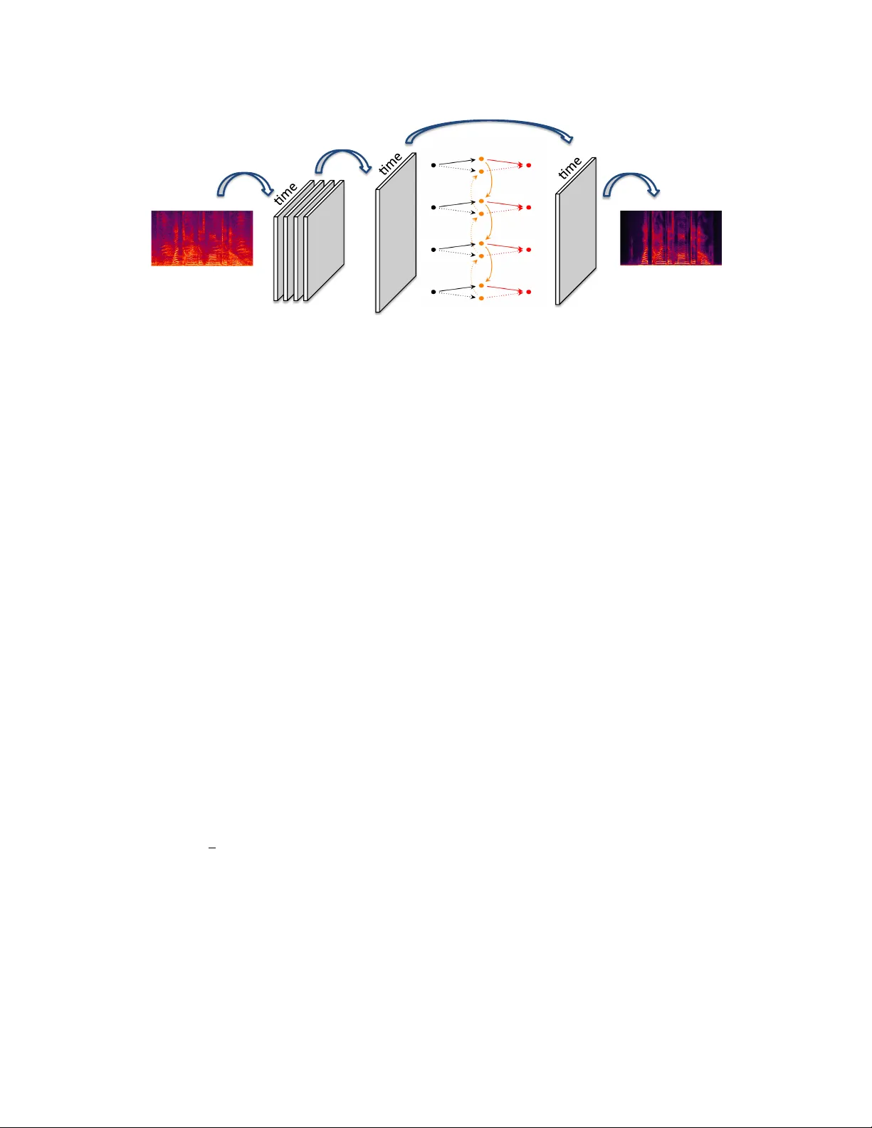
CONV OLUTIONAL-RECURRENT NEURAL NETWORKS FOR SPEECH ENHANCEMENT Han Zhao † Shuayb Zarar ? Ivan T ashev ? Chin-Hui Lee ‡ † Machine Learning Department, Carnegie Mellon Uni versity , Pittsb urgh, P A, USA ? Microsoft Research, One Microsoft W ay , Redmond, W A, USA ‡ School of Electrical and Computer Engineering, Georgia Institute of T echnology , Atlanta, GA, USA ABSTRA CT W e propose an end-to-end model based on con volutional and recurrent neural netw orks for speech enhancement. Our model is purely data-driv en and does not mak e an y assumptions about the type or the stationarity of the noise. In contrast to existing methods that use multilayer perceptrons (MLPs), we employ both con volutional and recurrent neural network architectures. Thus, our approach allows us to exploit local structures in both the frequency and temporal domains. By incorporating prior knowledge of speech signals into the design of model structures, we build a model that is more data-efficient and achiev es better generalization on both seen and unseen noise. Based on e xperiments with synthetic data, we demonstrate that our model outperforms existing methods, improving PESQ by up to 0.6 on seen noise and 0.64 on unseen noise. Index T erms — con volutional neural networks, recurrent neural networks, speech enhancement, regression model 1. INTR ODUCTION Speech enhancement [ 1 , 2 ] is one of the corner stones of b uild- ing robust automatic speech recognition (ASR) and communi- cation systems. The problem is of especial importance no wa- days where modern systems are often b uilt using data-driven approaches based on lar ge scale deep neural networks [ 3 , 4 ]. In this scenario, the mismatch between clean data used to train the system and the noisy data encountered when deploying the system will often degrade the recognition accuracy in practice, and speech enhancement algorithms work as a preprocessing module that help to reduce the noise in speech signals before they are fed into these systems. Speech enhancement is a classic problem that has attracted much research efforts for sev eral decades in the community . By making assumptions on the nature of the underlying noise, statistical based approaches, including the spectral subtrac- tion method [ 5 ], the minimum mean-square error log-spectral method [ 6 ], etc., can often obtain analytic solutions for noise suppression. Howe ver , due to these unrealistic assumptions, most of these statistical-based approaches often fail to build The work was done when HZ was an intern at Microsoft Research. estimators that can well approximate the complex scenarios in real-world. As a result, additional noisy artifacts are usually introduced in the recov ered signals [7]. Related W ork . Due to the av ailability of high-quality , large-scale data and the rapidly growing computational re- sources, data-dri ven approaches using regression-based deep neural networks hav e attracted much interests and demon- strated substantial performance improvements o ver traditional statistical-based methods [ 8 , 9 , 10 , 11 , 12 ]. The general idea of using deep neural networks, or more specifically , the MLPs for noise reduction is not new [ 13 , 14 ], and dates back at least to [ 15 ]. In these works, MLPs are applied as general nonlin- ear function approximators to approximate the mapping from noisy utterance to its clean version. A multiv ariate regression- based objecti ve is then optimized using numeric methods to fit model parameters. T o capture the temporal nature of speech signals, pre vious works also introduced recurrent neural net- works (RNNs) [ 16 ], which remov es the needs for the explicit choice of context windo w in MLPs. Contributions . W e propose an end-to-end model based on con volutional and recurrent neural networks for speech enhancement, which we term as E H N E T . E H N E T is purely data-driv en and does not make any assumptions about the underlying noise. It consists of three components: the con- volutional component exploits the local patterns in the spec- trogram in both frequency and temporal domains, followed by a bidirectional recurrent component to model the dynamic correlations between consecutiv e frames. The final component is a fully-connected layer that predicts the clean spectrograms. Compared with existing models such as MLPs and RNNs, due to the sparse nature of con volutional kernels, E H N E T is much more data-efficient and computationally tractable. Furthermore, the bidirectional recurrent component allo ws E H N E T to model the dynamic correlations between consecu- tiv e frames adaptiv ely , and achie ves better generalization on both seen and unseen noise. Empirically , we ev aluate the ef- fectiv eness of E H N E T and compare it with state-of-the-art methods on synthetic dataset, sho wing that E H N E T achiev es the best performance among all the competitors on all the 5 metrics. Specifically , our model leads up to a 0.6 impro vement of PESQ measure [ 17 ] on seen noise and 0.64 improvement on unseen noise. frequency) feature) feature) convolu/on) concatena/on) bidirec/onal)RNN) regression) Fig. 1 : Model architecture. E H N E T consists of three components: noisy spectrogram is first con volved with kernels to form feature maps, which are then concatenated to form a 2D feature map. The 2D feature map is further transformed by a bidirectional RNN along the time dimension. The last component is a fully-connected netw ork to predict the spectrogram frame-by-frame. E H N E T can be trained end-to-end by defining a loss function between the predicted spectrogram and the clean spectrogram. 2. MODELS AND LEARNING In this section we introduce the proposed model, E H N E T , in detail and discuss its design principles as well as its inductive bias toward solving the enhancement problem. At a high lev el, we view the enhancement problem as a multivariate regression problem, where the nonlinear regression function is parametrized by the network in Fig. 1. Alternatively , the whole network can be interpreted as a complex filter for noise reduction in the frequency domain. 2.1. Problem Formulation Formally , let x ∈ R d × t + be the noisy spectrogram and y ∈ R d × t + be its corresponding clean version, where d is the di- mension of each frame, i.e., number of frequency bins in the spectrogram, and t is the length of the spectrogram. Giv en a training set D = { ( x i , y i ) } n i =1 of n pairs of noisy and clean spectrograms, the problem of speech enhancement can be for- malized as finding a mapping g θ : R d × t + → R d × t + that maps a noisy utterance to a clean one, where g θ is parametrized by θ . W e then solve the follo wing optimization problem to find the best model parameter θ : min θ 1 2 n X i =1 || g θ ( x i ) − y i || 2 F (1) Under this setting, the key is to find a parametric family for denoising function g θ such that it is both rich and data-efficient. 2.2. Con volutional Component One choice for the denoising function g θ is vanilla multilayer perceptrons, which has been extensi vely e xplored in the past few years [ 8 , 9 , 10 , 11 ]. Ho wever , despite being uni versal func- tion approximators [ 18 ], the fully-connected network structure of MLPs usually cannot exploit the rich patterns existed in spectrograms. For e xample, as we can see in Fig. 1, signals in the spectrogram tend to be continuous along the time dimen- sion, and they also hav e similar values in adjacent frequency bins. This ke y observ ation moti vates us to apply con volutional neural networks to efficiently and cheaply extract local patterns from the input spectrogram. Let z ∈ R b × w be a con volutional kernel of size b × w . W e define a feature map h z to be the conv olution of the spectro- gram x with kernel z , follo wed by an elementwise nonlinear mapping σ : h z ( x ) = σ ( x ∗ z ) . Throughout the paper , we choose σ ( a ) = max { a, 0 } to be the rectified linear function (ReLU), as it has been extensi vely verified to be effecti ve in alleviating the notorious gradient v anishing problem in prac- tice [ 19 ]. Each such con volutional kernel z will produce a 2D feature map, and we apply k separate con volutional kernels to the input spectrogram, leading to a collection of 2D feature maps { h z j ( x ) } k j =1 . It is worth pointing out that without padding, with unit stride, the size of each feature map h z ( x ) is ( d − b + 1) × ( t − w + 1) . Howe ver , in order to recover the original speech signal, we need to ensure that the final prediction of the model hav e exactly the same length in the time dimension as the input spectrogram. T o this end, we choose w to be an odd integer and apply a zero-padding of size d × b w / 2 c at both sides of x before con volution is applied to x . This guarantees that the feature map h z ( x ) has t + 2 × b w/ 2 c − w + 1 = t + w − 1 − w + 1 = t time steps, matching that of x . On the other hand, because of the local similarity of the spectrogram in adjacent frequenc y bins, when con volving with the kernel z , we propose to use a stride of size b/ 2 along the frequency dimension. As we will see in Sec. 3, such design will greatly reduce the number of parameters and the computation needed in the following recurrent component, without losing any prediction accurac y . Remark . W e conclude this section by emphasizing that the application of con volution kernels is particularly well suited for speech enhancement in the frequency domain: each kernel can be understood as a nonlinear filter that detects a specific kind of local patterns existed in the noisy spectrograms, and the width of the kernel has a natural interpretation as the length of the context windo w . On the computational side, since con- volution layer can also be understood as a special case of fully- connected layer with shared and sparse connection weights, the introduction of con volutions can thus greatly reduce the computation needed by a MLP with the same expressi ve power . 2.3. Bidirectional Recurrent Component T o automatically model the dynamic correlations between ad- jacent frames in the noisy spectrogram, we introduce bidirec- tional recurrent neural networks (BRNN) that have recurrent connections in both directions. The output of the con volutional component is a collection of k feature maps { h z j ( x ) } k j =1 , h z j ( x ) ∈ R p × t . Before feeding those feature maps into a BRNN, we need to first transform them into a 2D feature map: H ( x ) = [ h z 1 ( x ); . . . ; h z k ( x )] ∈ R pk × t In other words, we v ertically concatenate { h z j ( x ) } k j =1 along the feature dimension to form a stacked 2D feature map H ( x ) that contains all the information from the previous conv olu- tional feature map. In E H N E T , we use deep bidirectional long short-term memory (LSTM) [ 20 ] as our recurrent component due to its ability to model long-term interactions. At each time step t , given input H t : = H t ( x ) , each unidirectional LSTM cell computes a hidden representation − → H t using its internal gates: i t = s ( W xi H t + W hi − → H t − 1 + W ci c t − 1 ) (2) f t = s ( W xf H t + W hf − → H t − 1 + W cf c t − 1 ) (3) c t = f t  c t − 1 + i t  tanh( W xc H t + W hc − → H t − 1 ) (4) o t = s ( W xo H t + W ho − → H t − 1 + W co c t ) (5) − → H t = o t  tanh( c t ) (6) where s ( · ) is the sigmoid function,  means elementwise product, and i t , o t and f t are the input gate, the output gate and the forget gate, respectiv ely . The hidden representation ˜ H t of bidirectional LSTM is then a concatenation of both − → H t and ← − H t : ˜ H t = [ − → H t ; ← − H t ] . T o build deep bidirectional LSTMs, we can stack additional LSTM layers on top of each other . 2.4. Fully-connected Component and Optimization Let ˜ H ( x ) ∈ R q × t be the output of the bidirectional LSTM layer . T o obtain the estimated clean spectrogram, we apply a linear regression with truncation to ensure the prediction lies in the nonnegati ve orthant. Formally , for each t , we hav e: ˆ y t = max { 0 , W ˜ H t + b W } , W ∈ R d × q , b W ∈ R d (7) As discussed in Sec. 2.1, the last step is to define the mean- squared error between the predicted spectrogram ˆ y and the clean one y , and optimize all the model parameters simulta- neously . Specifically , we use AdaDelta [ 21 ] with scheduled learning rate [22] to ensure a stationary solution. 3. EXPERIMENTS T o demonstrate the effectiv eness of E H N E T on speech en- hancement, we created a synthetic dataset, which consists of 7,500, 1,500 and 1,500 recordings (clean/noisy speech) for training, v alidation and testing, respecti vely . Each recording is synthesized by con volving a randomly selected clean speech file with one of the 48 room impulse responses a vailable and adding a randomly selected noise file. The clean speech cor- pus consists of 150 files containing ten utterances with male, female, and children voices. The noise dataset consists of 377 recordings representing 25 different types of noise. The room impulse responses were measured for distances between 1 and 3 meters. A secondary noise dataset of 32 files, with noises that do not appear in the training set, is denoted UnseenNoise and used to generate another test set of 1,500 files. The randomly generated speech and noise le vels provide signal-to-noise ra- tio between 0 and 30 dB. All files are sampled with 16 kHz sampling rate and stored with 24 bits resolution. 3.1. Dataset and Setup As a preprocessing step, we first use STFT to extract the spec- trogram from each utterance. The spectrogram has 256 fre- quency bins ( d = 256) and ∼ 500 frames ( t ≈ 500) frames. T o throughly measure the enhancement quality , we use the fol- lowing 5 metrics to e valuate dif ferent models: signal-to-noise ratio (SNR, dB), log-spectral distortion (LSD), mean-squared- error on time domain (MSE), word error rate (WER, % ), and the PESQ measure. T o measure WER, we use the DNN- based speech recognizer , described in [ 23 ]. The system is kept fixed (not fine-tuned) during the experiment. W e compare our E H N E T with the following state-of-the-art methods: 1. M S . Microsoft’ s internal speech enhancement sys- tem used in production, which uses a combination of statistical-based enhancement rules. 2. D N N - S Y M M [ 9 ]. D N N - S Y M M contains 3 hidden lay- ers, all of which have 2048 hidden units. It uses a symmetric context windo w of size 11. 3. D N N - C AU S A L [ 11 ]. Similar to D N N - S Y M M , D N N - C AU S A L contains 3 hidden layers of size 2048, but instead of symmetric context window , it uses causal context windo w of size 7. 4. R N N - N G [ 16 ]. R N N - N G is a recurrent neural network with 3 hidden layers of size 500. The input at each time step cov ers frames in a context window of length 3. T able 1 : Experimental results on synthetic dataset with both seen and unseen noise, e valuated with 5 dif ferent metrics. Noisy Speech corresponds to the scores obtained without enhancement, while Clean Speech corresponds to the scores obtained using the ground truth clean speech. For each metric, the model achie ves the best performance is highlighted in bold. Seen Noise Unseen Noise Model SNR LSD MSE WER PESQ SNR LSD MSE WER PESQ Noisy Speech 15.18 23.07 0.04399 15.40 2.26 14.78 23.76 0.04786 18.4 2.09 M S 18.82 22.24 0.03985 14.77 2.40 19.73 22.82 0.04201 15.54 2.26 D N N - S Y M M 44.51 19.89 0.03436 55.38 2.20 40.47 21.07 0.03741 54.77 2.16 D N N - C AU S A L 40.70 20.09 0.03485 54.92 2.17 38.70 21.38 0.03718 54.13 2.13 R N N - N G 41.08 17.49 0.03533 44.93 2.19 44.60 18.81 0.03665 52.05 2.06 E H N E T 49.79 15.17 0.03399 14.64 2.86 39.70 17.06 0.04712 16.71 2.73 Clean Speech 57.31 1.01 0.00000 2.19 4.48 58.35 1.15 0.00000 1.83 4.48 (a) Noisy speech. (b) M S . (c) D N N . (d) R N N . (e) E H N E T . (f) Clean speech. Fig. 2 : Noisy and clean spectrograms, along with the denoised spectrograms using different models. The architecture of E H N E T is as follows: the con volutional component contains 256 kernels of size 32 × 11 , with stride 16 × 1 along the frequency and the time dimensions, respec- tiv ely . W e use two layers of bidirectional LSTMs following the conv olution component, each of which has 1024 hidden units. T o train E H N E T , we fix the number of epochs to be 200, with a scheduled learning rate { 1 . 0 , 0 . 1 , 0 . 01 } for e very 60 epochs. For all the methods, we use the validation set to do early stopping and sav e the best model on validation set for ev aluation on the test set. E H N E T does not overfit, as both weight decay and dropout hurt the final performance. W e also experiment with deeper E H N E T with more layers of bidi- rectional LSTMs, b ut this does not significantly impro ve the final performance. W e also observe in our experiments that reducing the stride of con volution in the frequency dimension does not significantly boost the performance of E H N E T , b ut greatly incurs additional computations. 3.2. Results and Analysis Experimental results on the dataset is sho wn in T able 1. On the test dataset with seen noise, E H N E T consistently outperforms all the competitors with a lar ge margin. Specifically , E H N E T is able to impro ve the perceptual quality (PESQ measure) by 0.6 without hurting the recognition accuracy . This is very sur- prising as we treat the underlying ASR system as a black box and do not fine-tune it during the experiment. As a comparison, while all the other methods can boost the SNR ratio, they often decrease the recognition accuracy . More surprisingly , E H N E T also generalizes to unseen noise as well, and it e ven achie ves a larger boost (0.64) on the perceptual quality while at the same time increases the recognition accuracy . T o hav e a better understanding on the experimental result, we do a case study by visualizing the denoised spectrograms from different models. As shown in Fig. 2, M S is the most conservati ve algorithm among all. By not removing much noise, it also keeps most of the real signals in the speech. On the other hand, although D N N -based approaches do a good job in removing the background noise, they also tend to remove the real speech signals from the spectrogram. This explains the reason why D N N -based approaches de grade the recognition accuracies in T able 1. R N N does a better job than D N N , but also fails to k eep the real signals in low frequenc y bins. As a comparison, E H N E T finds a good tradeoff between removing background noise and preserving the real speech signals: it is better than D N N /R N N in preserving high/low-frequenc y bins and it is superior than M S in removing background noise. It is also easy to see that E H N E T produces denoised spectrogram that is most close to the ground-truth clean spectrogram. 4. CONCLUSION W e propose E H N E T , which combines both con volutional and recurrent neural networks for speech enhancement. The in- ductiv e bias of E H N E T makes it well-suited to solv e speech enhancement: the conv olution kernels can efficiently detect local patterns in spectrograms and the bidirectional recurrent connections can automatically model the dynamic correlations between adjacent frames. Due to the sparse nature of conv olu- tions, E H N E T requires less computations than both MLPs and RNNs. Experimental results show that E H N E T consistently outperforms all the competitors on all 5 different metrics, and is also able to generalize to unseen noises, confirming the effecti veness of E H N E T in speech enhancement. 5. REFERENCES [1] Ivan Jele v T ashev , Sound captur e and pr ocessing: prac- tical appr oaches , John Wile y & Sons, 2009. [2] Philipos C Loizou, Speech enhancement: theory and practice , CRC press, 2013. [3] Geoffre y Hinton, Li Deng, Dong Y u, George E Dahl, Abdel-rahman Mohamed, Navdeep Jaitly , Andrew Se- nior , V incent V anhouck e, Patrick Nguyen, T ara N Sainath, et al., “Deep neural networks for acoustic mod- eling in speech recognition: The shared views of four research groups, ” IEEE Signal Pr ocessing Magazine , v ol. 29, no. 6, pp. 82–97, 2012. [4] Dario Amodei, Sundaram Ananthanarayanan, Rishita Anubhai, Jingliang Bai, Eric Battenber g, Carl Case, Jared Casper , Bryan Catanzaro, Qiang Cheng, Guoliang Chen, et al., “Deep speech 2: End-to-end speech recognition in english and mandarin, ” in International Conference on Machine Learning , 2016, pp. 173–182. [5] Stev en Boll, “Suppression of acoustic noise in speech using spectral subtraction, ” IEEE T ransactions on acous- tics, speech, and signal pr ocessing , vol. 27, no. 2, pp. 113–120, 1979. [6] Y ari v Ephraim and David Malah, “Speech enhancement using a minimum mean-square error log-spectral ampli- tude estimator , ” IEEE T ransactions on Acoustics, Speech, and Signal Pr ocessing , vol. 33, no. 2, pp. 443–445, 1985. [7] Amir Hussain, Mohamed Chetouani, Stefano Squartini, Alessandro Bastari, and Francesco Piazza, “Nonlinear speech enhancement: An ov ervie w , ” in Pr ogr ess in non- linear speech pr ocessing , pp. 217–248. Springer , 2007. [8] Xugang Lu, Y u Tsao, Shigeki Matsuda, and Chiori Hori, “Speech enhancement based on deep denoising autoen- coder ., ” in Interspeech , 2013, pp. 436–440. [9] Y ong Xu, Jun Du, Li-Rong Dai, and Chin-Hui Lee, “ An experimental study on speech enhancement based on deep neural networks, ” IEEE Signal pr ocessing letters , vol. 21, no. 1, pp. 65–68, 2014. [10] Y ong Xu, Jun Du, Li-Rong Dai, and Chin-Hui Lee, “ A regression approach to speech enhancement based on deep neural networks, ” IEEE/A CM T ransactions on Au- dio, Speech and Language Processing (T ASLP) , vol. 23, no. 1, pp. 7–19, 2015. [11] Seyedmahdad Mirsamadi and Iv an T ashev , “Causal speech enhancement combining data-dri ven learning and suppression rule estimation., ” in INTERSPEECH , 2016, pp. 2870–2874. [12] Kaizhi Qian, Y ang Zhang, Shiyu Chang, Xuesong Y ang, Dinei Florêncio, and Mark Hasegaw a-Johnson, “Speech enhancement using bayesian wa venet, ” Pr oc. Interspeech 2017 , pp. 2013–2017, 2017. [13] Shinichi T amura, “ An analysis of a noise reduction neural network, ” in Acoustics, Speech, and Signal Pr ocessing, 1989. ICASSP-89., 1989 International Confer ence on . IEEE, 1989, pp. 2001–2004. [14] Fei Xie and Dirk V an Compernolle, “ A family of mlp based nonlinear spectral estimators for noise reduc- tion, ” in Acoustics, Speech, and Signal Pr ocessing, 1994. ICASSP-94., 1994 IEEE International Conference on . IEEE, 1994, vol. 2, pp. II–53. [15] Shin’ichi T amura and Alex W aibel, “Noise reduction using connectionist models, ” in Acoustics, Speech, and Signal Pr ocessing, 1988. ICASSP-88., 1988 International Confer ence on . IEEE, 1988, pp. 553–556. [16] Andrew L Maas, Quoc V Le, T yler M O’Neil, Oriol V inyals, Patrick Nguyen, and Andrew Y Ng, “Recur- rent neural networks for noise reduction in robust asr , ” in Thirteenth Annual Confer ence of the International Speech Communication Association , 2012. [17] ITU-T Recommendation, “Perceptual ev aluation of speech quality (pesq): An objective method for end-to- end speech quality assessment of narrow-band telephone networks and speech codecs, ” Rec. ITU-T P . 862 , 2001. [18] Kurt Hornik, Maxwell Stinchcombe, and Halbert White, “Multilayer feedforward networks are uni versal approx- imators, ” Neural networks , v ol. 2, no. 5, pp. 359–366, 1989. [19] Andrew L Maas, A wni Y Hannun, and Andre w Y Ng, “Rectifier nonlinearities impro ve neural network acoustic models, ” in Pr oc. ICML , 2013, vol. 30. [20] Sepp Hochreiter and Jürgen Schmidhuber , “Long short- term memory , ” Neur al computation , vol. 9, no. 8, pp. 1735–1780, 1997. [21] Matthew D Zeiler , “ Adadelta: an adapti ve learning rate method, ” arXiv pr eprint arXiv:1212.5701 , 2012. [22] Li Deng, Geof frey Hinton, and Brian Kingsb ury , “New types of deep neural network learning for speech recogni- tion and related applications: An ov erview , ” in Acoustics, Speech and Signal Pr ocessing (ICASSP), 2013 IEEE In- ternational Confer ence on . IEEE, 2013, pp. 8599–8603. [23] Frank Seide, Gang Li, and Dong Y u, “Conv ersational speech transcription using context-dependent deep neural networks, ” in T welfth Annual Confer ence of the Interna- tional Speech Communication Association , 2011.