Accurate Sine-Wave Amplitude Measurements Using Nonlinearly Quantized Data

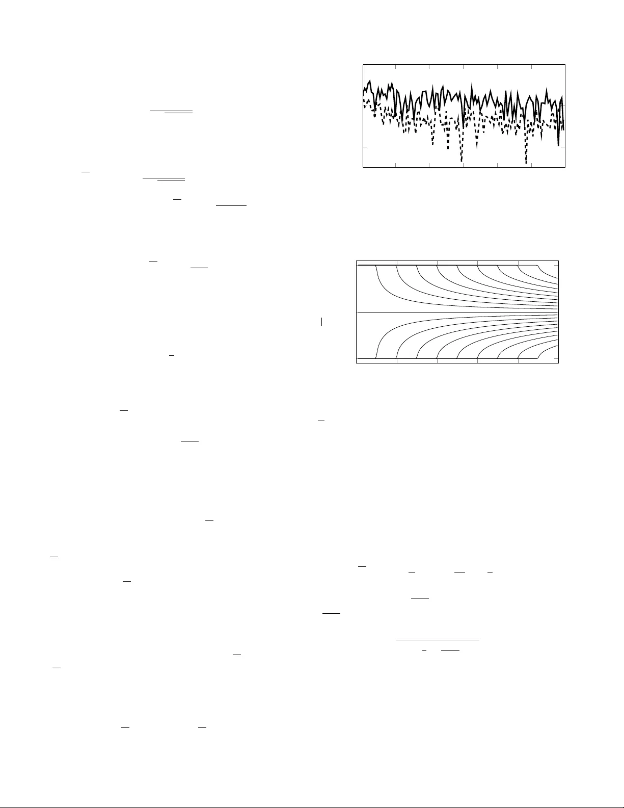
1 Accurate Sine W a v e Amplitude Measurements using Nonlinearly Quantized Data P . Carbone, F ellow Member , IEEE and J. Schoukens, F ellow Member , IEEE and I. Kollar , F ellow Member , IEEE and A. Moschitta Member , IEEE c  2015 IEEE. Personal use of this material is permitted. Permission from IEEE must be obtained for all other uses, in any current or future media, including reprinting/republishing this material for advertising or promotional purposes, creating new collective works, for resale or redistribution to servers or lists, or reuse of any copyrighted component of this work in other works. DOI: 10.1109/TIM.2015.2463331 Abstract —The estimation of the amplitude of a sine wa ve from the sequence of its quantized samples is a typical problem in instrumentation and measurement. A standard appr oach for its solution makes use of a least squares estimator (LSE) that, howe ver , does not perform optimally in the presence of quantization errors. In fact, if the quantization error cannot be modeled as an additive noise source , as it often happens in practice, the LSE r eturns biased estimates. In this paper we consider the estimation of the amplitude of a noisy sine wave after quantization. The proposed technique is based on a uniform distribution of signal phases and it does not requir e that the quantizer has equally spaced transition levels. Experimental results show that this technique removes the estimation bias associated to the usage of the LSE and that it is sufficiently robust with r espect to small uncertainties in the known values of transition levels. Index T erms —Quantization, estimation, nonlinear estimation problems, identification, nonlinear quantizers. I . I N T R O D U C T I O N Almost all modern instruments acquire data by means of Analog–to–Digital Conv erters (ADCs). While technology has progressed to yield ADCs with increasing performance in terms of po wer consumption, effecti ve bits and rate–of– con vergence, the nonlinear transformation implied by the con- version process may still result in inaccurate estimates of input signal parameters. In fact, the majority of results associated to the quantization operation performed by ADCs, are deri ved by assuming a perfectly uniform input–output characteristic, with equally spaced transition levels . When this occurs, the ADC is termed linear with an obvious semantic abuse, giv en that ev en a uniformly spaced stepwise input–output characteristic results in a nonlinear transformation of the input signal. Based on these hypotheses, general properties of quantized signals are deri ved that refer to the analysis of spectra [3]–[5], determination of the ef fect of dithering both in amplitude– and in frequency–domains [7]–[10], application of the quantization theorem [11], analysis of the quantization error probability density function and estimation of the parameters of a sine wa ve using its quantized samples [12], [13]. More ev olved models recognize that ADCs, in practice, are characterized by non–ev enly spaced transition lev els whose P . Carbone and Antonio Moschitta are with the Uni versity of Perugia - Engineering Department, via G. Duranti, 93 - 06125 Perugia Italy , J. Schoukens is with the Vrije Universiteit Brussel, Department ELEC, Pleinlaan 2, B1050 Brussels, Belgium. I. K ollar is with the Budapest Uni versity of T echnology and Economics, Department of Measurement and Information Systems, 1521 Budapest, Hun- gary . value may also v ary depending on usage conditions and en vironmental factors. Fe wer results are available on the char- acteristics of nonlinearly quantized signals. As an e xample, an interesting area of research in this field is represented by meth- ods for the compensation of the input–output characteristics of an ADC to reduce the effects associated to the non–uniform spacing of transition levels [32]. The problem of estimating the amplitude of a sine wave using its quantized samples is relev ant in sev eral engineer- ing applications: for ADC testing purposes [15][16], in the estimation of power quality associated to electrical systems [17], in the characterization of wa veform digitizers [18] and in the measurement of impedances [2], just to name a few . Quantization is always affected by some additiv e noise contributions. The noise may be artificially added, as when dithering is performed [19], or just be the ef fect of input– referred noise sources associated to the behavior of electronic devices. It is known that small amount of additive noise added before quantization may linearize the stepwise input–output characteristics, but that large amount of noise is needed for the linearization of quantizers with non–uniformly distrib uted transition lev els [20]. T o solve this identification problem, the least squares esti- mator (LSE) is often used [21][22]. Ho wev er, the nonlinearity renders the estimator progressiv ely more biased and far from optimal, as the ADC characteristics increasingly departs from uniformity . Previous work on this subject was published in [23], [24] where a general frame work for system identification based on nonlinearly quantized data is described. In [25] a similar approach was used to pro vide estimates of amplitude and initial record phase of a synchr onously sampled sine w ave. In this paper we consider the problem of estimating the amplitude of a noisy sine wave by using quantized samples. Data are considered quantized by a de vice having known transition lev els that are not necessarily uniformly spaced in the signal input range. It will be shown at first that the LSE fails to provide unbiased estimates. Then a new estimator is proposed that does not require coherent sampling nor knowledge of initial record phase as required by the estimator presented in [25]. Simulation and experimental results will be used to show that the new estimator: • removes most of the bias both when the ADC has uniform or non–uniform transition levels; • is capable to estimate the sine w ave amplitude ev en under sev ere quantization (e.g., with a 2 bit ADC) and thus, outperforms the LSE. 2 Q ( · ) x n ⌘ n y n ✓ Fig. 1. The signal chain considered in this paper . I I . S I G N A L S A N D S Y S T E M S The signal chain considered in this paper is shown in Fig. 1. In this figure, x n = sin(2 π λn + φ 0 ) n = 0 , . . . , N − 1 (1) represents a known discrete time deterministic sequence with φ 0 as a possibly unkno wn initial record phase, not to be estimated, n the time index and λ = f f s , the normalized sine wa ve frequency , where f is the sine wav e frequency and f s is the sampling rate. Moreo ver , in Fig. 1, θ represents the constant sine wav e amplitude to be estimated, η n is a zero– mean noise sequence with known probability density function (PDF) and statistically independent outcomes. Observe that in this case a basic assumption is that the DC lev el is exactly zero. In Fig. 1, Q ( · ) models the instantaneous effect of the ADC on the signal. It is characterized by ( L − 1) known transition lev els that do not need to be uniformly spaced in the input range, given by the normalized interv al [ − 1 , 1] . If some of the assumed parameters are unknown, e.g. noise variance or threshold levels, they need to be estimated during an initial system calibration phase. Each record, obtained by collecting quantizer output data, contains N samples y n , n = 0 , . . . , N − 1 that are processed by the algorithms analyzed in this paper . Each ADC output sample can accordingly be modeled as a random variable taking values in L possible categories with probability determined by the input sequence, the noise PDF and the ADC transition levels. Assume also that the quantizer output is equal to y [ k ] : = −  L 2 − 1  ∆ + k ∆ , k = 0 , . . . , L − 1 , when its input takes v alues in the interval [ T k , T k +1 ) , where L = 2 b , b is the number of bits, T k is the k –th quantizer transition lev el and ∆ is the quantization step. Observe that if a uniform ADC is considered, T k = −  L − 1 2  ∆ + k ∆ . Accordingly , k = 0 and k = L − 1 correspond to the quantizer output being equal to −  L 2 − 1  ∆ and L ∆ 2 respectiv ely . Also define the quantization error e n = y n − θ x n and consider as negligible the probability that the quantizer input tak es v alues outside the interval [ − 1 , 1] . When the noise standard de viation σ = 0 , this occurs when the sine wave amplitude obeys the bound, θ <  L − 1 2  ∆ . A. Pr oblem Statement W ith the signals and systems defined above, the estimation problem can be set as follo ws: estimate the sine wa ve ampli- 0 . 2 0 . 4 0 . 6 0 . 8 1 0 0 . 2 0 . 4 0 . 6 ( a ) θ estimator bias / ∆ 200 400 600 800 1 , 000 − 1 − 0 . 5 0 0 . 5 ( b ) transition lev el INL / ∆ 0 . 2 0 . 4 0 . 6 0 . 8 1 0 . 2 0 . 4 0 . 6 ( c ) θ estimator bias / ∆ Fig. 2. LSE: Estimation of the amplitude of a noisy sine wa ve quantized with uniform and non–uniform quantizers: (a) LSE estimator bias associated to the usage of a 10 –bit uniform quantizer; (b) INL of a 10 –bit non–uniform quantizer used to obtain data shown in (c); LSE estimator bias associated to the usage of the 10 –bit non–uniform quantizer with the estimated ± 1 σ band, graphed using dashed lines (c). Each sample is obtained by using 100 records of data with N = 2000 and σ = 0 . 3∆ . tude θ using an N –length sequence of samples obtained by quantizing a noisy version of the sinusoidal signal. B. Pr oblem Analysis The problem described in subsection II-A has been cus- tomarily addressed by applying the LSE to the av ailable data. Howe ver , the LSE is not proved to be optimal in the mean–square sense, when data are quantized: estimates may be affected by bias or minimum estimation variance is not attained. A major dif ference occurs if the quantizer is uniform or is not uniform, i.e. if transition lev els are equally and uniformly spread ov er the signal input interval. While reasonable performance is pro vided by LSE when the quantizer is uniform, when integral non–linearity (INL) affects it, traditional estimators become appreciably biased [1]. This means that, on the average, the difference between estimates and θ is no longer ne gligible. T o appreciate this ef fect, consider Fig. 2, where the estimator bias associated to the estimation of θ using an ideally uniform (a) and non–uniform (c) quantizer having INL shown in plot (b), is graphed normalized to ∆ as a function of θ . A 10 –bit monotone quantizer w as assumed and 3 100 records, each containing 2000 samples of input quantized data were used to perform Monte Carlo–based simulations. Zero–mean Gaussian noise ha ving standard deviation equal to 0 . 3∆ was further assumed. Fig. 2(a) shows that when threshold lev els are uniformly spaced, the estimation bias is negligible compared to ∆ . On the contrary when the INL shown in Fig. 2(b) affects the quantizer the bias is no longer negligible with respect to ∆ , as shown by data in Fig. 2(c). Since, in practice, INL almost always af fects the quantizer behavior , it is of interest to propose ne w estimators for θ . The bias associated to the beha vior of the LSE can be explained by observing that the LSE does not include in- formation about the position of the transition lev els, since it only minimizes a figure–of–merit based on the sum of squared errors. Thus, impro vements in estimation performance can be obtained by including also information about INL when processing data. Recall that noise superimposed on the input signal may act as a dither signal, linearizing the behavior of the quantizer and thus rendering the LSE closer to optimality when assum- ing uniform quantizers. Howe ver , when the quantizer is not uniform, the linearization effect induced by small–amplitude dithering is not ef fective, as in this case dithering smooths the input–output characteristics only locally and not over large input intervals [7][10]. Thus, only a large increase in the noise standard deviation would ha ve positiv e effects on the estimator bias shown in Fig. 2(c), at the expense of a large estimator variance and of a higher risk of overloading the ADC. In the next section it is shown ho w to exploit information on the INL and thus on the position of the quantizer transition lev els to remove estimator bias. Solutions differ whether • samples are collected in a small number of groups: this case was treated in [25]; • samples co ver the phase space densely: the simplified approach tak en in [25] cannot be adopted and a ne w estimator is presented here that is based on the ev aluation of statistical moments. I I I . A M E A N V A L U E – B A S E D E S T I M ATO R ( M V B E ) Observe that each output sample carries some information about the parameter to be estimated. In fact by taking into consideration that for a giv en time index n and noise sample η n the ADC output is determined by the input value being lower or lar ger than each transition level, for all transition lev els we can define the indicator variables: z n,k =    1 θ x n + η n > T k n = 0 , . . . , N − 1 k = 0 , . . . , L − 1 0 otherwise (2) Thus, z n,k is a Bernoulli random variable with probability of success p n,k = 1 − F ( T k − θ x n ) , where F ( · ) represents the noise cumulativ e distribution function. The summation of z n,k ov er the entire set of samples av ailable over time provides, Z N ,k = N − 1 X n =0 z n,k (3) that is random variable taking v alues in [0 , N ] . Observe that Z N ,k is not a binomial random v ariable, because the success probability v aries from sample to sample, as x n in the event in (2) depends on the time index n . Notice also that a single instance of (3) is an estimator of the mean value of Z N ,k , that can formally be written as: E ( Z N ,k ) = N − 1 X n =0 E ( z n,k ) = N − 1 X n =0 [1 − F ( T k − θ sin(2 π λn + φ 0 ))] = N − 1 X n =0  1 − F  T k − θ sin  2 π  λn + φ 0 2 π  (4) where E ( · ) is the expectation operator and h·i is the fractional part operator . This expression relates the value of the unknown parameter θ to E ( Z N ,k ) . If the coef ficient of variation of E ( Z N ,k ) is not too lar ge, by the law of large numbers E ( Z N ,k ) can be estimated by a single instance of (3) and the in version of (4) could provide a value of θ once an estimate of E ( Z N ,k ) is av ailable and all other parameters are known. The numerical in version of (4) becomes cumbersome when the number of samples increases significantly and requires kno wledge of both λ and φ 0 , when σ > 0 . In the next subsection it will be shown how to remove both limitations and ho w to obtain a good approximation when σ ' 0 . A. An Approximation of (4) Both the in version of (4) when N becomes large and the necessity of kno wing λ and φ 0 , result in a procedure that is difficult to be applied in practice. While writing a simple exact expression for the sum in (4) appears as a difficult task, a good approximation can be found either by using the Euler– Maclaurin formula [26] or the equidistribution theorem [27]. While the Euler–Maclaurin formula still requires knowledge of λ and φ 0 , the equidistribution theorem states that for any function g ( · ) , and coefficients a and b , with a being irrational , [27]: lim N →∞ 1 N N X n =1 g ( h an + b i ) = Z 1 0 g ( u ) du (5) Thus, when λ is irrational, lim N →∞ 1 N E ( Z N ,k ) = Z 1 0 [1 − F ( T k − θ sin (2 π u ))] du = : E ( Z k ) (6) so that, for suf ficiently lar ge v alues of N , E ( Z k ) can be con- sidered an approximation of E ( Z N,k ) N . Moreover , by defining U as a uniform random variable in [0 , 1] , this term can also be written as E ( Z k ) = E ([1 − F ( T k − θ sin (2 π U ))]) = E (1 − F ( T k − θ X )) (7) 4 where X = sin(2 π U ) is a transformed random variable with a PDF characterized by an arcsin distribution, whose expression is giv en by f X ( x ) =      1 π √ 1 − x 2 − 1 < x < 1 0 otherwise (8) Thus, from (7) we have: E ( Z k ) = Z 1 − 1 1 π √ 1 − x 2 [1 − F ( T k − θ x )] dx (9) When N is sufficiently large, E ( Z k ) ' E ( Z N,k ) N , as defined in (4) where E ( Z N ,k ) is estimated by a single instance of Z N ,k . T o verify this statement, consider the absolute error sequence defined as e ( N , R ) =      E ( Z k ) − 1 N R R X i =1 Z N ,k,i      (10) where R represents the number of records, each containing N samples and Z N ,k,i represents the value of Z N ,k in the i –th record. Expression e ( N , R ) is plotted in Fig. 3 as a function of N = 10 3 , . . . , 120 · 10 3 for R = 10 3 , 5 · 10 4 , when assuming T k = 1 and θ = 1 . Gaussian noise with known variance is assumed so that F ( x ) = Φ  x σ  , where Φ( · ) is the cumulativ e distribution function of a standard Gaussian random variable. It can be observed that for a giv en number of records R , by increasing N , overall lower values of the absolute error are attained. Observe that E ( Z k ) does not depend on φ 0 , the initial record phase, which does not need to be known. For suf- ficiently large values of N , Z N,k N can be made equal to (9) so that the equality can be solved for θ . T o appreciate how the procedure operates, consider the behavior of (9) represented in Fig. 4 as a function of θ , for various values of − 0 . 9 < T k < 0 . 9 and assuming zero–mean Gaussian noise with σ = 1 . 5∆ . For a giv en value of T k , the corresponding curve can be in verted to yield a value for θ once a value on the y –axis is known. The calculation of E ( Z k ) ov er all possible values of k provides such information. Observe that curv es cannot be in verted in 3 cases: when E ( Z k ) = 0 , 0 . 5 , 1 . Thus, the inv ersion procedures discards these values if they are returned by experiments. A special case is the case E ( Z k ) = 0 . 5 . When this occurs there are infinite solutions for θ . This corresponds to the fact that (9) always provides the value 0 . 5 when T k = 0 , independently from the value of θ . Since deri vati ves of the curves in Fig. 4 with respect to θ are close to 0 when the mean value is close to 0 . 5 , to maintain a safety margin that will guarantee possible numerical in version of (9), all v alues of E ( Z k ) such that | E ( Z k ) − 0 . 5 | < 0 . 2 will be discarded, where the threshold 0 . 2 is determined heuristically . By iterating the in version of (9) over all possible values of T k sev eral estimate of θ results. The number of such estimates, defined in the following by M , equals the number of ADC transition lev els, diminished by 1 every time E ( Z k ) = 0 , 1 or | E ( Z k ) − 0 . 5 | < 0 . 2 . The abov e procedure is true for each T k . Thus, we hav e estimates of θ using each transition level. A straightforward combination 0 . 2 0 . 4 0 . 6 0 . 8 1 1 . 2 · 10 5 10 − 7 10 − 5 10 − 3 R = 10 3 R = 5 · 10 4 N | e ( N , R ) | Fig. 3. Absolute value of the approximation error of summation (4) by the integral (7), e ( N , R ) as a function of N , for two values of the number of records R . A single transition value is considered, T k = 1 with θ = 1 . 0 0 . 2 0 . 4 0 . 6 0 . 8 1 0 0 . 5 1 0.1 0.2 0.3 0.4 0.5 0.6 0.7 0.8 0.9 -0.9 -0.8 -0.7 -0.6 -0.5 -0.4 -0.3 -0.2 -0.1 0 θ E ( Z k ) Fig. 4. Behavior of (9) as a function of 0 . 01 < θ < 1 for v arious v alues of − 0 . 9 < T k < 0 . 9 . F or a given value of T k and for a gi ven estimate of E ( Z k ) , the corresponding curv e is numerically inverted to provide a single estimate of θ . of these estimates is their arithmetic mean; a better estimate can be derived by considering the variance of each singular estimate. The general estimation procedure is described by the pseudocode of Algorithm 1 in the table. As a final remark, consider that the solution is much simpler when there is no or very little noise that is when σ ' 0 . In this case F ( · ) can be approximated using a unity step function, so that (9) can be solved to yield: E ( Z k ) ' − 1 π arcsin  T k θ  + 1 2 , σ ' 0 (11) By equating (11) to Z N,k N and solving for θ , when 0 . 2 <    Z N,k N − 0 . 5    < 0 . 5 we have: ˆ θ k ' T k sin h 1 2 − Z N,k N  π i , σ ' 0 (12) When σ is not negligible, (11) is not accurate, since the arcsin function needs to be con volved by the noise PDF . In such cases, a good approximation can be obtained using a T aylor series expansion of the sin/arcsin function. I V . E S T I M ATO R P R O P E RT I E S The properties of the MVBE, as resulting from the solution of (9), were determined both by simulations and measure- 5 Algorithm 1 A procedure for the estimation of θ 1: procedure E S T I M A T O R ( z n,k , T k , λ, φ 0 )  Need all T k ’ s 2: for k ← 0 , L − 1 do  for ev ery transition le vel 3: f or n ← 0 , N − 1 do  for ev ery sample 4: z n,k ← (count of samples > T k ) 5: end f or 6: Z N ,k ← 1 N P N − 1 n =0 z n,k  A count for every k 7: end for 8: M ← 0  now calculate se veral estimates of θ 9: for k ← 0 , L − 1 do  for ev ery count Z N ,k 10: if 0 < Z N ,k < 1 and | Z N ,k − 0 . 5 | > 0 . 2 then 11: g ( θ ) = R 1 − 1 1 π √ 1 − x 2 [1 − F ( T k − θ x )] dx 12: ˆ θ M ← θ such that g ( θ ) = Z N ,k  one estimate 13: M ← M + 1  count the number of estimates 14: end if 15: end for 16: ˆ θ ← 1 M M − 1 X j =0 ˆ θ j  final estimate as the mean v alue 17: retur n ˆ θ 18: end procedure 0 1 , 000 2 , 000 3 , 000 4 , 000 − 10 − 5 0 ( a ) code bin INL/ ∆ 0 0 . 2 0 . 4 0 . 6 0 . 8 1 − 1 0 1 2 ( b ) θ estimator bias/ ∆ LSE new estimator Fig. 5. Simulation results obtained with a monotonous 12 –bit non uniform ADC: (a) INL normalized to ∆ as a function of the code–bin; (b) normalized absolute estimation error as a function of the sine wave amplitude in the case of the LSE and of the MVBE. ments. A. Simulation Results Algorithm 1 was first implemented in C –code using the GNU Scientific Library that was needed for the numerical calculation of the inte gral in (9) and for its in version. A 12 –bit non–uniform ADC was simulated by using a resistor ladder characterized by normally distributed resistance v alues to realize the 2 12 − 1 transition lev els. This approach guarantees monotonicity of the simulated ADC and allo ws values of the INL greater than ∆ . The beha vior of INL normalized to ∆ , is plotted in Fig. 5(a), as a function of the code bin. Sine wa ves with amplitude θ varying between 0 . 05 and 1 were assumed as the input signal, and R = 10 records of N = 32193 samples each were collected and processed with λ = 1050 π / N and σ = 0 . 21∆ . Results obtained by using the LSE and the MVBE are shown in Fig. 5(b), where the estimator bias normalized to ∆ , is plotted for both cases using a solid and a dashed line, respecti vely . It can be observed that the MVBE removes the bias associated to the behavior of the LSE. In this case, the additional error associated to the usage of the simplified version of this estimator provided by (12) is negligible for all practical purposes with the exclusion of very small v alues of θ . In this latter case the number of excited thresholds is limited and ne glecting the effect of noise produces a small detectable difference between the two estimation approaches. Consider that, being based on the kno wledge of the thresh- old le vels, the MVBE is characterized by a ne gligible bias e ven if se vere quantization is performed. T o prove this statement a 2 –bit uniform quantizer w as assumed and the algorithm was applied with parameters: σ = 0 . 12∆ , λ = 0 . 723457 , φ 0 = 0 . 4876 , N = 106777 . The estimator bias in the case of the MVBE and the LSE is shown in Fig. 6. The LSE not being optimal in this case performs very poorly while the MVBE provides a very good performance. Finally , the v ariances of MVBE and LSE were ev aluated against the Cramer–Rao lower bound (CRLB), by assuming an 8 –bit uniform ADC. The CRLB was calculated by the same approach described in [28], without resorting to the simplifying assumption introduced by noise model of quan- tization [11]. V ariances were normalized to the corresponding CRLB as a function of θ / ∆ . Results based on 100 records obtained with σ = 0 . 2∆ and N = 1024 are shown in Fig. 7. Simulations show that because of its bias, the variance of LSE becomes smaller than the CRLB for some values of θ / ∆ . Con versely , MVBE is capable to reduce the bias at the e xpense of a larger than the CRLB variance. B. Experimental Results T o prov e the validity of the MVBE proposed in this paper , experimental results were obtained using the measurement chain depicted in Fig. 8. A rubidium source (Standford Re- search Systems PRS10) controlled the wav eform synthesizer (Agilent 33220A) used to generate the sine wa ve signal fed to a 12 –bit commercial data acquisition board (DA Q, National Instruments NI6008). The instruments were connected to a portable PC using the Ethernet network, while the D A Q 6 0 . 25 0 . 3 0 . 35 0 . 4 0 . 45 0 . 5 0 0 . 1 θ estimator bias/ ∆ LSE new estimator Fig. 6. Simulation results obtained with a monotonous 2 –bit ideally uniform ADC: normalized estimator bias as a function of the sine wa ve amplitude in the case of the LSE and of MVBE ( σ = 0 . 12∆ , λ = 0 . 723457 , φ 0 = 0 . 4876 , N = 106777 ). 0 20 40 60 80 100 120 1 2 3 4 θ / ∆ estimator variance/CRLB ( θ ) new estimator LSE Fig. 7. Simulation results obtained with an 8 –bit ideally uniform ADC: variance of the MVBE and of the LSE normalized to the corresponding CRLB as a function of θ / ∆ ( σ = 0 . 2∆ , λ = 0 . 1234 , N = 1000 ). SYNTHESIZER 6+1/2 DIGIT DMM RUBIDIUM OSCILLA TOR DAQ PC USB IN OUT ETHERNET IN ETHERNET Fig. 8. The measurement set–up used to obtain experimental data. The controlled synthesizer sources a sine wav e to the 12 –bit data acquisition board, whose amplitude is measured by the digital multimeter in A C mode. A PC uses Ethernet and USB to control the measurement chain. −6 −4 −2 0 2 4 6 −5 0 5 ( m e an i /o c ur v e) / ∆ ( DA Q i np u t v o l t a ge ) / ∆ Fig. 9. Normalized mean v alue of the D A Q input/output characteristic as a function of the normalized input v oltage (bold solid line). Shown are also estimated transition voltages normalized to ∆ (thin vertical solid lines). Experimental results are obtained by averaging 2000 records, each based on 1200 DC input voltage values provided by the synthesizer shown in Fig. 8. The input was measured by the DMM in averaging mode, to provide the reference value shown on the x –axis. board was connected using the Universal Serial Bus (USB). A 6 1 / 2 digit multimeter (DMM, Keithle y 8845A) was used as a reference instrument to obtain an accurate value of the generated signal amplitude, giv en that its accuracy is in the order of 0 . 06% of the measurement result in the used measurement range ( 100 mV). This setup was first used to estimate the transition le vels of the ADC embedded in the D A Q and its v oltage gain. The v alues of the transition le vels, normalized to ∆ = 5 . 096 mV are shown in Fig. 9 using thin solid vertical lines. In the same figure it is shown the mean input/output characteristics of the DA Q, obtained by averaging 2000 records of 1200 input voltage values, distrib uted in the interval [ − 0 . 3986 , 0 . 4007] V . The shape of the input/output curve does not show the typical staircase behavior associated to a perfect quantizer because of the smoothing effect of wide–band noise as sho wn in [7], [29]. Observe also that the transition v oltages are not uniformly spaced, thus causing nonlinearity in the quantizer . Also the standard deviation of the equiv alent input–referred noise source σ was determined as being about equal to 0 . 17∆ . It must be observed that a much lar ger value of σ resulted when the screen of the portable PC was used, because of electromagnetic disturbances. The best measurement condition was obtained by using an external monitor . This setup w as then used to collect 3 records of N = 287431 samples of a sine wav e with frequency 99 . 3715 Hz, sampled at a nominal sampling rate equal to 9135 samples per second, so that λ = 0 . 0108781 . . . resulted. Records were taken by varying θ / ∆ in the interval (21 , 52) . In this interval, the magnitudes of the measured INL and DNL of the D A Q were all upper bounded by ∆ / 2 , thus making the ADC very linear . Processing experimental data highlighted ne w issues not previously considered during the modeling phase. Data were processed both by the LSE method resulting in the sine–fit algorithm and by the MVBE. In some cases also data post– processing was performed before applying the LSE. It was observed that: • the 3 –parameter sine–fit algorithm (amplitude, offset and initial record phase) did not perform satisfactorily be- 7 cause of the uncertainties in the determination of λ , primarily due to tolerances in the DA Q sampling rate. Thus, a 4 –parameter sine–fit method was used to also estimate the frequency parameter; • the performance of the sine–fit algorithm in estimating the sine wa ve amplitude depended on whether data were or were not corrected for the effect of the ADC gain that was about equal to 1 . 001 ; since uncompensated data resulted in a worse performance, data were first compensated for the effect of the gain before applying the LSE; • before applying the LSE data could alternatively be post– processed to correct the ADC behavior for the non– uniform distribution of the transition lev el. This was done by applying the midpoint correction technique to raw ADC data [30][31][32]. Accordingly , to the k –th output code was assigned the value 1 2 ( T k + T k +1 ) , with T k , T k +1 being the corresponding code boundary transition levels, so to guarantee that an ideal 45 ◦ line would pass through the centers of all steps in the ADC quantization input– output characteristic [30]. The performance comparison between estimators is sho wn in Fig. 10 where the bias , i.e. the mean error , associated to the usage of both the sine–fit and the MVBE are displayed. Graphs show that the MVBE almost uniformly reduces the bias even in this case, when the magnitude of the INL and DNL of the considered ADC are very small. The difference in performance would be much larger with an ADC with a more se vere nonlinear behavior . Observe also that the MVBE is ev en slightly superior over the 4 –parameter sine fit based on midpoint –corrected data. The ratio between the squared bias summed o ver all records and values of θ is about equal to 0 . 75 , in fav or of the MVBE. This can be explained by the fact that the midpoint correction is optimal according to the Lloyd’ s approach [33], only when the input signal has a PDF that is constant within the quantization bin. This happens, for instance, when the input amplitudes are uniformly distributed as when using a deterministic ramp signal [32]. Observe also that, data post–processing using the midpoint correction would not howe ver be able to remove the effects of coarse quantization, resulting in a poor behavior of the LSE, as shown in Fig. 6. V . C O N C L U S I O N Direct processing of the codes provided by an ADC to estimate parameters associated to ADC input quantities may result in biased estimators, especially when using non uniform quantizers. In this paper we considered the problem of esti- mating the amplitude of a sine wave by means of a set of its samples quantized using a non uniform ADCs. By taking into account knowledge about the actual ADC transition levels it was possible to show that the proposed technique remo ves most of the bias associated to the usage of more traditional estimators such as the leasts square one. Both simulation and experimental results were used to verify the ne w estimator properties under several different values of the noise standard deviation. Observe that only overall statistical information on the signal amplitudes in the form of a probability density 20 25 30 35 40 45 50 − 0 . 1 0 0 . 1 θ / ∆ estimator bias / ∆ sine-fit with gain-only compensation sine-fit with midpoint correction new estimator Fig. 10. Experimental results based on a 12 –bit commercial data acquisition board: estimator bias as a function of the sine wa ve amplitude θ , both normalized to a nominal value ∆ = 5 . 096 mV . Comparison between the performances of the MVBE and of 4 –parameter sine–fit estimator based on gain–compensated or post–processed data. Post–processing is performed using the midpoint correction approach [30][31][32]. Results obtained by averaging 3 records each containing N = 287431 samples obtained at a nominal sine wav e frequency of 99 . 3715 Hz and sampled at a nominal rate of 9135 samples per second. Input noise standard deviation was estimated as 0 . 17∆ . The ADC transition lev els and amplitude gain were estimated in a preceding calibration phase. function was considered by the estimator proposed in this paper . By including also time–related information among input samples and thus using knowledge about the correlation of processed data, further accuracy improvements are expected. The idea presented here can be generalized to other types of input signals and suggests that processing ADC output data by also incorporating kno wledge about the position of the transition lev els provides superior performance o ver the usage of code–domain only approaches. A C K N O W L E D G E M E N T This work was supported in part by the Fund for Scientific Research (FWO-Vlaanderen), by the Flemish Government (Methusalem), the Belgian Government through the Inter univ ersity Poles of Attraction (IAP VII) Program, and by the ERC advanced grant SNLSID, under contract 320378. R E F E R E N C E S [1] P . Carbone, J. Schoukens, “ A Rigorous Analysis of Least Squares Sine Fitting Using Quantized Data: The Random Phase Case, ” IEEE T rans. Instr . Meas. , vol. 63, pp. 512–529, March 2014. [2] P . M. Ramos, M. Fonseca da Silv a, A. Cruz Serra, “Low Frequency Impedance Measurements using Sine–Fitting, ” IMEK O Measurement , 35 (2004), pp. 89–96. [3] R. M. Gray , “Quantization Noise Spectra, ” IEEE Tr ans. Inf. Theory , vol. 36, no. 6, pp. 1220–1244, Nov . 1990. [4] W . R. Bennett, “Spectra of Quantized Signals, ” Bell System technial Journal pp. 446–472, V ol. 27, Issue 3, July 1948. [5] N. M. Blachman, “The intermodulation and distortion due to quantiza- tion of sinusoids, ” IEEE T rans. Acoust., Speech, Signal Processing, vol. ASSP–33, pp. 1417–1426, Dec. 1985. [6] L. Schuchman, “Dither signals and their ef fect on quantization noise, ” IEEE Transaction on Communication T echnology, vol. 12, pp. 162–165, 1964. [7] I. Koll ´ ar , “Bias of mean value and mean square v alue measurement based on quantized data, ” IEEE Tr ans. Instr . Meas. , vol. 43, pp. 373–379, Oct. 1994. [8] R. M. Gray , T . G. Stockham, “Dithered Quantizers, ” IEEE T rans. Inform. Theory , V ol. 39, no. 3, May 1993, pp. 805–812. [9] M. J. Flanagan, G. A. Zimmerman, “Spur–Reduced Digital Sinusoid Synthesis, ” TD A Progess report 42–155, pp. 91–104, Nov . 1993. 8 [10] P . Carbone, D. Petri “Performance of stochastic and deterministic dithered quantizers, ” IEEE T rans. Instr . Meas. , April 2000, vol. 49, no. 2, pp. 337–340. [11] B. W idrow and I. K oll ´ ar , Quantization Noise , Cambridge Univ ersity Press, 2008. [12] D. Petri, D. Bele ga, D. Dallet, Dynamic T esting of Analog-to-Digital Con verters by Means of the Sine–Fitting Algorithms, in Design, Model- ing and T esting of Data Con verters P . Carbone, S. Kiaei, F . Xu, (eds) Berlin: Springer, 2014, pp. 341–377. [13] R. Pintelon, J. Schoukens, “ An improved sine-wave fitting procedure for characterizing data acquisition channels, ” IEEE T rans. Instr . Meas. vol. 45, no. 2, Apr . 1996. [14] H. Lundin, P . Handel, “Look–Up T ables, Dithering and V olterra Series for ADC Improvements, ” in Design, Modeling and T esting of Data Con verters , P . Carbone, S. Kiaei, F . Xu, (eds) Berlin: Springer , 2014, pp. 249–275. [15] IEEE, Standar d for T erminology and T est Methods for Analog–to– Digital Converter s , IEEE Std. 1241, Aug. 2009. [16] J. J .Blair , T . E. Linnenbrink, “Corrected RMS Error and Effectiv e Number of Bits for Sine W av e ADC T ests, ” Computer Standar ds & Interfaces , Elsevier , V ol. 26, pp. 43–49, 2003. [17] L. Cristaldi, A. Ferrero, S. Salicone, “ A Distributed System for Electric Power Quality Measurement, ” IEEE T rans. Instr . Meas. vol. 51, no. 4, pp. 776–781, Aug. 2002. [18] IEEE, Standar d for Digitizing W aveform Recor ders , IEEE Std. 1057, Apr . 2008. [19] Analog De vices, AD9265 Data Sheet Re v C, 08/2013. IMEK O Mea- sur ement , 35 (2004), pp. 89–96. [20] M.F . W agdy , “Effect of Additiv e Dither on the Resolution of ADC?s with Single-Bit or Multibit Errors, ” IEEE T rans. Instr . Meas. , vol. 45, pp. 610–615, April 1996. [21] F . Correa Alegria, “Bias of amplitude estimation using three-parameter sine fitting in the presence of additive noise, ” IMEKO Measurement , 2 (2009), pp. 748–756. [22] P . Handel, “ Amplitude estimation using IEEE-STD-1057 three- parameter sine wav e fit: Statistical distrib ution, bias and variance, ” IMEK O Measurement , 43 (2010), pp. 766–770. [23] L. Y . W ang, G. G. Y in, J. Zhang, Y . Zhao, System Identification with Quantized Observations, Springer Science, 2010. [24] L. Y . W ang and G. Y in, “ Asymptotically efficient parameter estimation using quantized output observations, ” Automatica , V ol. 43, 2007, pp. 1178–1191. [25] P . Carbone, J. Schoukens, A. Moschitta, “Parametric System Identifi- cation Using Quantized Data, ” IEEE T rans. Instr . Meas. accepted for publication. [26] R. L. Graham, D. E. Knuth, O. Patashnik “Concrete Mathematics, 2nd ed., ” Addison W esley Publishing Company , 1995. [27] K. Petersen, Er godic Theory . Cambridge: Cambridge Univ . Press, 1983. [28] P . Carbone, A. Moschitta, “Cramer–Rao lower bound for parametric estimation of quantized sinew aves, ” IEEE T rans. Instr . Meas. , vol. 56, no. 3, pp. 975–982, June 2007. [29] K. Hejn, A. Pacut, “Generalized Model of the Quantization Error – A Unified Approach, ” IEEE Tr ans. Instr . Meas. vol. 45, no. 1, pp. 41–44, Feb . 1996. [30] Y .–C. Jenq, “ A/D Con verters with midpoint correction, ” proc. IEEE Instr . Meas. T ech. Conf. 2003, 20–22 May 2003, pp. 1203–1205 vol. 2, ISSN 1091-5281, DOI: 10.1109/IMTC.2003.1207943. [31] M. Frey , H.–A. Loeliger, “On the Static Resolution of Digitally Cor- rected Analog–to–Digital and Digital–to–Analog Converters With Low- Precision Components, ” IEEE T ransactions on Circuits and Systems I: Re gular P apers , vol. 54, no. 1, pp. 229–237, Jan. 2007, [32] H. Lundin, M. Skoglund, P . H ¨ andel, “Optimal index–bit allocation for dynamic post–correction of analog–to–digital conv erters, ” IEEE T ransactions on Signal Processing , v ol. 53, no. 2, pp. 660–671, Feb. 2005. [33] S. P . Lloyd, “Least squares quantization in PCM, ” IEEE Tr ans. Inf. Theor . , vol. 28, no. 2, pp. 129–137, 1982.