Adversarial Ladder Networks

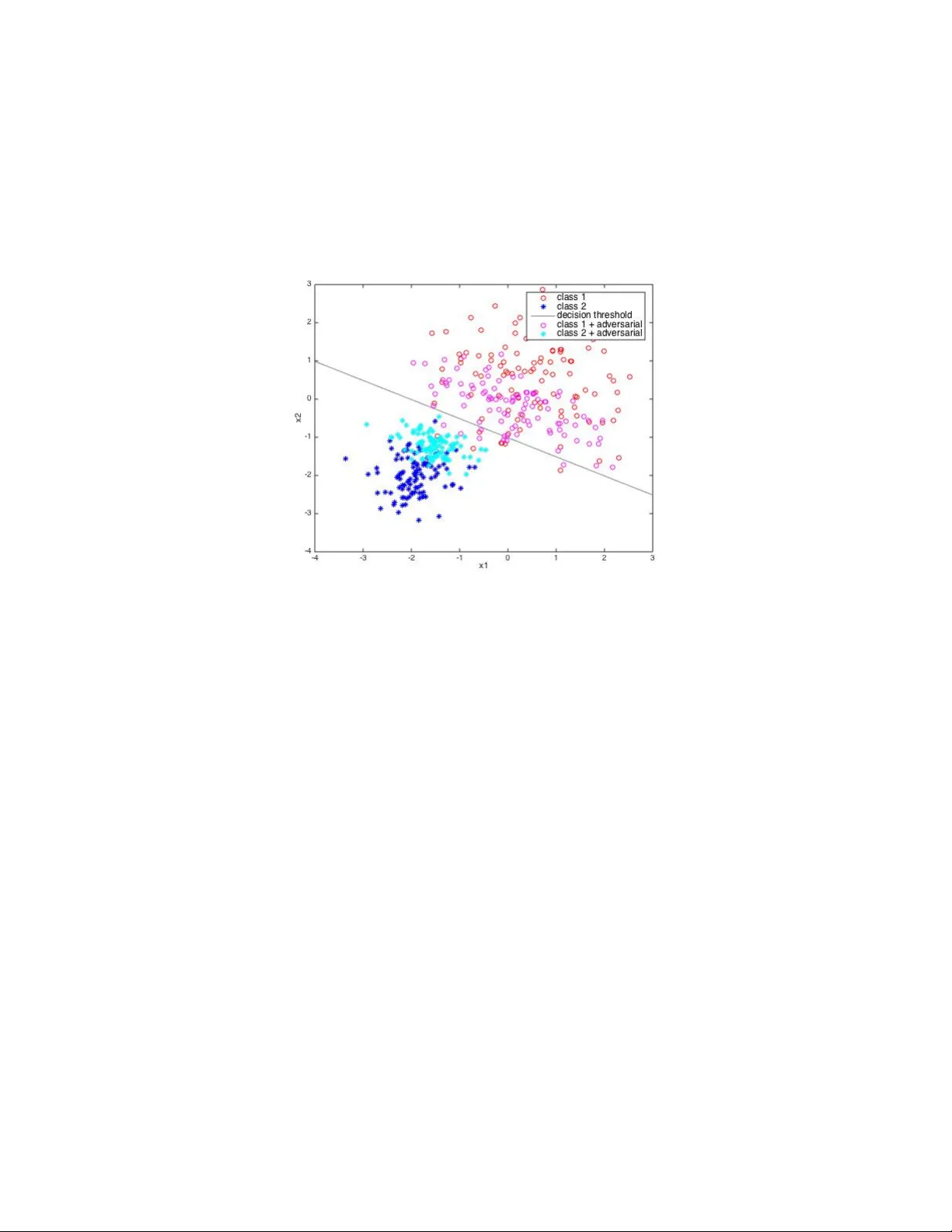
Adv ersarial T raining with Ladder Net w orks Juan Maro ˜ nas Molano jmaronasm@gmail.com 2 , Alb erto Albiol Colomer alalbiol@iteam.up v.es 1 , and Rob erto P aredes Palacios rparedes@dsic.up v.es 2 1 Departamen to de Comunicaciones, Univ ersitat P olit ` ecnica de V al ` encia 2 Departamen to de Sistemas Inform´ aticos y Computaci´ on, Univ ersitat P olit` ecnica de V al ` encia W ednesda y 1 st Marc h, 2017 Abstract The use of unsupervised data in addition to sup ervised data has lead to a significant impro vemen t when training discriminativ e neural net w orks. How ever, the best results w ere ac hieved with a training pro cess that is divided in tw o parts: first an unsup ervised pre-training step is done for initializing the w eights of the netw ork and after these weigh ts are refined with the use of sup ervised data. Recen tly , a new neural net work topology called Ladder Netw ork, where the key idea is based in some prop erties of hierarc hichal latent v ariable mo dels, has b een prop osed as a technique to train a neural netw ork using sup ervised and unsup ervised data at the same time with what is called semi-sup ervised learning. This tec hnique has reac hed state of the art classification. On the other hand adv ersarial noise has impro ved the results of classical sup ervised learning. In this work w e add adversarial noise to the ladder netw ork and get state of the art classification, with several imp ortan t conclusions on how adversarial noise can help in addition with new p ossible lines of inv estigation. W e also prop ose an alternative to add adversarial noise to unsup ervised data. 1 In tro duction Learning unconditional distributions p ( x ) using unsup ervised data can b e useful for learning a neural net- w ork that mo dels a conditional distribution p ( t | x ) where t represents the target of the task. Learning such distributions can b e used to initialize the weigh ts of the net works, using the sup ervised data to refine the parameters and adjust them to the task at hand. This pre-trained neural netw ork has already learnt imp or- tan t features to represent the underlying distribution of the data x . Classical approac hes for learning p ( x ) and use them for then learning p ( t | x ) are under tw o subsets. Deep b elief netw orks [Hin ton and Salakhutdino v, 2006] are based on training pairs of Restricted Boltzmann Ma- c hines (RBM), which are a kind of probabilistic energy-based mo del (EBM) [Lecun et al., 2006][Lecun et al., 2005], and then p erform a finne-tunning of the parameters. Deep b oltzmann machines [Salakhutdino v and Hin ton, 2009] are EBM with more than one hidden lay er to create a deep top ology to after p erform a fine tunning. On the other hand auto encoders [Hinton, 1990] are neural netw orks where the output target is the input. The autoenco der is divided in tw o parts: enco der and deco der. The enco der takes the input x and start reducing the dimensionality where eac h hidden lay er h of the neural netw ork represen ts a dimension. The deco der has the same top ology of the enco der but starts from the last lay er of the enco der (is shared b et ween both parts) and p erform op erations to ha ve an output ¯ x whic h should b e as closed as p ossible to the input. The auto enco der is trained to ac hieve this prop ert y by minimizing the sum of squared error b etw een the input and the reconstruction, as it is assumed the error distribution betw een input and prediction is 1 gaussian. W e then take the pretrained enco der and p erform a finne-tunning of the parameters using sup er- vised data. 2 Semi Sup ervised Learning and Ladder Net w orks Semi sup ervised learning implies learning p ( x ) and p ( t | x ) at the same time. This means using sup ervised and unsupervised data in the same learning pro cedure. The k ey idea of semi sup ervised learning is that unsup ervised learning should find new features that correlates w ell with the already found features suitable for the task. This suitability is driv en by the sup ervised learning pro cedure. Mixing this learning schemes can end up stalling the learning pro cedure for the fact that the targets of the learning schemes are differen t. On one side unsup ervised learning tries to encode all the necessary infor- mation for reconstructing the input. On the other sup ervised learning is more fo cused on finding abstract and inv arian t features (at different lev els of inv ariability) for discriminate the different inputs. Unsup ervised features such as relativ e p osition or size in a face description ma yb e not necessary for a discriminativ e task and discriminative features tipicaly do not hav e information ab out data structure so are unseful to represent x . T o perform semi supervised learning the key idea is that unsupervised learning should b e able of discard information necessary for the reconstruction, and enco de this information in other lay er. F or example sup- p ose sup ervised learning finds useful to ha ve a c haracteristic in a la y er h l where l represen t a particular la yer. A t this level unsup ervised learning needs some kind of representation to keep the reconstruction error lo w and this information is unu seful for supervised learning p erformance. If unsup ervised learning could b e able of represen ting this information in another level l 0 w e could still k eep the reconstruction error low and sup ervised learning could hav e the information needed at this lev el. 2.1 Laten t V ariable Mo dels Laten t v ariable mo dels are mo dels for learning unconditional probability distributions with the particularity that giv en a latent v ariable we can reconstruct the observed v ariable b y means of a lik eliho o d probabilit y distribution. This means the pro ceedure not only depends on h but also on a random pro cedure so in somew ay the model adds their own bits of information for the reconstruction. More formally for a discret distribution: p ( x ) = X ∀ h p ( x | h ) · p ( h ) (1) where p ( x | h ) can b e mo delled like: x = f θ ( h ) + n θ n (2) that is the mean of the likelihoo d distribution is given by the pro jection of h to the observed space and the deviation is giv en b y some noise process. W e can learn the parameters using EM [Dempster et al., 1977]. The main b ottlenec k of EM in some latent v ariable mo dels (like RBM) is that implies computing the p osterior probabilit y p ( h | x ) of the latent v ariable, which is sometimes mathematically intractable. Alternativ es such as sto chastic gradient guided metho ds are used but sometimes implies making approximations using slo w metho ds lik e MCMC exploration. The structure of this mo dels fits well with the semi sup ervised learning paradigm b ecause it allows discard- ing information for the fact that this information can b e someho w added to the reconstruction. Ho w ever a one hidden la yer latent v ariable mo del is unable of discard information because it needs to represen t all the necessary information to represen t p ( x ) in the hidden lay er. The solution is to use hierarchical latent v ariable mo dels where the information can b e somehow distributed b etw een the differen t v ariables and each 2 v ariable is able of adding their own bits of information. The tw o key ideas of this mo dels are that mo delling the observed v ariable as a probability distribution implies that a hidden v ariable can someho w add information (so w e can discard information that is then added) and that making a hierarch y allows information discarding. 2.2 Ladder Net works Ladder Netw ork [V alp ola, 2015] is neural netw ork top ology that implements the key idea of laten t v ariable mo dels that make suitable mixing sup ervised and unsup ervised learning at the same time. The top ology of the netw ork is given by figure 1: Figure 1: Ladder Netw ork T op ology [Ras m us et al., 2015] where as we can see is a kind of auto enco der with lateral connections b etw een the enco der and the deco der, at each level of the netw ork. The deco der reconstruct a v ariable in level ¯ h l using the ab ov e reconstructed v ariable ¯ h l +1 and the corrupted v ariable at the same lev el e h l using a denoising function g ( · , · ). This top ology allo ws information discarding at any level, as long as it is needed. The reconstruction not only dep ends on the level ab ov e (and so dep ends on all the preceding levels) but also on the enco der part. This means their can b e extra added information to the reconstruction (as the latent v ariable mo dels did) and w e can lo ose information at an y level that is enco ded in other levels. Note that with this topology any low er level can b e influence by any signal in an y higher level no matter if it is from the enco der or deco der path. This means that the features the neural net work learns are someho w distributed through the netw ork as long as the sup ervised learning refines which kind of feature need at any level. The minimized cost is given by the expression: C = C s + C u (3) where subindex represent sup ervised and unsup ervised. The sup ervised cost is the cross entrop y , that is (for only one sample X ): C s = − 1 K K X k =1 log P ( e Y k = b Y k | e X ) (4) where K is the lay er dimension and b Y is the target. W e use the corrupted output as the target to regularize. The unsup ervised cost is the weigh ted sum of a reconstruction measure at each level: C u = ω 0 · ( || x − ¯ x || 2 ) 2 + L X l =1 ω d · ( || z l − ¯ z l || 2 ) 2 (5) 3 This unsup ervised cost allows deep arc hitectures b ecause each parameter of the top ology can b e well trained and is difficult to find the gradien t v anishing problem. 2.2.1 Denoising Principle W e should pay sp ecial atten tion to the added noise in the enco der. This noise serv es for tw o purp oses. The first one is implementing the denoising principle of the denoising auto enco der [Vincent et al., 2008][Vincen t et al., 2010] which serves as a go o d regularizator. Noise is also added to force the g ( · , · ) function to use the information in the ab o ve la yer to reconstruct the signal b ecause the signal which minimizes the cost at a lev el l is just h l . This a void the reconstruction function just copy the enco ded signal to the deco der. One more sp ecial thing to remark is that the ladder net work uses batch normalization for tw o purp oses. First is av oid internal cov ariate shift [Ioffe and Szegedy, 2015] and the other is b ecause we hav e to a void the enco der just output constant v alues, as these are the easiest ones to denoise [Rasmus et al., 2015]. 3 Adv ersarial Noise Supp ose w e take a training data X from our distribution. X is an 8-bit normalized image which means there is a precis ion error of 1 255 . No w w e conv ert this image to floating p oin t and add a perturbation τ < 1 2 · 255 . If we then conv ert this new corrupted sample e X = X + τ to an 8-bit image it is clear that X = e X because the p erturbation lies in the same quantification interv al. Our model should correctly classify this sample. [Szegedy et al., 2014] disco ver that neural netw orks are not robust to adversarial examples, that is, examples nearly similar but that highly increase the misclassification error. The first thing w e did is see if the ladder net work w as robust to adversarial examples. F or that reason we trained one mo del which had a 0.51% error on the test set. W e then corrupt the test set with adversarial noise and with random noise ensuring the p o wer from b oth noises was the same. Adv ersarial examples where computed, following [Go o dfellow et al., 2014], like: e X a = X + τ · sign { ∂ C s ∂ x   X } (6) where τ ensures the p erturbation  is under the quan tification error. This fast computing methods can b e deriv ed from a first order T aylor series approximation of C s ( x +  ), see c hapter 1 from [W arde-F arley and Go odfellow, 2017]. Note that the energy of the adversarial noise is τ · K where K is the input dimension and we can corrupt a sample using random gaussian noise like: e X r = X + τ · sign { q } (7) where q is a samples of dimensionality K drawn from a zero mean gaussian distribution N (0 , I ). The p ow er of these noises is the same and is τ · K . The next figure shows a sample of the MNIST test set corrupted with b oth t yp es of noise. As w e see we cannot say which sample will supp ose a higher missclassification error. But we can see the differences in the test error. W e conclude the ladder netw ork is not robust to adv ersarial examples. 4 (a) X a . Error p ercen tage 6.87% (b) X r . Error p ercen tage 0.61% 3.1 Computation of Adversarial Noise Adv ersarial examples can b e generated in several wa ys. An exp ensiv e wa y to generate adversarial examples is by b ox-constrained L-BFGS [Szegedy et al., 2014]. A fast wa y , call the fast gradient metho d [Go o dfellow et al., 2014], compute adversarial examples adding the sign of the deriv ative of the cost function resp ect to the input, following equation 6. This corresp ond to the solution of a maximization problem whose details can b e found in [W arde-F arley and Go odfellow, 2017]. The solution of the problem ensures ||  || ∞ < τ . In this work we explore another wa y of doing this. W e generate adversarial noise following the next equation (we will refer to norm adv ersarial): e X = X + τ a · ∂ C s ∂ x   X ;     ∂ C s ∂ x   X     2 = 1 (8) Note that setting the norm of the gradient v ector to b e one we are also ensuring ||  || ∞ < τ b ecause the norm of this vector is upper-b ounded by the norm of the sign gradient. The norm of the sign gradien t is K 1 2 where K represen t the dimension of that particular lay er. By setting different τ v alues for the tw o differen t noise computation w e can hav e adversarial noise with similar p o wers. F or the MNIST case the sign adversarial noise would hav e a 784 norm v alue and that means the norm adversarial p ow er is one magnitud order b elow the sign adversarial. W e will see that this wa y of computing adv ersarial noise makes sense for three reasons. First one is b ecause in the hyperparameter that sets the p ow er of adversarial noise w e first lo ok for parameters changing only the magnitud order. The second one relies on the intuitiv e idea b ehind adding the gradient of the cost function resp ect to the input. Note that if we add the gradient, which is by definition the direction where the cost maximally c hanges resp ect to an input to that cost, w e are adding a p erturbation whic h directly increase the cost. How ever if we p erform a sign operation we are afecting the phase of this vector and we are not exactly adding the adversarial noise in the gradient direction. The last one will make sense after reading the next subsection but it is directly related to the preceding reason. Basically relies on how can we improv e the p erformance of minimizing the MSE cost function. 3.2 Unsup ervised Adversarial Noise It is clear that the adversarial noise is focus on meausuring how robust a discriminativ e netw ork is to lit- tle p erturbations in sensible directions guided by the target of our task. This is the reason for computing adv ersarial examples using the deriv ativ e of the sup ervised cost, apart from the mathematics exp osed in [W arde-F arley and Go o dfellow, 2017] in tuitiv ely w e add a p erturbation in the direction in whic h the cost highly increase. Adversarial noise is then applied to purely sup ervised learning. Ho wev er we can easily add adversarial noise to unsup ervised data taking the argmax {·} of the softmax out- put and use it as the true tag for that sample. It is clear that in the first steps of the optimization pro cess that tag would b e far from the true tag and that means the adversarial noise will not push to wards the direction in whic h the cost is increase. This technique has already b een prop osed in [Miyato et al., 2016] 5 but with a different ob jective. [Miy ato et al., 2016] prop ose a new ob jectiv e function based on the Kullback Leibler divergence of the clean and corrupted virtual adversarial V A distribution. In this work we generate unsup ervised adversarial, UA, noise following this approac h and add it to the unsup ervised samples. This means adv ersarial noise will in somew ay resem ble gaussian noise in the early training stages. But as long as the netw ork is w ell trained the adv ersarial noise will push the samples to wards the decision b ound. W e can see this in figure 3. Figure 3: This figure represents tw o sup ervised data sets (dark red, circles, and dark blue,stars) drawn from t wo 2D gaussian distributions and the decision b ound. W e hav e applied adversarial noise to b oth data set computing the light red and light blue datasets. As w e can see b oth data sets are pushed to wards the decision b ound and thus tow ards eac h other. In this case we present a sup ervised data set to motiv ate our idea for unsup ervised data. As we see samples correctly classified are pushed tow ards the decision threshold. W e train adding UA noise to force the net work learn to denoise samples in sensible directions. This means extracting features to represent p ( x ) biasing in somew ay ho w we w ant our net work to represent that distribution. The k ey is extract features that correlates with ones find by the sup ervised task reinforcing the learning in the sensible direction. On the other hand, bad classified samples are also pushed tow ards the decision threshold, and that means they are pushed tow ards the data set they b elong to. This is an effect p ossibly present when adding gaussian noise. Note that it makes more sense to add the normalized adversarial noise, as it keeps go o d information ab out the phase of the gradient vector so we are exactly pushing the samples tow ards the worst direction. 3.3 Multila y er Adv ersarial Noise One k ey thing has not b een explored is the computation of adversarial noise at each level of the hierarch y . Understanding this concept is simple, as it only require to compute the deriv ative of the cost resp ect to the input of each lay er x l . Ho wev er, this highly increase the cost of each forw ard-backw ard op eration in the training pro ceedure. T o understand this, consider the input to a L -lay er neural net work. In this case w e need 2 · L op erations b et ween la yers to compute the gradient of the cost resp ect to the input and 2 · L to p erform the parameter up date. It is clear that we cannot compute the gradient resp ect to each input in the same forward-bac kward op eration b ecause in the final forward-bac kward, once we hav e add the adv ersarial noise to the previous lay er, the adv ersarial noise of the next lay er w ould not longer b e the exact deriv ative respect to that input as we 6 compute it with an input c oming from a clean pro jection. Consider the input to the net work x and the input to the first lay er, x 1 = A{ W · x + b } , where A{·} rep- resen ts the non-linear op eration such as the rectifier linear unit. The adv ersarial noise resp ect to the input could b e computed as in equation 6 and the same operation holds for the adversarial resp ect to x 1 . How- ev er b ecause of the relation b etw een x 1 and x once we add some kind of p erturbation to x , the deriv ative resp ect to x 1 c hanges and thus do the adversarial noise. This implies p erforming 2 · ( L − l ) b etw een lay er op erations (BN,drop out,matrix pro duct, vector addition, activ ation function...) to add adv ersarial noise to a particular lay er. So for a L la yer netw ork w e w ould need 2 · L + L P l =0 [2 · L − l ] to perform one minibatch up date. Ho wev er, we can appro ximate this by simply computing the adv ersarial noise in the first forward backw ard. When ha ving saturating non-linearities lik e the sigmoid function, our h yp othesis is that the result is the same as computing it correctly b ecause the output of the sigmoid function is basically the same for inputs in the saturated part of the input range. Moreov er, if we use drop out or gaussian noise to regularize we would ha ve to sav e the drop out mask or the generated gaussian noise, add the adversarial noise, and then p erform the parameter up date using the same mask or num b er generation. This could highly increase the memory cost of a p ossible application. A fast approximation is computing the adversarial noise from the clean path and add it to the corrupted path, or computing it in the first feed-forward of the corrupted path and then p erform another corrupted feed-forward adding the adversarial noise and generating new random n umbers. 4 Exp erimen ts W e perform preliminar exp eriments o ver MNIST. F or this dataset we ev aluated a fully connected netw ork with 50, 100, 1000 and all the lab els and a con volutional netw ork with 100 lab elled data. Details on these net works top ologies can b e found in [Rasmus et al., 2015]. 4.1 Exp erimen tal pro ceedure W e ha ve p erform sev eral experiments to v alidate the differen t proposals along the work. F or the h yp erpa- rameter search of eac h experiment what w e ha ve done is ev aluate the test set training a mo del with one random seed and then p erform several exp eriments with different seeds but the hyperparameter chosen with the first seed and rep ort the mean and standard deviation. This is not a goo d wa y to search hyperparam- eters but the high cost of training the ladder net work made us tak e this solution. The co de is av ailable at h ttps://github.com/jmaronas/ where there is an explanation to replicate the different exp eriments (includ- ing the hardware and soft ware resources). This code starts from the co de of the ladder net work, see [Rasmus et al., 2015] for details. Some conclusions are taken from the fully connected exp erimen ts and directly applied to the con volutional mo dels b ecause of the high cost of the conv olutional net work. W e v alidate our h yp othesis by performing exp erimen ts computing the norm and sign adversarial noise. As we will see, normally , the norm adversarial noise fits b etter with the trained mo del. F or h yp erparameter searc hing w e first lo ok for adversarial noise p ow er going from k · 10 0 to k · 10 − 9 k = 1. The b est h yp erparameter is then used to train 10 models with different seeds. If w e get b etter results than the ladder net work we stop, if not, w e refine the k v alue un til we get a goo d result. W e divide the differen t exp eriments in different sections. W e will know go o ver our w ork, reporting the different results and conclusions. 7 4.2 Sup ervised Input Adv ersarial In this first exp eriment w e simply add adversarial noise to the input of the netw ork. W e searc h hyperparam- eters for the fully connected mo del under the next conditions. F or each of this condition we tried b oth the sign and norm adversarial noises. The op erations are related to the lab elled data, that is, the unsup ervised part of the ladder netw ork (computation and optimization) is exactly the same. W e add adversarial noise plus gaussian noise (MN-2), only adv ersarial noise to the input (MN-1) and gaussian to the remaining lay ers (as the noise in the hidden lay ers is used as a regularizator like drop out [Sriv astav a et al., 2014]) and only adv ersarial to lab elled data (MN-1.1), that is, w e take out the gaussian noise addition of the lab elled data. Note that the only metho d that add purerly adversarial noise is the MN-1.1, as the MN-2 and MN-1 are not exactly adversarial for the reasons we exp osed in section 3.3. In general we found that MN-1.1 w ent b etter than MN-1 in all the exp erimen ts except the 50 tag, and that made us sense. How ever we found that this configurations were far from the state of art. W e saw that the MN-2 approac h yield b etter results than the state of art concluding that the ladder netw ork is really sensible to gaussian noise and that we need other regularizator methods such as adding noise and that an approximate wa y of adding adv ersarial noise giv e also go o d results (we did compute the adversarial noise from the clean path). In [Go o dfellow et al., 2014] they use drop out, but do not sp ecify if they sa ve the drop out mask. Saving or not this mask is something to b e explored. The next table shows the results for the fully connected and the conv oluctional net works. In the conv olutional net work we directly explore the MN-2 option. The table show whether w e use the sign (s) or the norm (n) adv ersarial and the factor used: F C MNIST # of lab els 50 (n;10 − 3 ) 100 (n;1 . 5 · 10 − 2 ) 1000 (n;2 · 10 − 7 ) All lab els (s;3 · 10 − 6 ) DBM, Drop out [Sriv astav a et al., 2014] 0.79% Adversarial [Go o dfellow et al., 2014] 0.78% Ladder full [Rasmus et al., 2015] 1.750% ± 0.582 1.111% ± 0.105 0.880% ± 0.075 0.654% ± 0.052 Adv ersarial Ladder full 1.417% ± 0.539 1.110% ± 0.055 0.861% ± 0.071 0.639% ± 0.056 T able 1: Res ults for fully connected MNIST sup ervised Adversarial Con volutional MNIST # of lab els 100 (n;10 − 3 ) Em b edCNN [W eston et al., 2012] 7.75% SWW AE [Zhao et al., 2015] 9.17% Con v-Small, Γ-mo del [Rasmus et al., 2015] 0.938% ± 0.423 Adv ersarial Ladder Γ -mo del 0.884% ± 0.427 T able 2: Res ults for Con volutional MNIST sup ervised Adversarial 4.3 Unsup ervised Adversarial In this subsection we present the experiments with the unsupervised adv ersarial approac h. These experi- men ts are computed with the approximation in the multila yer adversarial computation commented. On one part we only perform one forw ard-backw ard and on the other we compute the adversarial from the clean path. The ob jective of this approach is first sho w if the unsup ervised adversarial help unsup ervised task, such as minimizing the MSE for the previous reason we ha ve exp osed. On the other we see if this virtual adversarial acts as a go o d regularizer and thus the ob jective is see if it can substitute the gaussian noise by adversarial. F or the lab eled data w e compute UA and add it in eac h lay er. T o analyze this we hav e done the next experiments. On one hand to chec k if we can help minimizing the MSE we add UA only to the input of the unlab eled data. On the other we add multila yer adversarial. W e 8 first present the exp erimen ts c hecking if the adversarial can b e used as a regularizer. F or this we chec k to compute the norm and the sign of the gradient in several wa ys: • Fix factor • Drop F actor • Drop F actor plus gaussian noise Fix factor implies setting a fix v alue for τ . W e chec k for the next v alues: 0.05,0.1,0.15,0.3. The drop factor implies dropping the factor in each iteration by defining a normal distribution with standard deviation given b y: 0.05,0.1,0.15,0.3. The reasons for doing this dropping is the next one. Approximatetly the 70% of v alues of a normal distribution lies b et ween [ − σ, σ ]. This means that the norm of a gaussian noise vector is upp er b ounded by r P k σ 2 , where k is the dimension of the vector, in the 60% of the dropp ed v alues (remark that this p ercen tage is in case all the dimensions in the range are exactly | σ | , if they are lo wer the percentage increases.). If w e drop the τ according to this we will created adversarial v ectors similar in p ow er to the ones w e drop when generating gaussian noise. Having a fix v alue for this factor would no b e a go o d candidate for substituting gaussian noise. Moreov er the norm adversarial is more similar to the gaussian vector as the sign adversarial hav e a fix v alue for the elements of the v ector. When p erforming our exp erimen ts we notice sev eral things. The first one is that the ladder net work is better regularized when using drop ed factor vs the fix factor, as we exp ected. Moreov er what b etter regularize is mixing gaussian noise and UA. Note that the adversarial noise push the features tow ards decision b ounds in which the cost is increased and this is the closest in b etw een class b ounds. Ho wev er we can hav e b ounds resp ect to other classes in other directions and pushing to wards that direction can also help the ladder net work extract relev ant features to b etter generalize. On the other hand the exp eriments without gaussian noise where b etter with the sign. This is b ecause when truncating the phase of the adversarial vector we giv e some randomness to this vector and we know that the ladder netw ork is v ery sensible to gaussian noise to p erform goo d (b oth sup ervised and unsup ervised learning). This also matc hes with what w e sa w when mixing UA with Gaussian. How ever the norm adv ersarial goes b etter when w e incorp orate the gauss ian noise. W e also sho w the results of adding UA only to unlab eled samples and same to lab eled samples to c heck how this new wa y of regularize p erform in differen t targets (Cross entrop y vs MSE). W e can get state of art results as shown in the next tables.: F C MNIST # of lab els 50 100 1000 All lab els Ladder full [Rasmus et al., 2015] 1.750% ± 0.582 1.111% ± 0.105 0.880% ± 0.075 0.654% ± 0.052 Adv ersarial Ladder full 1.417% ± 0.539 1.110% ± 0.055 0.861% ± 0.071 0.639% ± 0.056 Unsup ervised Adversarial Ladder full 1.295% ± 0.391 1.096% ± 0.058 0.92% ± 0.086 0.637% ± 0.050 UA unlab eled Ladder full 1.439% ± 0.5652 1.126% ± 0.058 0.922% ± 0.072 0.614% ± 0.028 UA lab eled Ladder full 1.849% ± 0.645 1.131% ± 0.071 0.908% ± 0.082 0.645% ± 0.044 T able 3: Results for fully connected MNIST unsup ervised Adversarial. UA lab eled refers to adding unsu- p ervised adv ersarial only to lab eled samples F C MNIST Unsup ervised Adv ersarial Ladder full (n;0 . 1) (n;0 . 07) (n;0 . 19) (n;0 . 3) UA unlabeled Ladder full (n;0 . 1) (n;0 . 05) (n;0 . 05) (n;0 . 05) UA labeled Ladder full (n;0 . 05) (n;0 . 3) (n;0 . 05) (n;0 . 1) T able 4: Configurations of the adversarial noise addition of the ab ov e table As we can see in the ab o ve table, the results for the 50, 100 and 60000 tags are b etter than the sup ervised adv ersarial framework. Moreov er the 100 tag and 1000 tag needs more refinement as we had to do in sup ervised adv ersarial. 9 Con volutional MNIST # of lab els 100 (n;10 − 3 ) Con v-Small, Γ-mo del [Rasmus et al., 2015] 0.938% ± 0.423 Adv ersarial Ladder Γ -mo del 0.884% ± 0.427 Unsup ervised Adv ersarial Ladder Γ -mo del 0.86% ± 0 T able 5: Res ults for Con volutional MNIST unsup ervised Adversarial The result rep orted for Unsup ervised Adversarial Ladder conv olutional mo del corresp ond only to the result on one seed, as the models for the other one suffer from numeric saturation. This seed model in the sup ervised adv ersarial had a 0.76% accuracy . W e end up this subsection sho wing the results of adding only unsupervised adv ersarial to the input of the unlab eled part of the netw ork. W e explore if the unsup ervised adversarial can help in minimizing the MSE, as the hidden regularization is done with gaussian noise. The next table sho w the results. F or this exp erimen t we did not p erform refinement: F C MNIST # of lab els 50 100 1000 All lab els Ladder full [Rasmus et al., 2015] 1.750% ± 0.582 1.111% ± 0.105 0.880% ± 0.075 0.654% ± 0.052 Adv ersarial Ladder full 1.417% ± 0.539 1.110% ± 0.055 0.861% ± 0.071 0.639% ± 0.056 UA input unlab eled Ladder full DF 1.678% ± 0.555 1.152% ± 0.069 0.914% ± 0.071 0.606% ± 0.043 UA input unlab eled Ladder full FF 1.397% ± 0.485 1.114% ± 0.078 0.885% ± 0.087 0.625% ± 0.042 T able 6: Results for fully connected MNIST unsup ervised Adv ersarial only added to the input of the unla- b eled net work part. FF means fix factor and DF drop factor. 5 Conclusions and F uture W ork W e hav e shown results on adding adversarial noise to the ladder net work, in addition of new p ossibilities for semisup ervised task. One of the key things adversarial helps for is in o verfitted mo del. Moreov er we see ho w unsup ervised adversarial can help semi sup ervised task such as a regularizator with the gaussian noise and p erforming go o d in minimizing the MSE. F or the first case the drop factor framework w ent b etter and for the second was the fix factor. Dropping factor used for regularization m ak e more sense as the generated UA noise is similar in p o wer distribution to the gaussian noise. On the other hand when pushing samples to try and denoise them seams b etter to hav e a fix v alue to take out this v ariation and let the netw ork learn to denoise (remember this p erturbation is in a really sensible direction). Impro ving the results on the 50 tag was easy , we did not p erform fine tunning of the hyperparameters. This w as not the case with the 100 tag. On the other hand the exp eriments with unsupervised adv ersarial did not require hyperparameter search (except some cases), as we can see in the tables. Our first h yp erparameter where chosen taking in account the standard deviation of the gaussian noise. F uture work will b e fo cused in finishing the exp eriment of sup ervised multila y er adversarial and mixing the differen t prop osals of this work. References A. P . Dempster, N. M. Laird, and D. B. Rubin. Maxim um likelihoo d from incomplete data via the em algorithm. JOURNAL OF THE RO Y AL S T A TISTICAL SOCIETY, SERIES B , 39(1):1–38, 1977. I. J. Go o dfellow, J. Shlens, and C. Szegedy . Explaining and harnessing adversarial examples. arXiv pr eprint arXiv:1412.6572 , 2014. G. E. Hinton and R. R. Salakhutdino v. Reducing the dimensionality of data with neural netw orks. Scienc e , 313(5786):504–507, 2006. 10 G. I. Hin ton. In Y. Ko dratoff and R. S. Mic halski, editors, Machine L e arning , chapter Connectionist Learning Pro cedures, pages 555–610. Morgan Kaufmann Publishers Inc., San F rancisco, CA, USA, 1990. ISBN 0- 934613-09-5. URL http://dl.acm.org/citation.cfm?id=120048.120068 . S. Ioffe and C. Szegedy . Batc h normalization: Accelerating deep net work training b y reducing internal co v ariate shift. arXiv pr eprint arXiv:1502.03167 , 2015. Y. Lecun, F. Jie, and J. N. E. L. Com. Loss functions for discriminative training of energy-based models. In In Pr o c. of the 10-th International Workshop on Artificial Intel ligenc e and Statistics (AIStats05 , 2005. Y. Lecun, S. Chopra, R. Hadsell, R. marc’aurelio, and f. Huang. A T utorial on Energy-Based Learning. In G. Bakir, T. Hofman, B. sch¨ olk opf, A. Smola, and B. T ask ar, editors, Pr e dicting Structur e d Data . MIT Press, 2006. T. Miyato, A. M. Dai, and I. Goo dfellow. Adv ersarial training metho ds for semi-sup ervised text classification. arXiv pr eprint arXiv:1605.07725 , 2016. A. Rasm us, H. V alp ola, M. Honk ala, M. Berglund, and T. Raik o. Semi-supervised learning with ladder net work. CoRR , abs/1507.02672, 2015. URL . R. Salakhutdino v and G. E. Hinton. Deep b oltzmann machines. In International Confer enc e on Artificial Intel ligenc e and Statistics (AIST A TS) , volume 1, page 3, 2009. N. Sriv astav a, G. Hin ton, A. Krizhevsky , I. Sutskev er, and R. Salakhutdino v. Drop out: A simple wa y to prev ent neural netw orks from o verfitting. J. Mach. L e arn. R es. , 15(1):1929–1958, Jan. 2014. ISSN 1532-4435. URL http://dl.acm.org/citation.cfm?id=2627435.2670313 . C. Szegedy , W. Zarem ba, I. Sutsk ever, J. Bruna, D. Erhan, I. Go odfellow, and R. F ergus. Intriguing properties of neural netw orks. arXiv pr eprint arXiv:1312.6199 , 2014. H. V alp ola. F rom neural p ca to deep unsup ervised learning. A dv. in Indep endent Comp onent Analysis and L e arning Machines , pages 143–171, 2015. P . Vincent, H. Laro c helle, Y. Bengio, and P .-A. Manzagol. Extracting and comp osing robust features with denoising auto enco ders. In Pr o c e e dings of the 25th International Confer enc e on Machine L e arning , ICML ’08, pages 1096–1103, New Y ork, NY, USA, 2008. ACM. ISBN 978-1-60558-205-4. doi: 10.1145/1390156. 1390294. URL http://doi.acm.org/10.1145/1390156.1390294 . P . Vincent, H. Laro chelle, I. La joie, Y. Bengio, and P .-A. Manzagol. Stac ked denoising auto enco ders: Learning useful represen tations in a deep net w ork with a lo cal denoising criterion. J. Mach. L e arn. R es. , 11: 3371–3408, Dec. 2010. ISSN 1532-4435. URL http://dl.acm.org/citation.cfm?id=1756006.1953039 . D. W arde-F arley and I. Go odfellow. Adv ersarial p erturbations of deep neural netw orks. In T. Hazan, G. P apandreou, and D. T arlow, editors, Perturb ations, Optimization and Statistics , chapter 1. The Mit Press, 2017. J. W eston, F. Ratle, H. Mobahi, and R. Collob ert. Deep learning via semi-sup ervised embedding. In Neur al Networks: T ricks of the T r ade , pages 639–655. Springer Berlin Heidelb erg, 2012. J. Zhao, M. Mathieu, R. Goroshin, and Y. Lecun. Stack ed what-where auto-encoders. arXiv pr eprint arXiv:1506.02351 , 2015. 11