The Parallel Knowledge Gradient Method for Batch Bayesian Optimization

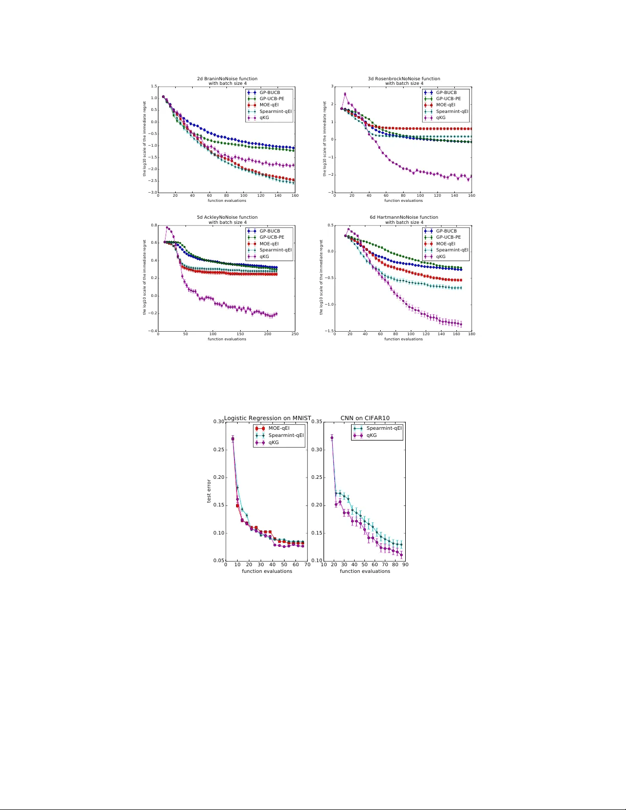
The Parallel Kno wledge Gradient Method f or Batch Bay esian Optimization Jian W u, P eter I. Frazier Cornell Univ ersity Ithaca, NY , 14853 {jw926, pf98}@cornell.edu Abstract In many applications of black-box optimization, one can e valuate multiple points simultaneously , e.g. when ev aluating the performances of several dif ferent neural networks in a parallel computing en vironment. In this paper , we de velop a no vel batch Bayesian optimization algorithm — the parallel knowledge gradient method. By construction, this method provides the one-step Bayes-optimal batch of points to sample. W e provide an efficient strategy for computing this Bayes-optimal batch of points, and we demonstrate that the parallel kno wledge gradient method finds global optima significantly faster than previous batch Bayesian optimization algorithms on both synthetic test functions and when tuning h yperparameters of practical machine learning algorithms, especially when function ev aluations are noisy . 1 Introduction In Bayesian optimization [ 20 ] (BO), we wish to optimize a deriv ati ve-free expensi ve-to-e v aluate function f with feasible domain A ⊆ R d , min x ∈ A f ( x ) , with as fe w function ev aluations as possible. In this paper, we assume that membership in the domain A is easy to ev aluate and we can evaluate f only at points in A . W e assume that e v aluations of f are either noise-free, or hav e additi ve independent normally distrib uted noise. W e consider the parallel setting, in which we perform more than one simultaneous ev aluation of f . BO typically puts a Gaussian process prior distribution on the function f , updating this prior distribution with each ne w observ ation of f , and choosing the next point or points to ev aluate by maximizing an acquisition function that quantifies the benefit of ev aluating the objective as a function of where it is ev aluated. In comparison with other global optimization algorithms, BO often finds “near optimal” function values with fewer e v aluations [ 20 ]. As a consequence, BO is useful when function ev aluation is time-consuming, such as when training and testing complex machine learning algorithms (e.g. deep neural networks) or tuning algorithms on large-scale dataset (e.g. ImageNet) [ 4 ]. Recently , BO has become popular in machine learning as it is highly effecti ve in tuning hyperparameters of machine learning algorithms [8, 9, 20, 23]. Most pre vious work in BO assumes that we e valuate the objecti ve function sequentially [ 13 ], though a few recent papers ha ve considered parallel e v aluations [ 3 , 5 , 18 , 27 ]. While in practice, we can often ev aluate several dif ferent choices in parallel, such as multiple machines can simultaneously train the machine learning algorithm with different sets of hyperparameters. In this paper , we assume that we can access q ≥ 1 ev aluations simultaneously at each iteration. Then we de velop a ne w parallel acquisition function to guide where to ev aluate next based on the decision-theoretical analysis. 30th Conference on Neural Information Processing Systems (NIPS 2016), Barcelona, Spain. Our Contributions. W e propose a novel batch BO method which measures the information gain of e valuating q points via a ne w acquisition function, the parallel kno wledge gradient ( q-KG ). This method is deri ved using a decision-theoretic analysis that chooses the set of points to e valuate ne xt that is optimal in the average-case with respect to the posterior when there is only one batch of points remaining. Naiv ely maximizing q-KG would be extremely computationally intensiv e, especially when q is large, and so, in this paper, we develop a method based on infinitesimal perturbation analysis (IP A) [ 14 ] to ev aluate q-KG ’ s gradient efficiently , allowing its ef ficient optimization. In our e xperiments on both synthetic functions and tuning practical machine learning algorithms, q-KG consistently finds better function values than other parallel BO algorithms, such as parallel EI [ 2 , 20 , 27 ], batch UCB [ 5 ] and parallel UCB with exploration [ 3 ]. q-KG provides especially large v alue when function ev aluations are noisy . The code in this paper is available at https: //github.com/wujian16/Cornell- MOE . The rest of the paper is organized as follows. Section 2 revie ws related work. Section 3 gives background on Gaussian processes and defines notation used later . Section 4 proposes our new acquisition function q-KG for batch BO. Section 5 pro vides our computationally ef ficient approach to maximizing q-KG . Section 6 presents the empirical performance of q-KG and sev eral benchmarks on synthetic functions and real problems. Finally , Section 7 concludes the paper . 2 Related work W ithin the past sev eral years, the machine learning community has revisited BO [ 8 , 9 , 18 , 20 , 21 , 23 ] due to its huge success in tuning hyperparameters of complex machine learning algorithms. BO algorithms consist of two components: a statistical model describing the function and an acquisition function guiding ev aluations. In practice, Gaussian Process (GP) [ 16 ] is the mostly widely used statistical model due to its flexibility and tractability . Much of the literature in BO focuses on designing good acquisition functions that reach optima with as few e valuations as possible. Maximizing this acquisition function usually provides a single point to ev aluate next, with common acquisition functions for sequential Bayesian optimization including probability of improv ement (PI) [ 25 ], expected impro vement (EI) [ 13 ], upper confidence bound (UCB) [ 22 ], entropy search (ES) [ 11 ], and knowledge gradient (KG) [17]. Recently , a few papers ha ve e xtended BO to the parallel setting, aiming to choose a batch of points to ev aluate next in each iteration, rather than just a single point. [ 10 , 20 ] suggests parallelizing EI by iterativ ely constructing a batch, in each iteration adding the point with maximal single-ev aluation EI av eraged ov er the posterior distrib ution of previously selected points. [ 10 ] also proposes an algorithm called “constant liar", which iterativ ely constructs a batch of points to sample by maximizing single- ev aluation while pretending that points previously added to the batch ha ve already returned v alues. There are also work extending UCB to the parallel setting. [ 5 ] proposes the GP-BUCB policy , which selects points sequentially by a UCB criterion until filling the batch. Each time one point is selected, the algorithm updates the kernel function while keeping the mean function fixed. [ 3 ] proposes an algorithm combining UCB with pure exploration, called GP-UCB-PE. In this algorithm, the first point is selected according to a UCB criterion; then the remaining points are selected to encourage the div ersity of the batch. These two algorithms e xtending UCB do not require Monte Carlo sampling, making them fast and scalable. Ho wev er , UCB criteria are usually designed to minimize cumulati ve regret rather than immediate regret, causing these methods to underperform in BO, where we wish to minimize simple regret. The parallel methods abo ve construct the batch of points in an iterati ve greedy fashion, optimizing some single-ev aluation acquisition function while holding the other points in the batch fixed. The acquisition function we propose considers the batch of points collecti vely , and we choose the batch to jointly optimize this acquisition function. Other recent papers that value points collecti vely include [ 2 ] which optimizes the parallel EI by a closed-form formula, [ 15 , 27 ], in which gradient-based methods are proposed to jointly optimize a parallel EI criterion, and [18], which proposes a parallel version of the ES algorithm and uses Monte Carlo sampling to optimize the parallel ES acquisition function. W e compare against methods from a number of these pre vious papers in our numerical experiments, and demonstrate that we provide an impro vement, especially in problems with noisy e v aluations. 2 Our method is also closely related to the knowledge gradient (KG) method [ 7 , 17 ] for the non-batch (sequential) setting, which chooses the Bayes-optimal point to ev aluate if only one iteration is left [ 17 ], and the final solution that we choose is not restricted to be one of the points we ev aluate. (Expected improvement is Bayes-optimal if the solution is restricted to be one of the points we e valuate.) W e go beyond this pre vious work in two aspects. First, we generalize to the parallel setting. Second, while the sequential setting allo ws ev aluating the KG acquisition function exactly , e valuation requires Monte Carlo in the parallel setting, and so we develop more sophisticated computational techniques to optimize our acquisition function. Recently , [ 28 ] studies a nested batch knowledge gradient policy . Howe ver , they optimize ov er a finite discrete feasible set, where the gradient of KG does not exist. As a result, their computation of KG is much less efficient than ours. Moreover , they focus on a nesting structure from materials science not present in our setting. 3 Background on Gaussian pr ocesses In this section, we state our prior on f , briefly discuss well known results about Gaussian processes (GP), and introduce notation used later . W e put a Gaussian process prior over the function f : A → R , which is specified by its mean function µ ( x ) : A → R and kernel function K ( x 1 , x 2 ) : A × A → R . W e assume either e xact or independent normally distributed measurement errors, i.e. the e valuation y ( x i ) at point x i satisfies y ( x i ) | f ( x i ) ∼ N ( f ( x i ) , σ 2 ( x i )) , where σ 2 : A → R + is a known function describing the v ariance of the measurement errors. If σ 2 is not known, we can also estimate it as we do in Section 6. Supposing we have measured f at n points x (1: n ) := { x (1) , x (2) , · · · , x ( n ) } and obtained corre- sponding measurements y (1: n ) , we can then combine these observed function v alues with our prior to obtain a posterior distribution on f . This posterior distribution is still a Gaussian process with the mean function µ ( n ) and the kernel function K ( n ) as follows µ ( n ) ( x ) = µ ( x ) + K ( x , x (1: n ) )  K ( x (1: n ) , x (1: n ) ) + diag { σ 2 ( x (1) ) , · · · , σ 2 ( x ( n ) ) }  − 1 ( y (1: n ) − µ ( x (1: n ) )) , K ( n ) ( x 1 , x 2 ) = K ( x 1 , x 2 ) − K ( x 1 , x (1: n ) )  K ( x (1: n ) , x (1: n ) ) + diag { σ 2 ( x (1) ) , · · · , σ 2 ( x ( n ) ) }  − 1 K ( x (1: n ) , x 2 ) . (3.1) 4 Parallel knowledge gradient ( q-KG ) In this section, we propose a nov el parallel Bayesian optimization algorithm by generalizing the concept of the knowledge gradient from [ 7 ] to the parallel setting. The knowledge gradient policy in [ 7 ] for discrete A chooses the next sampling decision by maximizing the expected incremental value of a measurement, without assuming (as expected impro vement does) that the point returned as the optimum must be a previously sampled point. W e now show how to compute this expected incremental value of an additional iteration in the parallel setting. Suppose that we have observed n function values. If we were to stop measuring now , min x ∈ A µ ( n ) ( x ) would be the minimum of the predictor of the GP . If instead we took one more batch of samples, min x ∈ A µ ( n + q ) ( x ) would be the minimum of the predictor of the GP . The difference between these quantities, min x ∈ A µ ( n ) ( x ) − min x ∈ A µ ( n + q ) ( x ) , is the increment in e xpected solution quality (giv en the posterior after n + q samples) that results from the additional batch of samples. This increment in solution quality is random gi ven the posterior after n samples, because min x ∈ A µ ( n + q ) ( x ) is itself a random vector due to its dependence on the outcome of the sam- ples. W e can compute the probability distrib ution of this difference (with more details gi ven below), and the q-KG algorithm v alues the sampling decision z (1: q ) := { z 1 , z 2 , · · · , z q } according to its expected value, which we call the parallel kno wledge gradient factor , and indicate it using the notation 3 q-KG . Formally , we define the q-KG f actor for a set of candidate points to sample z (1: q ) as q-KG ( z (1: q ) , A ) = min x ∈ A µ ( n ) ( x ) − E n  min x ∈ A µ ( n + q ) ( x ) | z (1: q )  , (4.1) where E n [ · ] := E  ·| x (1: n ) , y (1: n )  is the expectation taken with respect to the posterior distrib ution after n e valuations. Then we choose to ev aluate the next batch of q points that maximizes the parallel knowledge gradient, max z (1: q ) ⊂ A q-KG ( z (1: q ) , A ) . (4.2) By construction, the parallel knowledge gradient policy is Bayes-optimal for minimizing the minimum of the predictor of the GP if only one decision is remaining. The q-KG algorithm will reduce to the parallel EI algorithm if function ev aluations are noise-free and the final recommendation is restricted to the previous sampling decisions. Because under the two conditions above, the increment in expected solution quality will become min x ∈ x (1: n ) µ ( n ) ( x ) − min x ∈ x (1: n ) ∪ z (1: q ) µ ( n + q ) ( x ) = min y (1: n ) − min  y (1: n ) , min x ∈ z (1: q ) µ ( n + q ) ( x )  =  min y (1: n ) − min x ∈ z (1: q ) µ ( n + q ) ( x )  + , which is exactly the parallel EI acquisition function. Howe ver , computing q-KG and its gradient is very e xpensiv e. W e will address the computational issues in Section 5. The full description of the q-KG algorithm is summarized as follows. Algorithm 1 The q-KG algorithm Require: the number of initial stage samples I , and the number of main stage sampling iterations N . 1: Initial Stage: draw I initial samples from a latin hypercube design in A , x ( i ) for i = 1 , . . . , I . 2: Main Stange: 3: for s = 1 to N do 4: Solve (4.2), i.e. get ( z ∗ 1 , z ∗ 2 , · · · , z ∗ q ) = argmax z (1: q ) ⊂ A q-KG ( z (1: q ) , A ) 5: Sample these points ( z ∗ 1 , z ∗ 2 , · · · , z ∗ q ) , re-train the hyperparameters of the GP by MLE, and update the posterior distribution of f . 6: end for 7: retur n x ∗ = argmin x ∈ A µ ( I + N q ) ( x ) . 5 Computation of q-KG In this section, we provide the strategy to maximize q-KG by a gradient-based optimizer . In Section 5.1 and Section 5.2, we describe how to compute q-KG and its gradient when A is finite in (4.1). Section 5.3 describes an effecti ve way to discretize A in (4.1). The readers should note that there are two A s here, one is in (4.1) which is used to compute the q-KG factor giv en a sampling decision z (1: q ) . The other is the feasible domain in (4.2) ( z (1: q ) ⊂ A ) that we optimize over . W e are discretizing the first A . 5.1 Estimating q-KG when A is finite in (4.1) Follo wing [7], we express µ ( n + q ) ( x ) as µ ( n + q ) ( x ) = µ ( n ) ( x ) + K ( n ) ( x, z (1: q ) )  K ( n ) ( z (1: q ) , z (1: q ) ) + diag { σ 2 ( z (1) ) , · · · , σ 2 ( z ( q ) ) }  − 1  y ( z (1: q ) ) − µ ( n ) ( z (1: q ) )  . Because y ( z (1: q ) ) − µ ( n ) ( z (1: q ) ) is normally distributed with zero mean and covariance matrix K ( n ) ( z (1: q ) , z (1: q ) )+ diag { σ 2 ( z (1) ) , · · · , σ 2 ( z ( q ) ) } with respect to the posterior after n observa tions, we can rewrite µ ( n + q ) ( x ) as µ ( n + q ) ( x ) = µ ( n ) ( x ) + ˜ σ n ( x, z (1: q ) ) Z q , (5.1) 4 where Z q is a standard q -dimensional normal random v ector , and ˜ σ n ( x, z (1: q ) ) = K ( n ) ( x, z (1: q ) )( D ( n ) ( z (1: q ) ) T ) − 1 , where D ( n ) ( z (1: q ) ) is the Cholesky factor of the co variance matrix K ( n ) ( z (1: q ) , z (1: q ) ) + diag { σ 2 ( z (1) ) , · · · , σ 2 ( z ( q ) ) } . Now we can compute the q-KG factor using Monte Carlo sam- pling when A is finite: we can sample Z q , compute (5.1), then plug in (4.1), repeat many times and take a verage. 5.2 Estimating the gradient of q-KG when A is finite in (4.1) In this section, we propose an unbiased estimator of the gradient of q-KG using IP A [ 14 ] when A is finite. Accessing a stochastic gradient mak es optimization much easier . By (5.1), we express q-KG as q-KG ( z (1: q ) , A ) = E n  g ( z (1: q ) , A , Z q )  , (5.2) where g = min x ∈ A µ ( n ) ( x ) − min x ∈ A  µ ( n ) ( x ) + ˜ σ n ( x, z (1: q ) ) Z q  . Under the condition that µ and K are continuously differentiable, one can show that (please see details in the supplementary materials) ∂ ∂ z ij q-KG ( z (1: q ) , A ) = E n  ∂ ∂ z ij g ( z (1: q ) , A , Z q )  , (5.3) where z ij is the j th dimension of the i th point in z (1: q ) . By the formula of g , ∂ ∂ z ij g ( z (1: q ) , A , Z q ) = ∂ ∂ z ij µ ( n ) ( x ∗ ( before )) − ∂ ∂ z ij µ ( n ) ( x ∗ ( after )) − ∂ ∂ z ij ˜ σ n ( x ∗ ( after ) , z (1: q ) ) Z q where x ∗ ( before ) = argmin x ∈ A µ ( n ) ( x ) , x ∗ ( after ) = argmin x ∈ A  µ ( n ) ( x ) + ˜ σ n ( x, z (1: q ) ) Z q  , and ∂ ∂ z ij ˜ σ n ( x ∗ ( after ) , z (1: q ) ) =  ∂ ∂ z ij K ( n ) ( x ∗ ( after ) , z (1: q ) )  ( D ( n ) ( z (1: q ) ) T ) − 1 − K ( n ) ( x ∗ ( after ) , z (1: q ) )( D ( n ) ( z (1: q ) ) T ) − 1  ∂ ∂ z ij D ( n ) ( z (1: q ) ) T  ( D ( n ) ( z (1: q ) ) T ) − 1 . Now we can sample man y times and take a verage to estimate the gradient of q-KG via (5.3). This technique is called infinitesimal perturbation analysis (IP A) in gradient estimation [ 14 ]. Since we can estimate the gradient of q-KG ef ficiently when A is finite, we will apply some standard gradient-based optimization algorithms, such as multi-start stochastic gradient ascent to maximize q-KG . 5.3 Appr oximating q-KG when A is infinite in (4.1) through discretization W e have specified ho w to maximize q-KG when A is finite in (4.1), b ut usually A is infinite. In this case, we will discretize A to approximate q-KG , and then maximize over the approximate q-KG . The discretization itself is an interesting research topic [17]. In this paper , the discrete set A n is not chosen statically , but evolv es ov er time: specifically , we suggest drawing M samples from the global optima of the posterior distribution of the Gaussian process (please refer to [ 11 , 18 ] for a description of this technique). This sample set, denoted by A M n , is then e xtended by the locations of pre viously sampled points x (1: n ) and the set of candidate points z (1: q ) . Then (4.1) can be restated as q-KG ( z (1: q ) , A n ) = min x ∈ A n µ ( n ) ( x ) − E n  min x ∈ A n µ ( n + q ) ( x ) | z (1: q )  , (5.4) where A n = A M n ∪ x (1: n ) ∪ z (1: q ) . For the experimental ev aluation we recompute A M n in every iteration after updating the posterior of the Gaussian process. 5 6 Numerical experiments W e conduct experiments in two different settings: the noise-free setting and the noisy setting. In both settings, we test the algorithms on well-known synthetic functions chosen from [ 1 ] and practical problems. Follo wing previous literature [ 20 ], we use a constant mean prior and the ARD Mat ´ e rn 5 / 2 kernel. In the noisy setting, we assume that σ 2 ( x ) is constant across the domain A , and we estimate it together with other hyperparameters in the GP using maximum likelihood estimation (MLE). W e set M = 1000 to discretize the domain follo wing the strategy in Section 5.3. In general, the q-KG algorithm performs as well or better than state-of-the-art benchmark algorithms on both synthetic and real problems. It performs especially well in the noisy setting. Before describing the details of the empirical results, we highlight the implementation details of our method and the open-source implementations of the benchmark methods. Our implementation inherits the open-source implementation of parallel EI from the Metrics Optimization Engine [ 26 ], which is fully implemented in C++ with a python interface. W e reuse their GP regression and GP hyperparameter fitting methods and implement the q-KG method in C++ . The code in this paper is av ailable at https://github.com/wujian16/Cornell- MOE . Besides comparing to parallel EI in [ 26 ], we also compare our method to a well-known heuristic parallel EI implemented in Spearmint [ 12 ], the parallel UCB algorithm (GP-BUCB) and parallel UCB with pure exploration (GP-UCB-PE) both implemented in Gpoptimization [6]. 6.1 Noise-free pr oblems In this section, we focus our attention on the noise-free setting, in which we can e v aluate the objecti ve exactly . W e show that parallel knowledge gradient outperforms or is competitiv e with state-of-the-art benchmarks on sev eral well-known test functions and tuning practical machine learning algorithms. 6.1.1 Synthetic functions First, we test our algorithm along with the benchmarks on 4 well-known synthetic test functions: Branin2 on the domain [ − 15 , 15] 2 , Rosenbrock3 on the domain [ − 2 , 2] 3 , Ackley5 on the domain [ − 2 , 2] 5 , and Hartmann6 on the domain [0 , 1] 6 . W e initiate our algorithms by randomly sampling 2 d + 2 points from a Latin hypercube design, where d is the dimension of the problem. Figure 1 reports the mean and the standard de viation of the base 10 logarithm of the immediate regret by running 100 random initializations with batch size q = 4 . The results sho w that q-KG is significantly better on Rosenbrock3, Ackley5 and Hartmann6, and is slightly worse than the best of the other benchmarks on Branin2. Especially on Rosenbrock3 and Ackley5, q-KG makes dramatic progress in early iterations. 6.1.2 T uning logistic regr ession and con volutional neural networks (CNN) In this section, we test the algorithms on two practical problems: tuning logistic regression on the MNIST dataset and tuning CNN on the CIF AR10 dataset. W e set the batch size to q = 4 . First, we tune logistic re gression on the MNIST dataset. This task is to classify handwritten digits from images, and is a 10 -class classification problem. W e train logistic regression on a training set with 60000 instances with a giv en set of hyperparameters and test it on a test set with 10000 instances. W e tune 4 hyperparameters: mini batch size from 10 to 2000 , training iterations from 100 to 10000 , the ` 2 regularization parameter from 0 to 1 , and learning rate from 0 to 1 . W e report the mean and standard de viation of the test error for 20 independent runs. From the results, one can see that both algorithms are making progress at the initial stage while q-KG can maintain this progress for longer and results in a better algorithm configuration in general. 6 0 20 40 60 80 100 120 140 160 function evaluations −3.0 −2.5 −2.0 −1.5 −1.0 −0.5 0.0 0.5 1.0 1.5 the log10 scale of the immediate regret 2d BraninNoNoise function with batch size 4 GP-BUCB GP-UCB-PE MOE-qEI Spearmint-qEI qKG 0 20 40 60 80 100 120 140 160 function evaluations −3 −2 −1 0 1 2 3 the log10 scale of the immediate regret 3d RosenbrockNoNoise function with batch size 4 GP-BUCB GP-UCB-PE MOE-qEI Spearmint-qEI qKG 0 50 100 150 200 250 function evaluations −0.4 −0.2 0.0 0.2 0.4 0.6 0.8 the log10 scale of the immediate regret 5d AckleyNoNoise function with batch size 4 GP-BUCB GP-UCB-PE MOE-qEI Spearmint-qEI qKG 0 20 40 60 80 100 120 140 160 180 function evaluations −1.5 −1.0 −0.5 0.0 0.5 the log10 scale of the immediate regret 6d HartmannNoNoise function with batch size 4 GP-BUCB GP-UCB-PE MOE-qEI Spearmint-qEI qKG Figure 1: Performances on noise-free synthetic functions with q = 4 . W e report the mean and the standard deviation of the log10 scale of the immediate re gret vs. the number of function ev aluations. 0 10 20 30 40 50 60 70 function evaluations 0.05 0.10 0.15 0.20 0.25 0.30 test error Logistic Regression on MNIST MOE-qEI Spearmint-qEI qKG 10 20 30 40 50 60 70 80 90 function evaluations 0.10 0.15 0.20 0.25 0.30 0.35 CNN on CIFAR10 Spearmint-qEI qKG Figure 2: Performances on tuning machine learning algorithms with q = 4 In the second experiment, we tune a CNN on CIF AR10 dataset. This is also a 10 -class classification problem. W e train the CNN on the 50000 training data with certain hyperparameters and test it on the test set with 10000 instances. For the netw ork architecture, we choose the one in tensorflow tutorial. It consists of 2 con volutional layers, 2 fully connected layers, and on top of them is a softmax layer for final classification. W e tune totally 8 hyperparameters: the mini batch size from 10 to 1000 , training epoch from 1 to 10 , the ` 2 regularization parameter from 0 to 1 , learning rate from 0 to 1 , the kernel size from 2 to 10 , the number of channels in con volutional layers from 10 to 1000 , the number of hidden units in fully connected layers from 100 to 1000 , and the dropout rate from 0 to 1 . W e report the mean and standard deviation of the test error for 5 independent runs. In this example, the q-KG is making better (more aggressi ve) progress than parallel EI e ven in the initial stage and 7 0 20 40 60 80 100 120 140 160 function evaluations −2.5 −2.0 −1.5 −1.0 −0.5 0.0 0.5 1.0 1.5 the log10 scale of the immediate regret 2d Branin function with batch size 4 GP-BUCB GP-UCB-PE MOE-qEI Spearmint-qEI qKG 0 50 100 150 200 250 300 350 function evaluations −2.0 −1.5 −1.0 −0.5 0.0 0.5 1.0 1.5 2.0 2.5 the log10 scale of the immediate regret 3d Rosenbrock function with batch size 4 GP-BUCB GP-UCB-PE MOE-qEI Spearmint-qEI qKG 0 50 100 150 200 250 function evaluations −0.2 0.0 0.2 0.4 0.6 0.8 the log10 scale of the immediate regret 5d Ackley function with batch size 4 GP-BUCB GP-UCB-PE MOE-qEI Spearmint-qEI qKG 0 20 40 60 80 100 120 140 160 180 function evaluations −0.6 −0.4 −0.2 0.0 0.2 0.4 0.6 the log10 scale of the immediate regret 6d Hartmann function with batch size 4 GP-BUCB GP-UCB-PE MOE-qEI Spearmint-qEI qKG Figure 3: Performances on noisy synthetic functions with q = 4 . W e report the mean and the standard de viation of the log10 scale of the immediate regret vs. the number of function ev aluations. maintain this adv antage to the end. This architecture has been carefully tuned by the human expert, and achiev e a test error around 14% , and our automatic algorithm improves it to around 11% . 6.2 Noisy problems In this section, we study problems with noisy function ev aluations. Our results show that the performance gains ov er benchmark algorithms from q-KG evident in the noise-free setting are e ven larger in the noisy setting. 6.2.1 Noisy synthetic functions W e test on the same 4 synthetic functions from the noise-free setting, and add independent gaussian noise with standard de viation σ = 0 . 5 to the function e valuation. The algorithms are not giv en this standard deviation, and must learn it from data. The results in Figure 3 show that q-KG is consistently better than or at least competitiv e with all competing methods. Also observe that the performance advantage of q-KG is larger than for noise-free problems. 6.2.2 Noisy logistic regr ession with small test sets T esting on a large test set such as ImageNet is slow , especially when we must test many times for different h yperparameters. T o speed up hyperparameter tuning, we may instead test the algorithm on a subset of the testing data to approximate the test error on the full set. W e study the performance of our algorithm and benchmarks in this scenario, focusing on tuning logistic regression on MNIST . W e train logistic regression on the full training set of 60 , 000 , but we test the algorithm by testing on 1 , 000 randomly selected samples from the test set, which provides a noisy approximation of the test error on the full test set. 8 0 10 20 30 40 50 60 70 function evaluations 0.05 0.10 0.15 0.20 0.25 0.30 0.35 test error Logistic Regression on MNIST with Smaller Test Sets MOE-qEI Spearmint-qEI qKG Figure 4: T uning logistic regression on smaller test sets with q = 4 W e report the mean and standard deviation of the test error on the full set using the hyperparameters recommended by each parallel BO algorithm for 20 independent runs. The result sho ws that q-KG is better than both v ersions of parallel EI, and its final test error is close to the noise-free test error (which is substantially more e xpensiv e to obtain). As we sa w with synthetic test functions, q-KG ’ s performance advantage in the noisy setting is wider than in the noise-free setting. Acknowledgments The authors were partially supported by NSF CAREER CMMI-1254298, NSF CMMI-1536895, NSF IIS-1247696, AFOSR F A9550-12-1-0200, AFOSR F A9550-15-1-0038, and AFOSR F A9550-16-1- 0046. 7 Conclusions In this paper , we introduce a novel batch Bayesian optimization method q-KG , derived from a decision-theoretical perspectiv e, and dev elop a computational method to implement it efficiently . W e show that q-KG outperforms or is competitiv e with the state-of-the-art benchmark algorithms on sev eral synthetic functions and in tuning practical machine learning algorithms. References [1] D. Bingham. Optimization test problems. http://www.sfu.ca/~ssurjano/optimization. html , 2015. [2] C. Chev alier and D. Ginsbourger . Fast computation of the multi-points expected impro vement with applications in batch selection. In Learning and Intelligent Optimization , pages 59–69. Springer , 2013. [3] E. Contal, D. Buffoni, A. Robicquet, and N. V ayatis. Parallel g aussian process optimization with upper confidence bound and pure exploration. In Machine Learning and Knowledge Discovery in Databases , pages 225–240. Springer , 2013. [4] L. Deng, D. Y u, et al. Deep learning: methods and applications. F oundations and T r ends in Signal Pr ocessing , 7(3–4):197–387, 2014. [5] T . Desautels, A. Krause, and J. W . Burdick. Parallelizing exploration-exploitation tradeoffs in gaussian process bandit optimization. The Journal of Machine Learning Resear ch , 15(1): 3873–3923, 2014. [6] E. C. etal. Gpoptimization. https://reine.cmla.ens- cachan.fr/e.contal/ gpoptimization , 2015. [7] P . Frazier, W . Powell, and S. Dayanik. The knowledge-gradient polic y for correlated normal beliefs. INFORMS journal on Computing , 21(4):599–613, 2009. 9 [8] J. R. Gardner , M. J. Kusner , Z. E. Xu, K. Q. W einberger , and J. Cunningham. Bayesian optimization with inequality constraints. In Pr oceedings of the 31st International Confer ence on Machine Learning (ICML-14) , pages 937–945, 2014. [9] M. Gelbart, J. Snoek, and R. Adams. Bayesian optimization with unkno wn constraints. In Pr o- ceedings of the Thirtieth Conference Annual Confer ence on Uncertainty in Artificial Intelligence (U AI-14) , pages 250–259, Corvallis, Oregon, 2014. A UAI Press. [10] D. Ginsbourger , R. Le Riche, and L. Carraro. Kriging is well-suited to parallelize optimization. In Computational Intelligence in Expensive Optimization Pr oblems , pages 131–162. Springer , 2010. [11] J. M. Hernández-Lobato, M. W . Hoffman, and Z. Ghahramani. Predicti ve entropy search for efficient global optimization of black-box functions. In Advances in Neural Information Pr ocessing Systems , pages 918–926, 2014. [12] R. A. Jasper Snoek, Hugo Larochelle and other Spearmint dev elopers. Spearmint. https: //github.com/HIPS/Spearmint , 2015. [13] D. R. Jones, M. Schonlau, and W . J. W elch. Efficient global optimization of e xpensi ve black-box functions. Journal of Global optimization , 13(4):455–492, 1998. [14] P . L ’Ecuyer . A unified vie w of the IP A, SF, and LR gradient estimation techniques. Management Science , 36(11):1364–1383, 1990. [15] S. Marmin, C. Chev alier, and D. Ginsbour ger . Differentiating the multipoint expected impro ve- ment for optimal batch design. In International W orkshop on Machine Learning, Optimization and Big Data , pages 37–48. Springer , 2015. [16] C. E. Rasmussen. Gaussian pr ocesses for machine learning . MIT Press, 2006. [17] W . Scott, P . Frazier , and W . Powell. The correlated knowledge gradient for simulation optimiza- tion of continuous parameters using gaussian process regression. SIAM J ournal on Optimization , 21(3):996–1026, 2011. [18] A. Shah and Z. Ghahramani. Parallel predictiv e entropy search for batch global optimization of expensi ve objectiv e functions. In Advances in Neural Information Pr ocessing Systems , pages 3312–3320, 2015. [19] S. P . Smith. Differentiation of the cholesky algorithm. Journal of Computational and Gr aphical Statistics , 4(2):134–147, 1995. [20] J. Snoek, H. Larochelle, and R. P . Adams. Practical bayesian optimization of machine learning algorithms. In Advances in neural information pr ocessing systems , pages 2951–2959, 2012. [21] J. Snoek, K. Swersky , R. Zemel, and R. Adams. Input warping for bayesian optimization of non-stationary functions. In Pr oceedings of the 31st International Conference on Machine Learning (ICML-14) , pages 1674–1682, 2014. [22] N. Sriniv as, A. Krause, M. Seeger , and S. M. Kakade. Gaussian process optimization in the bandit setting: No regret and experimental design. In Pr oceedings of the 27th International Confer ence on Machine Learning (ICML-10) , pages 1015–1022, 2010. [23] K. Swersky , J. Snoek, and R. P . Adams. Multi-task bayesian optimization. In Advances in neural information pr ocessing systems , pages 2004–2012, 2013. [24] B. S. Thomson, J. B. Bruckner , and A. M. Bruckner . Elementary r eal analysis . ClassicalReal- Analysis. com, 2008. [25] A. Törn and A. Zilinskas. Global optimization, v olume 350 of lecture notes in computer science, 1989. [26] J. W ang, S. C. Clark, E. Liu, and P . I. Frazier . Metrics optimization engine. http://yelp. github.io/MOE/ , 2014. Last accessed on 2016-01-21. 10 [27] J. W ang, S. C. Clark, E. Liu, and P . I. Frazier . Parallel bayesian global optimization of expensiv e functions. Operations Resear ch , 2015. [28] Y . W ang, K. G. Reyes, K. A. Brown, C. A. Mirkin, and W . B. Powell. Nested-batch-mode learning and stochastic optimization with an application to sequential multistage testing in materials science. SIAM Journal on Scientific Computing , 37(3):B361–B381, 2015. 11 Supplementary Material A Asynchronous q-KG Optimization The (A.1) corresponds to the synchronous q-KG optimization, in which we wait for all q points from our previous batch to finish before searching for a new batch of q points. Howev er , in some applications, we may wish to generate a new batch of points to ev aluate next while p ( < q ) points are still being e valuated, before we hav e their v alues. This is common in training machine learning algorithms, where different machine learning models do not necessarily finish at the same time. max z (1: q ) ⊂ A q-KG ( z (1: q ) , A ) . (A.1) W e can generalize (A.1) to the asynchronous q-KG optimization. Gi ven that p points are still under ev aluation, now we would like to recommend a batch of q points to ev aluate. As we did for the synchronous q-KG optimization abov e, no w we estimate the gradient of the q-KG of the combined q + p points only with respect to the q points that we need to recommend. Then we proceed the same way via gradient-based algorithms. B Speed-up analysis Next, we compare q-KG at dif ferent lev els of parallelism against the fully sequential KG algorithm. W e test the algorithms with different batch sizes on two noisy synthetic functions Branin2 and Hartmann6, whose standard deviation of the noise is σ = 0 . 5 . From the results, our parallel knowledge gradient method does pro vide a speed-up as q goes up. 0 20 40 60 80 100 120 140 160 iterations −2.5 −2.0 −1.5 −1.0 −0.5 0.0 0.5 1.0 1.5 the log10 scale of the immediate regret 2d Branin function qKG, q=1 qKG, q=2 qKG, q=4 qKG, q=8 0 20 40 60 80 100 120 140 160 iterations −0.6 −0.4 −0.2 0.0 0.2 0.4 0.6 the log10 scale of the immediate regret 6d Hartmann function qKG, q=1 qKG, q=2 qKG, q=4 qKG, q=8 Figure 5: The performances of q-KG with different batch sizes. W e report the mean and the standard deviation of the log10 scale of the immediate regret vs. the number of iterations. Iteration 0 is the initial designs. For each iteration later , we ev aluate q points recommended by the q-KG algorithm. C Unbiasedness of the stochastic gradient estimator Recall that in Section 5 of the main document, we hav e expressed the q-KG f actor as follows, q-KG ( z (1: q ) , A ) = E n  g ( z (1: q ) , A , Z q )  (C.1) where the expectation is taken o ver Z q and g ( z (1: q ) , A , Z q ) = min x ∈ A µ ( n ) ( x ) − min x ∈ A  µ ( n ) ( x ) + ˜ σ n ( x, z (1: q ) ) Z q  , ˜ σ n ( x, z (1: q ) ) = K ( n ) ( x, z (1: q ) )( D ( n ) ( z (1: q ) ) T ) − 1 . The main purpose of this section is to prov e the following proposition. 12 Proposition 1. When A is finite, under the condition that µ and K are continuous dif fer entiable, ∂ ∂ z ij q-KG ( z (1: q ) , A )     z (1: q ) = θ (1: q ) = E n  ∂ ∂ z ij g ( z (1: q ) , A , Z q )     z (1: q ) = θ (1: q )  , (C.2) wher e 1 ≤ i ≤ q , 1 ≤ j ≤ d , z ij is the j th dimension of the i th point in z (1: q ) and θ (1: q ) ∈ the interior of A q . W ithout loss of generality , we assume that (1) i and j are fixed in advance and (2) A = [0 , 1] d , we would like to prov e that (C.2) is correct. Before proceeding, we define one more notation f A ,Z q ( z ij ) := g ( z (1: q ) , A , Z q ) where z (1: q ) equals to θ (1: q ) component-wise except for z ij . T o prove it, we cite Theorem 1 in [ 14 ], which requires three conditions to make (C.2) valid: there exists an open neighborhood Θ ⊂ [0 , 1] of θ ij where θ ij is the j th dimension of i th point in θ (1: q ) such that • (i) f A ,Z q ( z ij ) is continuous in Θ for any fix ed A and Z q ; • (ii) f A ,Z q ( z ij ) is differentiable e xcept on a denumerable set in Θ for any gi ven A and Z q ; • (iii) the deriv ativ e of f A ,Z q ( z ij ) (when it exists) is uniformly bounded by Γ( Z q ) for all z ij ∈ Θ , and the expectation of Γ( Z q ) is finite. C.1 Proof of condition (i) Under the condition that the mean function µ and the kernel function K are continuous dif ferentiable, we see that for any gi ven x , ˜ σ n ( x, z (1: q ) ) is continuous dif ferentiable in z (1: q ) by the result that the multiplication, the in verse (when the in verse exists) and the Cholesk y operators preserve continuous differentiability Smith [19] . When A is finite, we see that g ( z (1: q ) , A , Z q ) = min x ∈ A µ ( n ) ( x ) − min x ∈ A  µ ( n ) ( x ) + ˜ σ n ( x, z (1: q ) ) Z q  is continuous in z (1: q ) . Then f A ,Z q ( z ij ) is also continuous in z ij by the definition of the function f A ,Z q ( z ij ) . C.2 Proof of condition (ii) By the expression that f A ,Z q ( z ij ) = min x ∈ A µ ( n ) ( x ) − min x ∈ A  µ ( n ) ( x ) + ˜ σ n ( x, z (1: q ) ) Z q  , if both argmin x ∈ A µ ( n ) ( x ) and argmin x ∈ A  µ ( n ) ( x ) + ˜ σ n ( x, z (1: q ) ) Z q  are unique, then f A ,Z q ( z ij ) is dif ferentiable at z ij . W e define D ( A ) ⊂ Θ to be the set that f A ,Z q ( z ij ) is not dif ferentiable, then we see that D ( A ) ⊂ ∪ x,x 0 ∈ A  z ij ∈ Θ : µ ( n ) ( x ) = µ ( n ) ( x 0 ) , d µ ( n ) ( x ) dz ij 6 = d µ ( n ) ( x 0 ) dz ij  ∪ ∪ x,x 0 ∈ A  z ij ∈ Θ : h x ( z ij ) = h x 0 ( z ij ) , dh x ( z ij ) dz ij 6 = dh x 0 ( z ij ) dz ij  where h x ( z ij ) := µ ( n ) ( x ) + ˜ σ n ( x, z (1: q ) ) Z q . µ ( n ) ( x )  µ ( n ) ( x 0 )  depend on z ij if x = z i ( x 0 = z i ) where z i is the i th point of z (1: q ) . As A is finite, we only need to show that  z ij ∈ Θ : µ ( n ) ( x ) = µ ( n ) ( x 0 ) , d µ ( n ) ( x ) dz ij 6 = d µ ( n ) ( x 0 ) dz ij  and  z ij ∈ Θ : h x ( z ij ) = h x 0 ( z ij ) , dh x ( z ij ) dz ij 6 = dh x 0 ( z ij ) dz ij  is denumerable. Defining η ( z ij ) := h x 1 ( z ij ) − h x 2 ( z ij ) on Θ , one can see that η ( z ij ) is continuous differentiable on Θ . W e would like to show that E := n z ij ∈ Θ : η ( z ij ) = 0 , dη ( z ij ) dz ij 6 = 0 o is denumerable. T o prov e it, we will sho w that E contains only isolated points. Then one can use a theorem in real analysis: any set of isolated points in R is denumerable (see the proof of statement 4.2.25 on page 165 in [ 24 ]). T o prove that E only contains isolated points, we use the definition of an isolated point: y ∈ E is an isolated point of E if and only if x ∈ E is not a limit point of E . W e will prove by contradiction, suppose that y ∈ E is a limit point of E , then it means that there exists a sequence 13 of points y 1 , y 2 , · · · all belong to E such that lim n →∞ y n = z ij . Howe ver , by the definition of deriv ative and η ( y n ) = η ( z ij ) = 0 0 6 = dη ( y ) dy   y = z ij = lim n →∞ η ( y n ) − η ( z ij ) y n − z ij = lim n →∞ 0 = 0 , a contradiction. So we conclude that E only contains isolated points, so is denumerable. Defining δ ( z ij ) := µ ( n ) ( x 1 ) − µ ( n ) ( x 2 ) on Θ , δ ( z ij ) is also continuous differentiable on Θ , then one can similarly prov e that n z ij ∈ Θ : δ ( z ij ) = 0 , dδ ( z ij ) dz ij 6 = 0 o is denumerable. C.3 Proof of condition (iii) Recall from Section 5 of the main document, d dz ij f ( z ij , A , Z q ) = ∂ ∂ z ij g ( z (1: q ) , A , Z q ) = ∂ ∂ z ij µ ( n ) ( x ∗ ( before )) − ∂ ∂ z ij µ ( n ) ( x ∗ ( after )) − ∂ ∂ z ij ˜ σ n ( z (1: q ) , x ∗ ( after )) Z q , where x ∗ ( before ) = argmin x ∈ A µ ( n ) ( x ) , x ∗ ( after ) = argmin x ∈ A  µ ( n ) ( x ) + ˜ σ n ( x, z (1: q ) ) Z q  , and ∂ ∂ z ij ˜ σ n ( z (1: q ) , x ∗ ( after )) =  ∂ ∂ z ij K ( n ) ( x ∗ ( after ) , z (1: q ) )  ( D ( n ) ( z (1: q ) ) T ) − 1 − D ( n ) ( x ∗ ( after ) , z (1: q ) )( D ( n ) ( z (1: q ) ) T ) − 1  ∂ ∂ z ij D ( n ) ( z (1: q ) ) T  ( D ( n ) ( z (1: q ) ) T ) − 1 . W e can calculate the ∂ ∂ z ij µ ( n ) ( x ) as follows ∂ ∂ z ij µ ( n ) ( x ) = ( ∂ ∂ z ij µ ( n ) ( z i ) if x = z i , i.e. the i th point of z (1: q ) 0 otherwise . Using the fact that µ is continuously dif ferentiable and A is compact, then ∂ ∂ z ij µ ( n ) ( x ) is bounded by some B > 0 . By the result that ∂ ∂ z ij ˜ σ n ( z (1: q ) , x ∗ ( after )) is continous, it is bounded by a vector 0 ≤ Λ < ∞ as A is compact. Then     d dz ij f ( z ij , A , Z q )     ≤ 2 B + q X i =1 Λ i | z i | , where Z q = ( z 1 , · · · , z q ) T . And E q X i =1 Λ i | z i | ! = p 2 /π q X i =1 Λ i < ∞ . D Con vergence of stochastic gradient ascent In this section, we will pro ve that stochastic gradient ascent (SGA) con verges to a stationary point. W e follow the same idea of pro ving the Theorem 2 in [27]. First, it requires the step size γ t satisfying γ t → 0 as t → ∞ , P ∞ t =0 γ t = ∞ and P ∞ t =0 γ 2 t < ∞ . Second, it requires the second moment of the gradient estimator is finite. In the above section 1.3, we hav e sho wn that | ∂ ∂ z ij g ( z (1: q ) , A , Z q ) | ≤ 2 B + P q i =1 Λ i | z i | , then E  ∂ ∂ z ij g ( z (1: q ) , A , Z q )  2 ≤ 4 B 2 + q X i =1 Λ 2 i + 4 B p 2 /π q X i =1 Λ i + 4 π X i 6 = j Λ i Λ j < ∞ . 14