Music Genre Classification using Machine Learning Techniques

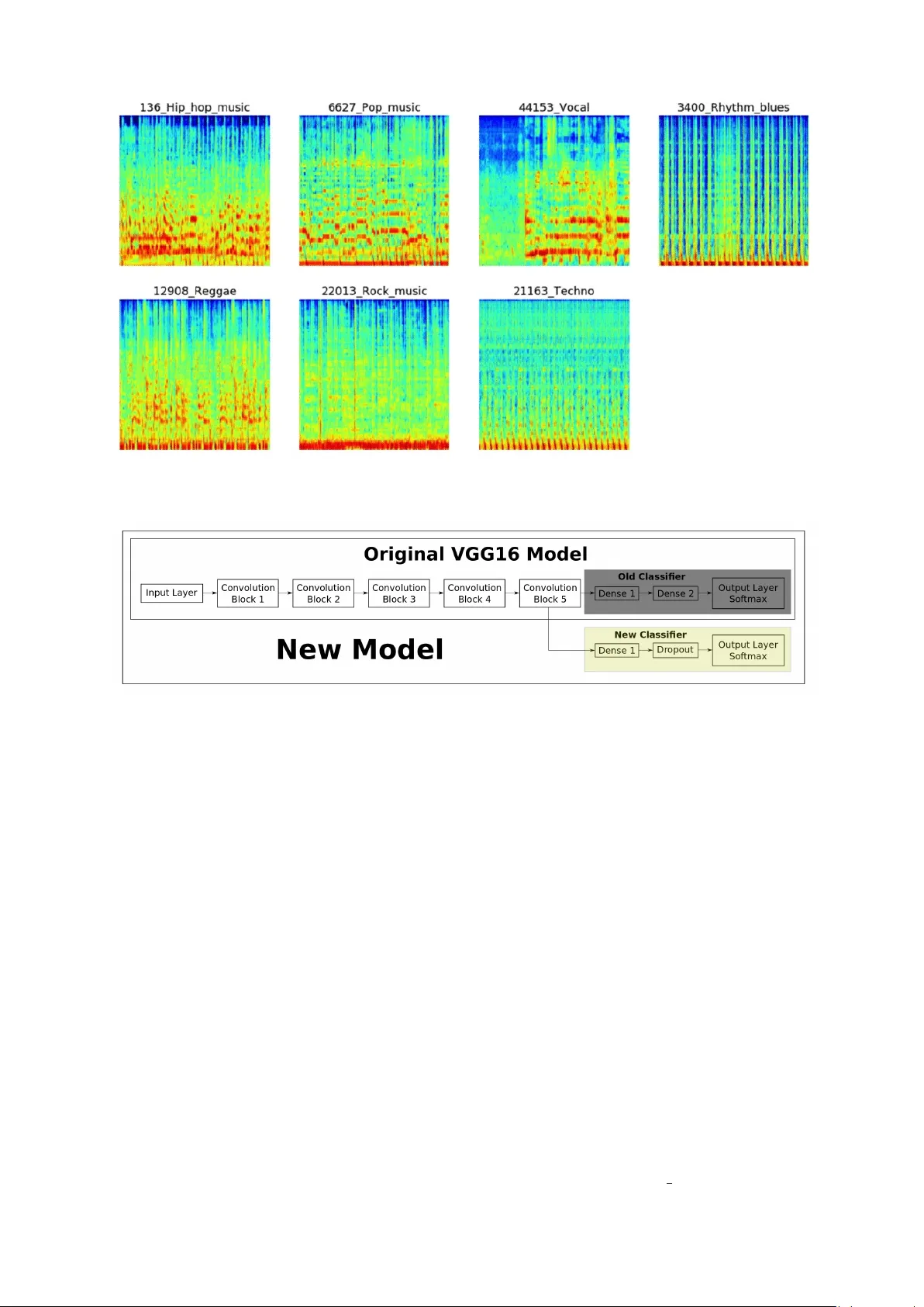
Music Genr e Classification using Machine Learning T echniques Hareesh Bahuleyan Uni versity of W aterloo, ON, Canada hpallika@uwaterloo.ca Abstract Categorizing music files according to their genre is a challenging task in the area of music information retrie v al (MIR). In this study , we compare the performance of two classes of models. The first is a deep learning approach wherein a CNN model is trained end-to-end, to predict the genre label of an audio signal, solely us- ing its spectrogram. The second approach utilizes hand-crafted features, both from the time domain and frequency domain. W e train four traditional machine learning classifiers with these features and compare their performance. The features that con- tribute the most to wards this classification task are identified. The experiments are conducted on the A udio set data set and we report an A UC v alue of 0 . 894 for an en- semble classifier which combines the two proposed approaches. 1 1 Introduction W ith the growth of online music databases and easy access to music content, people find it in- creasing hard to manage the songs that they lis- ten to. One way to cate gorize and organize songs is based on the genre, which is identified by some characteristics of the music such as rhyth- mic structure, harmonic content and instrumen- tation ( Tzanetakis and Cook , 2002 ). Being able to automatically classify and provide tags to the music present in a user’ s library , based on genre, would be beneficial for audio streaming services such as Spotify and iT unes. This study explores the application of machine learning (ML) algo- rithms to identify and classify the genre of a gi v en 1 The code has been opensourced and is available at https://github.com/HareeshBahuleyan/ music- genre- classification audio file. The first model described in this paper uses con volutional neural networks ( Krizhevsky et al. , 2012 ), which is trained end-to-end on the MEL spectrogram of the audio signal. In the sec- ond part of the study , we extract features both in the time domain and the frequency domain of the audio signal. These features are then fed to con- ventional machine learning models nam ely Logis- tic Regression, Random F orests ( Breiman , 2001 ), Gradient Boosting ( Friedman , 2001 ) and Support V ector Machines which are trained to classify the gi ven audio file. The models are ev aluated on the Audio Set dataset ( Gemmeke et al. , 2017 ). W e compare the proposed models and also study the relati ve importance of dif ferent features. The rest of this paper is org anized as follows. Section 2 describes the existing methods in the lit- erature for the task of music genre classification. Section 3 is an overvie w of the the dataset used in this study and how it was obtained. The pro- posed models and the implementation details are discussed in Section 4 . The results are reported in Section 5.2 , followed by the conclusions from this study in Section 6 . 2 Literature Re view Music genre classification has been a widely stud- ied area of research since the early days of the Internet. Tzanetakis and Cook ( 2002 ) addressed this problem with supervised machine learning ap- proaches such as Gaussian Mixture model and k - nearest neighbour classifiers. They introduced 3 sets of features for this task categorized as tim- bral structure, rhythmic content and pitch con- tent. Hidden Marko v Models (HMMs), which hav e been e xtensi vely used for speech recognition tasks, have also been explored for music genre classification ( Scaringella and Zoia , 2005 ; Soltau et al. , 1998 ). Support vector machines (SVMs) with dif ferent distance metrics are studied and compared in Mandel and Ellis ( 2005 ) for classi- fying genre. In Lidy and Rauber ( 2005 ), the authors dis- cuss the contribution of psycho-acoustic features for recognizing music genre, especially the impor - tance of STFT taken on the Bark Scale ( Zwicker and Fastl , 1999 ). Mel-frequency cepstral coef- ficients (MFCCs), spectral contrast and spectral roll-of f were some of the features used by ( Tzane- takis and Cook , 2002 ). A combination of visual and acoustic features are used to train SVM and AdaBoost classifiers in Nanni et al. ( 2016 ). W ith the recent success of deep neural net- works, a number of studies apply these techniques to speech and other forms of audio data ( Abdel- Hamid et al. , 2014 ; Gemmeke et al. , 2017 ). Rep- resenting audio in the time domain for input to neural networks is not very straight-forward be- cause of the high sampling rate of audio signals. Ho we ver , it has been addressed in V an Den Oord et al. ( 2016 ) for audio generation tasks. A com- mon alternati ve representation is the spectrogram of a signal which captures both time and frequency information. Spectrograms can be considered as images and used to train con v olutional neural net- works (CNNs) ( W yse , 2017 ). A CNN was de- veloped to predict the music genre using the raw MFCC matrix as input in Li et al. ( 2010 ). In Lidy and Schindler ( 2016 ), a constant Q-transform (CQT) spectrogram was provided as input to the CNN to achie ve the same task. This work aims to provide a comparative study between 1) the deep learning based models which only require the spectrogram as input and, 2) the traditional machine learning classifiers that need to be trained with hand-crafted features. W e also in v estigate the relativ e importance of different fea- tures. 3 Dataset In this work, we make use of Audio Set , which is a large-scale human annotated database of sounds ( Gemmeke et al. , 2017 ). The dataset was cre- ated by extracting 10-second sound clips from a total of 2.1 million Y ouT ube videos. The audio files hav e been annotated on the basis of an on- tology which co vers 527 classes of sounds includ- ing musical instruments, speech, vehicle sounds, animal sounds and so on 2 . This study requires only the audio files that belong to the music cat- egory , specifically having one of the se v en genre tags sho wn in T able 1 . T able 1: Number of instances in each genre class Genre Count 1 Pop Music 8100 2 Rock Music 7990 3 Hip Hop Music 6958 4 T echno 6885 5 Rhythm Blues 4247 6 V ocal 3363 7 Reggae Music 2997 T otal 40540 The number of audio clips in each cate gory has also been tabulated. The raw audio clips of these sounds hav e not been provided in the A udio Set data release. Ho we ver , the data provides the YouTubeID of the corresponding videos, along with the start and end times. Hence, the first task is to retrie v e these audio files. For the purpose of audio retriev al from Y ouT ube, the following steps were carried out: 1. A command line program called youtube-dl ( Gonzalez , 2006 ) was utilized to download the video in the mp4 format. 2. The mp4 files are conv erted into the desired wav format using an audio conv erter named ffmpeg ( T omar , 2006 ) (command line tool). Each wav file is about 880 KB in size, which means that the total data used in this study is ap- proximately 34 GB. 4 Methodology This section provides the details of the data pre- processing steps follo wed by the description of the two proposed approaches to this classification problem. 2 https://research.google.com/audioset/ ontology/index.html Figure 1: Sample spectrograms for 1 audio signal from each music genre Figure 2: Con volutional neural network architecture (Image Source: Hv ass T ensorflo w T utorials ) 4.1 Data Pre-processing In order to improve the Signal-to-Noise Ratio (SNR) of the signal, a pre-emphasis filter , given by Equation 1 is applied to the original audio sig- nal. y ( t ) = x ( t ) − α ∗ x ( t − 1) (1) where, x ( t ) refers to the original signal, and y ( t ) refers to the filtered signal and α is set to 0.97. Such a pre-emphasis filter is useful to boost ampli- tudes at high frequencies ( Kim and Stern , 2012 ). 4.2 Deep Neural Networks Using deep learning, we can achiev e the task of music genre classification without the need for hand-crafted features. Con v olutional neural net- works (CNNs) have been widely used for the task of image classification ( Krizhe vsk y et al. , 2012 ). The 3-channel (RGB) matrix representation of an image is fed into a CNN which is trained to predict the image class. In this study , the sound wa ve can be represented as a spectrogram, which in turn can be treated as an image ( Nanni et al. , 2016 )( Lidy and Schindler , 2016 ). The task of the CNN is to use the spectrogram to predict the genre label (one of se ven classes). 4.2.1 Spectrogram Generation A spectrogram is a 2D representation of a signal, having time on the x-axis and frequency on the y-axis. A colormap is used to quantify the mag- nitude of a giv en frequency within a gi ven time windo w . In this study , each audio signal was con- verted into a MEL spectrogram (having MEL fre- quency bins on the y-axis). The parameters used to generate the po wer spectrogram using STFT are listed belo w: • Sampling rate ( sr ) = 22050 • Frame/W indow size ( n fft ) = 2048 • T ime advance between frames ( hop size ) = 512 (resulting in 75% ov erlap) • W indow Function: Hann W indo w • Frequenc y Scale: MEL • Number of MEL bins: 96 • Highest Frequenc y ( f max ) = sr/2 4.2.2 Conv olutional Neural Networks From the Figure 1 , one can understand that there exists some characteristic patterns in the spectro- grams of the audio signals belonging to different classes. Hence, spectrograms can be considered as ’images’ and provided as input to a CNN, which has shown good performance on image classifica- tion tasks. Each block in a CNN consists of the follo wing operations 3 : • Con volution : This step in v olv es sliding a matrix filter (say 3x3 size) ov er the input im- age which is of dimension image width x image height . The filter is first placed on the image matrix and then we compute an element-wise multiplication between the fil- ter and the overlapping portion of the image, follo wed by a summation to gi ve a feature v alue. W e use many such filters , the values of which are ’learned’ during the training of the neural network via backpropagation. • P ooling : This is a way to reduce the dimen- sion of the feature map obtained from the con v olution step, formally kno w as the pro- cess of down sampling . For e xample, by max pooling with 2x2 window size, we only retain the element with the maximum v alue among the 4 elements of the feature map that are cov ered in this window . W e keep moving this windo w across the feature map with a pre- defined stride. • Non-linear Acti vation : The con v olution op- eration is linear and in order to mak e the neu- ral network more po werful, we need to intro- duce some non-linearity . For this purpose, we can apply an activ ation function such as ReLU 4 on each element of the feature map. 3 https://ujjwalkarn.me/2016/08/11/ intuitive- explanation- convnets/ 4 https://en.wikipedia.org/wiki/ Rectifier_(neural_networks) In this study , a CNN architecture known as VGG-16, which was the top performing model in the ImageNet Challenge 2014 (classification + lo- calization task) was used ( Simonyan and Zisser- man , 2014 ). The model consists of 5 conv olutional blocks (con v base), followed by a set of densely connected layers, which outputs the probability that a gi ven image belongs to each of the possible classes. For the task of music genre classification using spectrograms, we download the model architec- ture with pre-trained weights, and extract the con v base. The output of the con v base is then send to a ne w feed-forward neural network which in turn predicts the genre of the music, as depicted in Fig- ure 2 . There are two possible settings while imple- menting the pre-trained model: 1. T ransfer learning : The weights in the con v base are kept fixed but the weights in the feed-forward network (represented by the yello w box in Figure 2 ) are allowed to be tuned to predict the correct genre label. 2. Fine tuning : In this setting, we start with the pre-trained weights of VGG-16, but allo w all the model weights to be tuned during training process. The final layer of the neural network outputs the class probabilities (using the softmax acti v a- tion function) for each of the se ven possible class labels. Next, the cross-entrop y loss is computed as follo ws: L = − M X c =1 y o,c ∗ log p o,c (2) where, M is the number of classes; y o,c is a bi- nary indicator whose v alue is 1 if observation o be- longs to class c and 0 otherwise; p o,c is the model’ s predicted probability that observ ation o belongs to class c . This loss is used to backpropagate the er - ror , compute the gradients and thereby update the weights of the network. This iterati ve process con- tinues until the loss con v er ges to a minimum v alue. 4.2.3 Implementation Details The spectrogram images hav e a dimension of 216 x 216 . F or the feed-forward network connected to the con v base, a 512-unit hidden layer is imple- mented. Over-fitting is a common issue in neural (a) Accuracy (b) Loss Figure 3: Learning Curv es - used for model selection; Epoch 4 has the minimum validation loss and highest v alidation accuracy networks. In order to prevent this, two strategies are adopted: 1. L2-Regularization ( Ng , 2004 ): The loss function of the neural network is added with the term 1 2 λ P i w i 2 , where w refers to the weights in the neural networks. This method is used to penalize excessi v ely high weights. W e would like the weights to be dif- fused across all model parameters, and not just among a fe w parameters. Also, intu- iti vely , smaller weights would correspond to a less complex model, thereby a v oiding ov er - fitting. λ is set to a value of 0 . 001 in this study . 2. Dr opout ( Sriv asta v a et al. , 2014 ): This is a regularization mechanism in which we shut- off some of the neurons (set their weights to zero) randomly during training. In each iteration, we thereby use a different combi- nation of neurons to predict the final output. This mak es the model generalize without any heavy dependence on a subset of the neurons. A dropout rate of 0 . 3 is used, which means that a giv en weight is set to zero during an iteration, with a probability of 0 . 3 . The dataset is randomly split into train (90%), v alidation (5%) and test (5%) sets. The same split is used for all e xperiments to ensure a fair compar- ison of the proposed models. The neural networks are implemented in Python using T ensorflo w 5 ; an NVIDIA T itan X GPU was utilized for faster processing. All models were trained for 10 epochs with a batch size of 5 http://tensorflow.org/ 32 with the AD AM optimizer ( Kingma and Ba , 2014 ). One epoch refers to one iteration over the entire training dataset. Figure 3 sho ws the learning curves - the loss (which is being optimized) keeps decreasing as the training progresses. Although the training accu- racy keeps increasing, the validation accuracy first increases and after a certain number of epochs, it starts to decrease. This sho ws the model’ s ten- dency to ov erfit on the training data. The model that is selected for ev aluation purposes is the one that has the highest accuracy and lowest loss on the v alidation set (epoch 4 in Figure 3 ). 4.2.4 Baseline Feed-f orward Neural Network T o assess the performance improv ement that can be achived by the CNNs, we also train a baseline feed-forward neural network that takes as input the same spectrogram image. The image which is a 2-dimensional vector of pixel values is un- wrapped or flattened into a 1-dimensional vector . Using this vector , a simple 2-layer neural network is trained to predict the genre of the audio signal. The first hidden layer consists of 512 units and the second layer has 32 units, followed by the out- put layer . The activ ation function used is ReLU and the same regularization techniques described in Section 4.2.3 are adopted. 4.3 Manually Extracted Features In this section, we describe the second category of proposed models, namely the ones that re- quire hand-crafted features to be fed into a ma- chine learning classifier . Features can be broadly classified as time domain and frequency domain features. The feature extraction was done using librosa 6 , a Python library . 4.3.1 Time Domain Featur es These are features which were e xtracted from the raw audio signal. 1. Central moments : This consists of the mean, standard deviation, ske wness and kur - tosis of the amplitude of the signal. 2. Zer o Cr ossing Rate (ZCR) : A zero crosss- ing point refers to one where the sig- nal changes sign from positi v e to neg ati ve ( Gouyon et al. , 2000 ). The entire 10 sec- ond signal is di vided into smaller frames, and the number of zero-crossings present in each frame are determined. The frame length is chosen to be 2048 points with a hop size of 512 points. Note that these frame parameters hav e been used consistently across all fea- tures discussed in this section. Finally , the av erage and standard deviation of the ZCR across all frames are chosen as representativ e features. 3. Root Mean Square Energy (RMSE) : The energy in a signal is calculated as: N X n =1 | x ( n ) | 2 (3) Further , the root mean square value can be computed as: v u u t 1 N N X n =1 | x ( n ) | 2 (4) RMSE is calculated frame by frame and then we take the average and standard de viation across all frames. 4. T empo : In general terms, tempo refers to the ho w fast or slow a piece of music is; it is ex- pressed in terms of Beats Per Minute (BPM). Intuiti vely , dif ferent kinds of music would hav e different tempos. Since the tempo of the audio piece can vary with time, we aggre- gate it by computing the mean across se veral frames. The functionality in librosa first computes a tempogram following ( Grosche et al. , 2010 ) and then estimates a single v alue for tempo. 6 https://librosa.github.io/ 4.3.2 Frequency Domain Featur es The audio signal can be transformed into the fre- quency domain by using the Fourier T ransform. W e then e xtract the follo wing features. 1. Mel-Fr equency Cepstral Coefficients (MFCC) : Introduced in the early 1990s by Davis and Mermelstein, MFCCs have been very useful features for tasks such as speech recognition ( Davis and Mermelstein , 1990 ). First, the Short-T ime Fourier - T ransform (STFT) of the signal is taken with n fft=2048 and hop size=512 and a Hann window . Ne xt, we compute the power spectrum and then apply the triangular MEL filter bank, which mimics the human percep- tion of sound. This is followed by taking the discrete cosine transform of the logarithm of all filterbank energies, thereby obtaining the MFCCs. The parameter n mels , which corresponds to the number of filter banks, was set to 20 in this study . 2. Chr oma Features : This is a vector which corresponds to the total energy of the sig- nal in each of the 12 pitch classes. (C, C#, D, D#, E ,F , F#, G, G#, A, A#, B) ( Ellis , 2007 ). The chroma vectors are then aggre- gated across the frames to obtain a represen- tati ve mean and standard de viation. 3. Spectral Centroid : F or each frame, this cor - responds to the frequenc y around which most of the energy is centered ( Tjoa , 2017 ). It is a magnitude weighted frequenc y calculated as: f c = P k S ( k ) f ( k ) P k f k , (5) where S(k) is the spectral magnitude of fre- quency bin k and f(k) is the frequency corre- sponding to bin k. 4. Spectral Band-width : The p -th order spec- tral band-width corresponds to the p -th or- der moment about the spectral centroid ( Tjoa , 2017 ) and is calculated as [ X k ( S ( k ) f ( k ) − f c ) p ] 1 p (6) For example, p = 2 is analogous to a weighted standard de viation. 5. Spectral Contrast : Each frame is divided into a pre-specified number of frequency bands. And, within each frequency band, the spectral contrast is calculated as the dif- ference between the maximum and minimum magnitudes ( Jiang et al. , 2002 ). 6. Spectral Roll-off : This feature corresponds to the value of frequency belo w which 85% (this threshold can be defined by the user) of the total energy in the spectrum lies ( Tjoa , 2017 ). For each of the spectral features described abov e, the mean and standard deviation of the v al- ues tak en across frames is considered as the repre- sentati ve final feature that is fed to the model. The features described in this section would be would be used to train machine learning algo- rithms (refer Section 4.4 ). The features that con- tribute the most in achieving a good classification performance will be identified and reported. 4.4 Classifiers This section provides a brief overvie w of the four machine learning classifiers adopted in this study . 1. Logistic Regression (LR) : This linear clas- sifier is generally used for binary classifica- tion tasks. For this multi-class classification task, the LR is implemented as a one-vs-rest method. That is, 7 separate binary classi- fiers are trained. During test time, the class with the highest probability from among the 7 classifiers is chosen as the predicted class. 2. Random For est (RF) : Random Forest is a ensemble learner that combines the predic- tion from a pre-specified number of decision trees. It w orks on the inte gration of two main principles: 1) each decision tree is trained with only a subset of the training samples which is kno wn as bootstrap aggregation (or bagging) ( Breiman , 1996 ), 2) each decision tree is required to make its prediction using only a random subset of the features ( Amit and Geman , 1997 ). The final predicted class of the RF is determined based on the majority vote from the indi vidual classifiers. 3. Gradient Boosting (XGB) : Boosting is an- other ensemble classifier that is obtained by combining a number of weak learners (such as decision trees). Ho we v er , unlike RFs, boosting algorithms are trained in a sequen- tial manner using forward stage wise additive modelling ( Hastie et al. , 2001 ). During the early iterations, the decision trees learnt are fairly simple. As training pro- gresses, the classifier become more powerful because it is made to focus on the instances where the previous learners made errors. At the end of training, the final prediction is a weighted linear combination of the output from the individual learners. XGB refers to eXtreme Gradient Boosting, which is an im- plementation of boosting that supports train- ing the model in a fast and parallelized man- ner . 4. Support V ector Machines (SVM) : SVMs transform the original input data into a high dimensional space using a kernel trick ( Cortes and V apnik , 1995 ). The transformed data can be linearly separated using a hyper - plane. The optimal h yperplane maximizes the margin. In this study , a radial basis func- tion (RBF) kernel is used to train the SVM because such a kernel would be required to address this non-linear problem. Simi- lar to the logistic re gression setting discussed abov e, the SVM is also implemented as a one-vs-rest classification task. 5 Evaluation 5.1 Metrics In order to e v aluate the performance of the models described in Section 4 , the following metrics will be used. • Accuracy : Refers to the percentage of cor- rectly classified test samples. • F-scor e : Based on the confusion matrix, it is possible to calculate the precision and re- call. F-score 7 is then computed as the har- monic mean between precision and recall. • A UC : This ev aluation criteria known as the area under the recei v er operator characteris- tics (R OC) curve is a common way to judge the performance of a multi-class classifica- tion system. The R OC is a graph between the 7 https://en.wikipedia.org/wiki/F1_ score T able 2: Comparison of performance of the models on the test set Accuracy F-score A UC Spectrogram-based models VGG-16 CNN T ransfer Learning 0.63 0.61 0.891 VGG-16 CNN Fine T uning 0.64 0.61 0.889 Feed-forward NN baseline 0.43 0.33 0.759 F eature Engineering based models Logistic Regression (LR) 0.53 0.47 0.822 Random Forest (RF) 0.54 0.48 0.840 Support V ector Machines (SVM) 0.57 0.52 0.856 Extreme Gradient Boosting (XGB) 0.59 0.55 0.865 Ensemble Classifiers VGG-16 CNN + XGB 0.65 0.62 0.894 true positiv e rate and the false positiv e rate. A baseline model which randomly predicts each class label with equal probability would hav e an A UC of 0.5, and hence the system being designed is expected to have a A UC higher than 0.5. 5.2 Results and Discussion In this section, the different modelling approaches discussed in Section 4 are e v aluated based on the metrics described in Section 5.1 . The values hav e been reported in T able 2 . The best performance in terms of all metrics is observed for the conv olutional neural network model based on VGG-16 that uses only the spec- trogram to predict the music genre. It was ex- pected that the fine tuning setting, which addition- ally allows the con volutional base to be trainable, would enhance the CNN model when compared to the transfer learning setting. Ho we v er , as shown in T able 2 , the e xperimental results show that there is no significant dif ference between transfer learning and fine-tuning. The baseline feed-forward neural network that uses the unrolled pixel v alues from the spectrogram performs poorly on the test set. This shows that CNNs can significantly improv e the scores on such an image classification task. Among the models that use manually crafted features, the one with the least performance is the Logistic regression model. This is e xpected since logistic re gression is a linear classifier . SVMs outperform random forests in terms of accuracy . Ho we ver , the XGB version of the gradient boost- ing algorithm performs the best among the feature engineered methods. 5.2.1 Most Important Features In this section, we in vestigate which features con- tribute the most during prediction, in this classifi- cation task. T o carry out this experiment, we chose the XGB model, based on the results discussed in the previous section. T o do this, we rank the top 20 most useful features based on a scoring metric (Figure 4 ). The metric is calculated as the number of times a giv en feature is used as a decision node among the individual decision trees that form the gradient boosting predictor . As can be observed from Figure 4 , Mel- Frequency Cepstral Coefficients (MFCC) appear the most among the important features. Pre vi- ous studies ha ve reported MFCCs to improve the performance of speech recognition systems ( It- tichaichareon et al. , 2012 ). Our experiments sho w that MFCCs contrib ute significantly to this task of music genre classification. The mean and standard de viation of the spectral contrasts at different fre- quency bands are also important features. The mu- sic tempo, calculated in terms of beats per minute also appear in the top 20 useful features. Next, we study how much of performance in terms of A UC and accuracy , can be obtained by just using the top N while training the model. From T able 3 it can be seen that with only the top 10 features, the model performance is surprisingly good. In comparison to the full model which has 97 features, the model with the top 30 features has only a marginally lower performance (2 points on Figure 4: Relativ e importance of features in the XGBoost model; the top 20 most contrib uting features are displayed the A UC metric and 4 point on the accuracy met- ric). T able 3: Ablation Study: Comparing XGB perfor - mance keeping only top N features N A UC Accuracy 10 0.803 0.47 20 0.837 0.52 30 0.845 0.55 97 0.865 0.59 The final e xperiment in this section is compar- ison of time domain and frequency domain fea- tures listed in Section 4.3 . T w o XGB models were trained - one with only time domain features and the other with only frequency domain features. T a- ble 4 compares the results in terms of A UC and ac- curacy . This experiment further confirms the fact that frequenc y domain features are definitely bet- ter than time domain features when it comes to modelling audio for machine learning tasks. 5.2.2 Confusion Matrix Confusion matrix is a tab ular representation which enables us to further understand the strengths and weaknesses of our model. Element a ij in the ma- T able 4: Comparison of T ime Domain features and Frequency Domain features Model A UC Accuracy T ime Domain only 0.731 0.40 Frequency Domain only 0.857 0.57 Both 0.865 0.59 trix refers to the number of test instances of class i that the model predicted as class j . Diagonal elements a ii corresponds to the correct predic- tions. Figure 5 compares the confusion matrices of the best performing CNN model and XGB, the best model among the feature-engineered classi- fiers. Both models seems to be good at predict- ing the class ’Rock’ music. Ho we ver , many in- stances of class ’Hip Hop’ are often confused with class ’Pop’ and vice-versa. Such a behaviour is expected when the genres of music are v ery close. Some songs may fall into multiple genres, ev en as much that it may be difficult for humans to recog- nize the exact genre. 5.2.3 Ensemble Classifier Ensembling is a commonly adopted practice in machine learning, wherein, the results from (a) VGG-16 CNN T ransfer Learning (b) Extreme Gradient Boosting (c) Ensemble Model Figure 5: Confusion Matrices of the best performing models dif ferent classifiers are combined. This is done by either majority v oting or by a v eraging scores/probabilities. Such an ensembling scheme which combines the prediction powers of differ - ent classifiers makes the ov erall system more ro- bust. In our case, each classifier outputs a predic- tion probability for each of the class labels. Hence, av eraging the predicted probabilities from the dif- ferent classifiers would be a straight-forward way to do ensemble learning. The methodologies described in 4.2 and 4.4 use very dif ferent sources of input, the spectrograms and the hand-crafted features respectively . Hence, it makes sense to combine the models via ensem- bling. In this study , the best CNN model namely , VGG-16 T ransfer Learning is ensembled with XGBoost the best feature engineered model by av- eraging the predicted probabilities. As shown in T able 2 , this ensembling is beneficial and is ob- served to outperform the all individual classifiers. The R OC curv e for the ensemble model is above that of V GG-16 Fine T uning and XGBoost as il- lustrated in Figure 6 . 6 Conclusion In this work, the task of music genre classifica- tion is studied using the Audioset data. W e pro- Figure 6: R OC Curves for the best performing models and their ensemble pose two different approaches to solving this prob- lem. The first in v olves generating a spectrogram of the audio signal and treating it as an image. An CNN based image classifier , namely VGG-16 is trained on these images to predict the music genre solely based on this spectrogram. The second ap- proach consists of e xtracting time domain and fre- quency domain features from the audio signals, follo wed by training traditional machine learning classifiers based on these features. XGBoost was determined to be the best feature-based classifier; the most important features were also reported. The CNN based deep learning models were shown to outperform the feature-engineered models. W e also sho w that ensembling the CNN and XGBoost model prov ed to be beneficial. It is to be noted that the dataset used in this study was audio clips from Y ouT ube videos, which are in general very noisy . Futures studies can identify ways to pre-process this noisy data before feeding it into a machine learning model, in order to achieve better perfor - mance. References Ossama Abdel-Hamid, Abdel-rahman Mohamed, Hui Jiang, Li Deng, Gerald Penn, and Dong Y u. 2014. Con v olutional neural networks for speech recogni- tion. IEEE/A CM T ransactions on audio, speech, and language pr ocessing 22(10):1533–1545. Y ali Amit and Donald Geman. 1997. Shape quantiza- tion and recognition with randomized trees. Neural computation 9(7):1545–1588. Leo Breiman. 1996. Bagging predictors. Mac hine learning 24(2):123–140. Leo Breiman. 2001. Random forests. Machine learn- ing 45(1):5–32. Corinna Cortes and Vladimir V apnik. 1995. Support- vector networks. Machine learning 20(3):273–297. Stev en B Davis and Paul Mermelstein. 1990. Compar- ison of parametric representations for monosyllabic word recognition in continuously spoken sentences. In Readings in speech reco gnition , Else vier , pages 65–74. Dan Ellis. 2007. Chroma feature analysis and synthe- sis. Resour ces of Laboratory for the Recognition and Or ganization of Speec h and Audio-LabR OSA . Jerome H Friedman. 2001. Greedy function approx- imation: a gradient boosting machine. Annals of statistics pages 1189–1232. Jort F Gemmeke, Daniel PW Ellis, Dylan Freedman, Aren Jansen, W ade Lawrence, R Channing Moore, Manoj Plakal, and Marvin Ritter . 2017. Audio set: An ontology and human-labeled dataset for audio ev ents. In Acoustics, Speech and Signal Pr ocessing (ICASSP), 2017 IEEE International Confer ence on . IEEE, pages 776–780. Ricardo Garcia Gonzalez. 2006. Y outube-dl: down- load videos from youtube. com. Fabien Gouyon, Franc ¸ ois Pachet, Olivier Delerue, et al. 2000. On the use of zero-crossing rate for an ap- plication of classification of percussiv e sounds. In Pr oceedings of the COST G-6 confer ence on Digital Audio Ef fects (D AFX-00), V er ona, Italy . Peter Grosche, Meinard M ¨ uller , and Frank Kurth. 2010. Cyclic tempograma mid-lev el tempo representation for musicsignals. In Acoustics Speech and Sig- nal Pr ocessing (ICASSP), 2010 IEEE International Confer ence on . IEEE, pages 5522–5525. T re v or Hastie, Robert Tibshirani, and Jerome Fried- man. 2001. The elements of statistical learnine. Chadawan Ittichaichareon, Siwat Suksri, and Thaweesak Y ingthawornsuk. 2012. Speech recognition using mfcc. In International Con- fer ence on Computer Graphics, Simulation and Modeling (ICGSM’2012) J uly . pages 28–29. Dan-Ning Jiang, Lie Lu, Hong-Jiang Zhang, Jian-Hua T ao, and Lian-Hong Cai. 2002. Music type classi- fication by spectral contrast feature. In Multimedia and Expo, 2002. ICME’02. Pr oceedings. 2002 IEEE International Conference on . IEEE, volume 1, pages 113–116. Chanwoo Kim and Richard M Stern. 2012. Po wer- normalized cepstral coefficients (pncc) for robust speech recognition. In Acoustics, Speech and Sig- nal Pr ocessing (ICASSP), 2012 IEEE International Confer ence on . IEEE, pages 4101–4104. Diederik P Kingma and Jimmy Ba. 2014. Adam: A method for stochastic optimization. arXiv pr eprint arXiv:1412.6980 . Alex Krizhevsky , Ilya Sutske ver , and Geof frey E Hin- ton. 2012. Imagenet classification with deep con- volutional neural networks. In Advances in neural information pr ocessing systems . pages 1097–1105. T om LH Li, Antoni B Chan, and A Chun. 2010. Auto- matic musical pattern feature extraction using con- volutional neural network. In Pr oc. Int. Conf. Data Mining and Applications . Thomas Lidy and Andreas Rauber . 2005. Ev aluation of feature extractors and psycho-acoustic transfor- mations for music genre classification. In ISMIR . pages 34–41. Thomas Lidy and Ale xander Schindler . 2016. Parallel con v olutional neural networks for music genre and mood classification. MIREX2016 . Michael I Mandel and Dan Ellis. 2005. Song-le vel fea- tures and support vector machines for music classi- fication. In ISMIR . volume 2005, pages 594–599. Loris Nanni, Y andre MG Costa, Alessandra Lumini, Moo Y oung Kim, and Seung Ryul Baek. 2016. Combining visual and acoustic features for music genre classification. Expert Systems with Applica- tions 45:108–117. Andrew Y Ng. 2004. Feature selection, l 1 vs. l 2 regu- larization, and rotational in v ariance. In Pr oceedings of the twenty-first international confer ence on Ma- chine learning . A CM, page 78. Nicolas Scaringella and Giorgio Zoia. 2005. On the modeling of time information for automatic genre recognition systems in audio signals. In ISMIR . pages 666–671. Karen Simonyan and Andrew Zisserman. 2014. V ery deep con v olutional networks for large-scale image recognition. arXiv preprint arXiv:1409.1556 . Hagen Soltau, T anja Schultz, Martin W estphal, and Alex W aibel. 1998. Recognition of music types. In Acoustics, Speech and Signal Processing , 1998. Pr o- ceedings of the 1998 IEEE International Conference on . IEEE, volume 2, pages 1137–1140. Nitish Sriv asta v a, Geoffre y Hinton, Alex Krizhevsky , Ilya Sutske ver , and Ruslan Salakhutdinov . 2014. Dropout: A simple way to prev ent neural networks from o verfitting. The Journal of Machine Learning Resear c h 15(1):1929–1958. Stev e Tjoa. 2017. Music information retriev al. https://musicinformationretrieval. com/spectral_features.html . Accessed: 2018-02-20. Suramya T omar . 2006. Con v erting video formats with ffmpe g. Linux Journal 2006(146):10. George Tzanetakis and Perry Cook. 2002. Musical genre classification of audio signals. IEEE T rans- actions on speech and audio pr ocessing 10(5):293– 302. Aaron V an Den Oord, Sander Dieleman, Heiga Zen, Karen Simonyan, Oriol V inyals, Alex Grav es, Nal Kalchbrenner , Andrew Senior, and K oray Kavukcuoglu. 2016. W a venet: A generative model for raw audio. arXiv pr eprint arXiv:1609.03499 . Lonce W yse. 2017. Audio spectrogram representations for processing with conv olutional neural networks. arXiv pr eprint arXiv:1706.09559 . E Zwicker and H Fastl. 1999. Psychoacoustics facts and models .