Trajectory Optimization of Robots with Regenerative Drive Systems: Numerical and Experimental Results
We investigate energy-optimal control of robots with ultracapacitor based regenerative drive systems. Based on a previously introduced framework, a fairly generic model is considered for the robot and the drive system. An optimal control problem is f…
Authors: Poya Khalaf, Hanz Richter
1 T rajectory Optimization of Robots with Re generati ve Dri ve Systems: Numerical and Experimental Results Poya Khalaf, and Hanz Richter Abstract —W e in vestigate energy-optimal control of robots with ultracapacitor based regenerati ve drive systems. Based on a pre viously introduced framew ork, a fairly generic model is considered f or the robot and the drive system. An optimal control problem is formulated to find point-to point trajectories maximizing the amount of energy regenerated and stor ed in the capacitor . The optimization problem, its numerical solution and an experimental evaluation are demonstrated using a PUMA 560 manipulator . A comprehensive experimental setup was prepar ed to evaluate power flows and energy r egeneration. T racking of optimal trajectories was enforced on the robot using a standard rob ust passivity based control approach. Experimental results show that when following optimal trajectories, a reduction of about 13% in energy consumption can be achieved f or the conditions of the study . I . I N T RO D U C T I O N E Nergy regeneration technologies have gained much at- tention due to their potential to reduce the energy consumption of modern engineering systems. Lower energy consumption allows devices to work for longer periods of time with lower operational costs. These factors are crucial in the design of systems such as electric and hybrid vehicles [1], powered prostheses and exosk eletons [2], autonomous space- craft [3], and others. The concept of energy regeneration is understood here to be the process of recov ering energy that would be otherwise dissipated and redistributing or storing it for later use. The framework proposed in [4] allo ws energy optimization and motion controller designs to be conducted separately , by introducing a virtual controller and capacitor voltage feedback. This work is moti vated by the application of regenerativ e technologies in robotic systems. Incorporating regenerativ e design features in robotic systems is justified when a signif- icant potential for energy recov ery exists. Examples include fast-moving, multi-joint industrial and mobile robots, powered prostheses and po wered exoskeletons. Excess energy can be stored from the robot joints when decelerating and reused when the robot joints are accelerating thus, reducing the ov erall energy consumption. For an industrial manufacturing line with many robotic systems, this can lead to a significant reduction in electric power costs. For po wered prostheses and exoskeletons, energy regeneration can increase operating time therefore, making them more practical for daily use. P . Khalaf is a Doctoral Student with the Department of Mechanical Engineering, Cleveland State Univ ersity , e-mail: p.khalaf@csuohio.edu. H. Richter is a Professor with the Department of Mechanical Engineering, Clev eland State Uni versity , e-mail: h.richter@csuohio.edu. In addition, robots with regenerati ve dri ve systems offer unique opportunities for joint-to-joint mechanical ener gy redis- tribution by electrical means. Strictly speaking, energy transfer among joints may naturally occur in robotic manipulators via inertial coupling. Ho wev er , this kind of indirect energy transfer is gov erned by the structure, mass properties, and joint trajectories of the robot. In many cases, these factors are predefined and the joint-to-joint energy flow cannot be managed or controlled. For example, the structure of a Carte- sian robot pre v ents any energy flo w from one joint to another . Bidirectional po wer (4-quadrant) driv e electronics offer the opportunity to configure pathways for joint-to-joint energy transfer and management. Excess energy regenerated from a joint decelerating can be conv eyed to another joint that is accelerating and demanding energy . In a regenerati v e Cartesian robot, this allows for direct energy transfer between joints. Such capabilities can lead to significant reduction in the ener gy consumption of the overall robot. W e consider regenerati ve driv e systems that use capacitive means for storing energy . The dev elopment of electrochemical double layer capacitors, so-called ultracapacitors or superca- pacitors, in the past decade hav e enabled ef ficient means of storing and reusing energy [5]. Unlike batteries, ultracapacitors can be char ged and discharged at high rates without damaging them and hav e considerably high power densities [6]. Being lightweight, inexpensi ve and durable are other properties of ultracapacitors. Because of these properties, ultracapacitors are being used in many applications in volving energy regenera- tion [3], [7]–[11]. The research literature is replete with papers discussing energy regeneration and the use of ultracapacitors in systems such as road vehicles [1], [6], [8], [9], industrial electric motor dri ve systems [10], [12], [13], vibration control and shock absorber systems [7], [11], [14], [15], aerospace ap- plications [3] and so on. Howe ver , research regarding use of these technologies in robotic systems is scarce. Here we offer a brief revie w and refer readers to the recent survey [16] for a more comprehensive study of the literature. Izumi et al. [17] considered a DC servo system capable of regenerating excess energy into a con v entional capacitor . They formulated and solved a point-to-point trajectory optimization problem for this servo system by minimizing the dissipated energy . Experimental results showed storage of excess energy in the capacitor while the motor was decelerating . In a later work Izumi et al. [18] considered a two-link vertically articulated manipulator with energy regeneration. A point-to 2 point optimal trajectory problem minimizing dissipated energy was solved for this robot. Simulation results showed that the optimal trajectory reduces energy consumption compared to the conv entional non-optimized trajectory . While con ventional capacitors were used, the authors pointed out the need for larger capacitances. Fujimoto [19] found energy minimizing trajectories for bipedal running. The problem was formulated as an optimal control problem and solved numerically for a five link planar biped robot. The analysis took into account the possibility of energy regeneration. The optimal knee trajectory showed regions of positiv e and negati ve power . Based on the optimiza- tion results it was concluded that the use of energy regener - ation mechanisms, such as elastic actuators or back-driv able actuators combined with bidirectional power conv erters, can be used to reduce the over all energy consumption. Hansen et al. [20] considered finding trajectories for a KUKA robot that minimize the amount of external electrical energy supplied to the motor dri vers. The motor driv ers are coupled together through a common DC bus, allowing power to flow from one joint of the robot to another . Howe ver their work does not include a capacitor to store excess energy . Thus energy regenerated by the robot joints is wasted unless at the same time other joints utilize the regenerated energy . The authors point out the use of a storage capacitor moving forward. Joint trajectories are described by B-splines and are optimized using a gradient based optimization method. Experimental results showed a 10% decrease in total energy consumption for the robot. In the robotic lower limb prostheses field, a group from the Massachussetts Institute of T echnology pioneered a re- generativ e transfemoral prosthesis in the 1980’ s that used con ventional capacitors to store regenerated energy [21]–[23]. They aimed to design the system so that no external power would be required for operation. The power required for the prosthesis would be regenerated during the passiv e portions of gait. Results indicated the need for lar ger capacitances, which were not av ailable at the time. More recent work in vestig ate the use of elastic elements to store the regenerated ener gy [2], [24]–[27]. T ucker et al. [28] dev eloped an analytical model of a regenerativ e powered transferral prosthesis. Energy is regenerated by controlling the actuator damping during its passiv e regions of operation. A regeneration manifold is found that limits the actuator damping which can be achie ved, while regenerating energy . Richter [4] proposed a unifying framework for modeling and control of robots with regenerativ e driv e systems. It enables a systematic treatment of robot motion control with explicit consideration of energy regeneration. It is capable of capturing various regenerati ve actuators in v arious domains (e.g., electromechanical, hydraulic, etc.). Based on this frame- work, several papers have focused on the use of e volutionary algorithms and other numerical methods to find optimal system parameters that optimize a combination of motion tracking and energy enhancing objectives [29]–[32]. In addition, the authors have inv estigated analytical solutions to the general parameter optimization for robotic systems [33], [34]. Global closed form solutions are found for the robot parameters (e.g. link lengths) and driv e mechanism parameters (e.g. gear ratios) that maximize energy regeneration giv en a predefined fixed trajectory for the robot. While most efforts have focused on theory and simulations, experimental e valuations of the effecti v eness of ener gy re generation are v ery scarce in the robotics literature. In this paper a generic robotic model with ultracapaci- tor based regenerati ve driv e systems is developed using the framew ork of [4]. The problem of finding optimal point-to- point trajectories that maximize regenerati v e energy storage is formulated as an optimal control problem and demonstrated with a PUMA 560 robot. The direct collocation method [35] is used to find the optimal trajectories. The optimal trajectories are then implemented on a PUMA 560 robot using a semi- activ e virtual control (SVC) strategy [4], [36] and a standard robust passivity based controller [37]. An experimental setup is prepared to ev aluate the effecti veness of energy regeneration by measuring power flows at key locations. Section II discusses modeling of the robotic system and the regenerativ e drive mechanism, Section III formulates the point-to-point trajectory optimal control problem, Section IV discuses the optimization results for the PUMA 560 robot, Section V explains the experimental procedure for e valuating the optimized trajectories and discusses the experimental re- sults, and Section VI presents some concluding remarks and possible paths for future work. I I . M O D E L I N G W e consider general serial robots modeled with the dynamic equations: D ◦ ( q ) ¨ q + C ( q , ˙ q ) ˙ q + R ◦ ( q , ˙ q ) + g ( q ) + T = τ (1) where q is the n × 1 vector of joint coordinates, D ( q ) is the inertia matrix, C ( q , ˙ q ) is a matrix accounting for Coriolis and centrifugal effects, R ( q , ˙ q ) is a general nonlinear damping term, T is the vector of external forces and moments reflected to the manipulator joints, g ( q ) is the gravity vector and τ is the vector of joint forces and moments applied by a set of actuators. In this context, the robot actuators are either conv entional (termed fully-active ) or re generativ e (termed semi-active ). A fully-activ e actuator is conv entional in the sense that it ex- changes mechanical power with the robot and draws electric power from an external source (similar to typical electric driv es). On the other hand, semi-activ e actuators have self- contained energy storage. They are passive systems and only exchange mechanical power with the robot [4]. Figure 1 depicts the concepts of fully-activ e and semi-activ e actuators. Semi-activ e actuators are composed of a storage device to provide energy to the robot and possibly store excess energy , a po wer con version element (PCE) to regulate po wer and to con vert po wer between dif ferent domains, and a mechanical stage to interface with the robot. In a general setting, a subset of manipulator joints are assumed to be semi-activ e, while the remaining joints are fully-activ e. Also, for simplicity , the terms actuators and joints are used interchangeably . 3 F ully-Activ e JM External Pow er Source τ ˙ q Commands Semi-Active JM Storage Element PCE Commands Mechanical Stage τ ˙ q Fig. 1: Schematic of fully-active and semi-active joint mecha- nisms. Fully-activ e joint mechanisms uses external power for actuation while semi-activ e joint mechanisms use an energy storing element and only exchange mechanical po wer with the robot. F ully-Activ e JM External Pow er Semi-Active JM R o b o t Mech. Stage PCE F ully-Activ e JM External Pow er F ully-Activ e JM External Pow er Semi-Active JM Mech. Stage PCE Semi-Active JM Mech. Stage PCE Storgae Element Fig. 2: Star configuration for semi-activ e joints. All the semi- activ e joints are connected to a common storage element. This allo ws for energy transfer from one semi-activ e joint to another . Depending on the arrangement of the storage elements for semi-activ e joints, different configurations are possible [33]. W e consider here the star configuration which consists of a single storage element connected in parallel to all the semi- activ e joints, Fig. 2. The star configuration provides a way to transfer power from one joint to another joint requiring energy using the common storage element as an energy reservoir . Other configurations for semi-activ e joints are possible, for instance a distributed arrangement where each semiactive joint uses a storage unit [33]. A. Semi-active Actuator Modeling Bond graphs [38] are used to facilitate the representation and equation deriv ation. W e consider electro-mechanical semi- activ e actuators with an ultracapacitor as the storing element and a DC motor/generator as the PCE. The bond graph model howe v er , can capture a wide variety of actuators in different domains (hydraulic, pneumatic, etc.). Figure 3 sho ws the bond graph model of the semi-active joint in the star configuration. Each link of the robot with a semi-acti ve joint is connected to a transmission where n j is the velocity ratio, m j is the inertia, and b j is the viscous damping coefficient. The output of the transmission is connected to a DC motor/generator with torque constant α j (which equals the back-emf constant). The inertial and frictional effects of the motor/generator are assumed to have been reflected to the link side, and already included in m j and b j . Po wer transferred to the electrical side of the motor/generator is distributed as resistiv e losses and as stored ener gy in the ultracapacitor C . An ideal four quadrant motor driv er is used used to control the amount and direction of voltage applied to the DC motor where r j is the con verter voltage ratio (motor v oltage o ver capacitor v oltage). Since the motor driv er does not boost the capacitor voltage, r j is assumed to be constrained to [ − 1 , 1] . A value r j < 0 is used to apply rev erse voltage to the DC motor terminals ev en though the capacitor voltage is always positiv e. B. A ugmented Model The interfacing torque or force, τ j , for the j -th semi-active joint is derived from the bond graph model in Fig. 3 τ j = − m j n 2 j ¨ q j − ( b j n 2 j + a 2 j R j ) ˙ q j + a j r j R j V cap (2) where V cap is the capacitor voltage, and a j = α j n j . Replacing τ j from Eq. (2) into equation Eq. (1) and absorbing the terms containing ˙ q and ¨ q into the right-hand side, the augmented model is obtained D ( q ) ¨ q + C ( q , ˙ q ) ˙ q + R ( q , ˙ q ) + g + T = u (3) where D and R are D ij = D ◦ ij i 6 = j R j = R ◦ j j 6∈ { 1 , . . . , e } D j j = D ◦ j j + m j n 2 j ¨ q j j ∈ { 1 , . . . , e } R j = R ◦ j + ( b j n 2 j + a 2 j R j ) ˙ q j j ∈ { 1 , . . . , e } (4) and u = u j Joint j is fully-active a j r j R j V cap Joint j is semi-active (5) Fully-activ e joints are directly controlled with u j , which is typically an analog input voltage to a torque-mode servo amplifier . For the semi-activ e joints, only the voltage ratio r j is av ailable as a control v ariable. Control is achiev ed with the semi-activ e virtual control method summarized next. C. Semi-active V irtual Contr ol Strate gy T o control a robot with fully-activ e and semi-active joints, a virtual contr ol law ( τ d ) is first designed for u in the augmented model (Eq. (3)). For fully-acti ve joints, this law is enforced directly , using externally-po wered servo dri ves. For semi-activ e joints, the control input r j is adjusted such that the following virtual matching relation holds: a j r j R j V cap = τ d j (6) The virtual control ( τ d ) can be any feedback law compatible with the desired motion control objectiv es for the augmented 4 T F 1 GY 1 M T F C τ j _ q j n j R : b j I : m j α j R : R j r j V j i j T ransmission Rotor R r C Motor Driver τ j V 2 i 2 V 1 i 1 V 2 V 1 Fig. 3: Bond graph of electro-mechanical semi-active joint mechanism in the star configurations. model. If virtual matching holds exactly Eq. (6) at all times, any properties that apply to the virtual design such as stability , tracking performance, robustness, etc. will be propagated to the actual system [4]. The modulation la w for exact virtual matching is simply obtained by solving for r j from Eq. (6). V irtual matching is always possible as long as there is a positiv e voltage in the capacitor , and it will hold exactly whenev er a j /R j is precisely known and the calculated r j is within [ − 1 , 1] . Also, note that the virtual control law (Eq. (6)) and the augmented model (Eq. (3)) were deri ved without the need to model the ultracapacitor . Ultracapacitor models are in general complex and nonlinear and do not cover all the aspects of the ultracapacitor’ s performance [39]–[42]. Placing the capacitor v oltage in feedback of the virtual control law , allows the analysis and control of ultracapacitor based dynamic systems without modeling complexities associated with ultracapacitors. Furthermore, as with any system with finite on-board power storage, operation must be stopped once charge (indicated by V cap ) drops below an acceptable threshold and the system recharged. It is important to note that self-sustained operation or even charge buildup can occur , depending on system parameters and trajectories [4], [33], [34], [36]. D. Re generated Ener gy The energy provided to or extracted from the capacitor by the j -th semi-active joint ( ∆ E j ) can be deriv ed from the bond graph representation of Fig. 3, ∆ E j = Z t 2 t 1 v j i j dt (7) where in the star configuration, v j is equal to the capacitor voltage V cap , and i j = r j R j ( a j ˙ q j − r j v j ) (8) Replacing for i j and v j in Eq. (7), ∆ E j = Z t 2 t 1 r j R j a j V cap ˙ q j − r j V 2 cap dt (9) Using Eq. (6), ∆ E j can be written in terms of τ d ∆ E j = Z t 2 t 1 τ d j ˙ q j − R j a 2 j τ d j 2 ! dt (10) By adding the energies provided to the capacitor by all the semi-activ e joints, the total energy is found to be ∆ E = Z t 2 t 1 e X j =1 τ d j ˙ q j − R j a 2 j τ d j 2 ! dt (11) A value of ∆ E > 0 indicates energy regeneration and ∆ E < 0 indicates energy consumption. Note again that as a result of SVC, the above deriv ation is independent of the ultracapacitor model and is a only a function of the control law τ d , joint velocities ˙ q , and joint parameters R and a . In other words, SVC decouples the dynamics of the robot and energy regeneration from the dynamics of the ultracapacitor . An external ener gy balance for the whole robotic system can be derived as W act = W ext + ∆ E T m + Σ T m + ∆ E s + Σ e (12) where W act is the work done by the fully-activ e joints, W ext is the work done by the external forces and moments, ∆ E T m and Σ T m are the total mechanical energy and mechanical losses of the robot and the semi-acti ve joints, respecti vely , ∆ E s is the energy stored in the capacitor and Σ e is the Joule losses of the semi-active joints. This equation shows that the energy stored in the capacitor is the net result of W act , W ext and ∆ E T m minus all losses. The deriv ation of Eq.(12) is straightforward but omitted here for conciseness. In Section III, we formulate a trajectory optimization problem based on maximizing Equation (11). I I I . F O R M U L A T I N G T H E O P T I M I Z A T I O N P R O B L E M W e aim to find trajectories for the robotic manipulator that maximize the amount of energy re generated. F or this purpose, the problem is formulated as an optimal control problem of finding the v ector of optimal trajectories( q ( t ) , ˙ q ( t ) , ¨ q ( t ) ) and the vector of optimal controls ( τ d ) that maximize Eq. (11) max τ d q J = Z t 2 t 1 e X j =1 τ d j ˙ q j − R j τ d j 2 a 2 j ! dt (13) 5 while being subjected to the dynamic equations of the robot (Eq. (3)), bounds on the control, and constraints for the starting and ending points of the trajectories. D ( q ) ¨ q + C ( q , ˙ q ) ˙ q + R ( q , ˙ q ) + g ( q ) + T = τ d (14a) − a j R j V cap ≤ τ d j ≤ a j R j V cap (14b) q start = q i ˙ q start = ˙ q i (14c) q end = q f ˙ q end = ˙ q f (14d) The bounds for the controls τ d are obtained from the requirement | r j | ≤ 1 and Eq.6, where the av ailable capacitor voltage V cap is assumed constant for the purposes of the optimization. T rajectories start from the initial position q start and initial velocity ˙ q start and end at the final position q end with final velocity ˙ q end . As a case study , we consider finding optimal trajectories for a PUMA 560 robot. Howe ver , the methods used here are applicable to any robotic manipulator that can be modeled as in Eq.(3). The PUMA robot shown in Fig. 4a, consists of three main joints and spherical wrist, which together provide six degrees of freedom for the robot. Here, we only consider the dynamics of the three main joints of the robot which hav e the most potential for energy re generation. The three main joints, q 1 , q 2 , and q 3 , are assumed to be semi-acti ve and connected in the star configuration via a central ultracapacitor . The robot is constrained to start from the initial position q start = [0 , − π / 2 , 0] and initial v elocity ˙ q start = [0 , 0 , 0] – referred to as point A – and finish at q end = [ π / 3 , 0 , π / 4] with ˙ q end = [0 , 0 , 0] – referred to as point B. Point A and B are shown in Fig. 4b. Note that point A is at a higher potential energy lev el compared to point B. Using the linear parameterization property for robotic manipulators [37], and assuming no external forces and moments are applied to the robot ( T = 0 ), the dynamic equations for the PUMA robot (Eq. (14a)) can be written as u = Y ( q , ˙ q , ¨ q ) θ (15) where Y n × p is the regressor matrix, and θ p × 1 is the parameter vector which is a function of all the physical parameters of the system (e.g. link lengths, link masses, gear ratios etc.). Using the Denavit-Hartenberg (DH) con v ention [37], dynamic equations for the PUMA robot and the semi-activ e driv e mechanisms are deriv ed. These equations are presented in regressor and parameter v ector form in Appendix A. Figure 4a shows coordinate frames assigned for the PUMA robot using the DH conv ention. The optimal control problem defined in Eq. (13) and Eq. (14) is in general nonlinear and non-conv ex. It can hav e none, one, many , or an infinite number of solutions. In most cases, no immediate analytical solution exists and one normally resorts to numerical methods for solving the problem. The optimality conditions for this problem generally lead to a set of differential equations with split boundary conditions. Methods such as steepest decent and v ariation of extremal are are used for solving theses types of two point boundary value problems [43]. After deriving dynamic equations for the PUMA robot and y 3 x 3 z 3 q 3 y 2 x 2 z 2 q 2 y 1 x 1 z 1 d 2 q 1 z 0 x 0 y 0 d 3 A 2 A 2 (a) (b) Fig. 4: The PUMA 560 robot used as a case study for finding optimal trajectories maximizing energy regeneration, a) coor- dinate frames for modeling the PUMA robot assigned using the Denavit-Hartenber g con vention, b) the starting position, referred to as point A, and the final position, referred to as point B. the regenerati ve semi-acti ve joints, we use the method of direct collocation [32], [35], [44] to transcribe the optimal control problem into a large-scale nonlinear program (NLP) problem. In this method, the states ( q , ˙ q ) and controls ( τ d ) are discretized into into N temporal nodes. The cost function (Eq. (13)) and constraints (Eq. (14)) are discretized by using an appropriate finite difference approximation for the state deriv ati ves. W e use the backward Euler approximation in this work. The cost function becomes a function of the states and controls at each grid point, and the dynamic constraints are con verted into a set of algebraic constraints that are also a function of the discretized states and controls. The optimal control problem is con v erted to a constrained optimization problem of finding the states and controls at each grid point that minimize the discretized cost function and satisfy a set of algebraic constraints. I V . N U M E R I C A L O P T I M I Z A T I O N R E S U LT S The code used to solve the problem considered in this paper is av ailable [45]. The direct collocation problem is solved using the IPOPT (interior point optimizer) numerical solver [46]. The IPOPT solv er generally finds local optima for 6 0 0.5 1 1.5 2 2.5 3 3.5 4 Time (s) -1.5 -1 -0.5 0 0.5 1 1.5 q (rad) q 1 q 2 q 3 A A A A B B (a) 0 0.5 1 1.5 2 2.5 3 3.5 4 Time (s) -250 -200 -150 -100 -50 0 50 100 150 τ d (N.m) τ d 1 τ d 2 τ d 3 (b) Fig. 5: Optimal point-to-point trajectories and controls found for the PUMA 560 robot, a) optimal trajectories from point A (starting point) to point B (final point), and from point B to point A , b) the optimal controls ( τ d ) that will re- sults in the optimal trajectories (controls are bound be- tween [ − 135 . 51 , 135 . 51] Nm, [ − 217 . 85 , 217 . 85] Nm and [ − 117 . 67 , 117 . 67] Nm for Joints 1, 2, and 3 respectively). nonlinear problems. T o find the global optimum, the optimiza- tion is run sev eral times starting from different random initial conditions. By doing this one can have a practical assurance that the problem has con v erged to the global optimum. For our problem, all the initial conditions tested con ver ged to the same optimal solution. In addition, using successiv e mesh refinement, the value of N = 100 was found for which the results of the optimization showed little v ariation with respect to the value of N . The optimization was run once from a starting point A to the final point B , and once from B back to A . Figure 5 sho ws the optimal trajectories and controls found. Note that with an initial capacitor voltage of 27 V olts, the controls bounds were calculated as [ − 135 . 51 , 135 . 51] Nm, [ − 217 . 85 , 217 . 85] Nm and [ − 117 . 67 , 117 . 67] Nm for Joints 1, 2, and 3 respectively . Figure 6 shows the theoretical power flo ws that would result if the robot follo wed the optimal trajectories. Power is positiv e when it flows from the capacitor to the motor of each joint. The total power flow (the sum of power flows) represents the power flow from the capacitor to the robot. T able I compares the energy consumption of each joint when 0 0.5 1 1.5 2 2.5 3 3.5 4 Time (s) -40 -20 0 20 40 60 80 100 120 140 Power (w) Joint 1 Joint 2 Joint 3 Total Fig. 6: Theoretical po wer flows resulted when following the optimal trajectories for the PUMA 560 robot. Figure sho ws power flow for Joints 1 to 3 and also the total power flow (sum of po wer flows, total power from the capacitor to the robot). Power is positi ve when going from the capacitor to the robot joints. going from A to B and viceversa. Positive energy indicates that energy is consumed, negati ve energy indicates that energy is regenerated. From this table and Fig. 6 it is seen that when going from A to B , Joints 2 and 3 are regenerating, energy while Joint 1 is consuming energy . Form B to A , howe v er , all joints are consuming energy . These results are somewhat expected since at point B , Joints 2 and 3 are at a lower potential energy level compared point A . Therefore, the potential energy dif ference between points A and B is being regenerated and partially stored in the common capacitor . It is also observed that Joint 2 is the main contributor to energy regeneration when going from A to B due to motion in a vertical plane and a large weight. When going from B to A , the capacitor needs to provide the potential energy difference between the two points to mov e the robot back to point A . In Section V, the optimal trajectories are implemented on the PUMA 560 robot to experimentally ev aluate energy regeneration. V . E X P E R I M E N T A L E V A L U A T I O N Figure 7 sho ws the schematic of the experimental setup. The PUMA 560 robot has three main joints and three joints at the wrist. Here we are only concerned with the operation T ABLE I: Theoretical energy consumption for each joint of the PUMA 560 robot when the joints follo w optimized trajectories. Positiv e energy indicates energy consumption, negati ve energy indicates energy regeneration. E A → B ( J ) E B → A ( J ) Joint 1 9.94 9.29 Joint 2 -27.31 96.17 Joint 3 -1.96 10.15 T otal -19.33 115.61 7 of the main three joints. Each joint is actuated by a DC motor that is driv en by the four quadrant 25 amp SyRen motor dri ver (Dimension Engineering, Hudson, Ohio). The dSP A CE 1103 controller board (dSP A CE GmbH, Paderborn, Germany) is used for controlling the robot and for data acquisition. The input and output voltages and currents for each motor driv er are needed to calculate the instantaneous power . The currents are measured via the A CS723 current sensors (Allegro Microsystems, W orcester , Massachussetts). The capacitor voltage is directly measured by using a voltage divider and the dSP A CE system. The voltage on the motor side is not directly measured, ho we ver it is v erified separately that this voltage accurately follows the voltage requested by the command signal ( V C ommand ). The input of all three motor driv ers are connected to a common 48 V ultracapacitor bank (Maxwell T echnologies, San Diego, California) with a capacitance of 165 F . The capacitor is initially charged to 27 volts to av oid reaching the 30 v olts absolute maximum input voltage for the motor drivers. A robust passivity-based control method is used to track the optimal trajectories found in Section IV. The controller is implemented in real time with the dSP A CE system and uses angular position and velocity feedback pro vided by encoders on the robot joints, in addition to capacitor v oltage feedback. Figure 7 sho ws the e xperimental setup. A. Overvie w of r obust passivity-based contr ol The optimization problem yields an open loop solution which is not implementable in the real robot. The robust passivity-based control [37] was selected to ensure the robot tracks the desired optimal trajectories with guaranteed stability against parametric uncertainties in the robot model. Based on the dynamic equation for the augmented model (Eq. (3)) and assuming no known external forces or moments are ex erted on the robot ( T = 0 ), the control input is chosen as τ d = ˆ D a + ˆ C ν + ˆ R + ˆ g − K r = Y a ( q , ˙ q , a, v ) ˆ θ − K r (16) where Y a is the control regressor and ˆ θ is the parameter estimate adjusted by the control law . V ariables a , v , and r are defined as v = ˙ q d − Λ ˜ q (17a) a = ˙ ν (17b) r = ˙ q d − ν (17c) where q d and ˙ q d denote the desired joint trajectories and ˜ q = q − q d denotes the tracking error . Also, K and Λ are diagonal matrices with positive nonzero entries. The parameter estimate ˆ θ is adjusted according to ˆ θ = θ 0 + δ θ (18) where θ 0 is a set of constant nominal parameters. if the parametric uncertainty of the system is bounded, k θ − ˆ θ k ≤ ρ , then choosing δ θ as δ θ = ( − ρ Y T a r k Y T a r k if k Y T a r k > − ρ Y T a r if k Y T a r k ≤ (19) where is a small positi ve parameter , one can show ultimate boundedness of the tracking error . B. Experimental results Figure 8a sho ws the actual and optimal reference trajectories followed by the robot joints. W e see that the robust passivity based controller provides very good tracking of the optimal reference trajectories. The controller does lose tracking to a small degree for the second joint when going form point B to A (maximum error is 0 . 12 radians). The cause of this loss of tracking can be found by observing the control inputs τ d , Fig. 8b. The control input for the second joint ( τ d 2 ) saturates around − 204 N.m, which is higher compared to the saturation value for the optimum control ( − 217 . 85 N.m, Fig. 5b). The − 217 . 85 N.m bound for the optimization was set assuming a constant capacitor v oltage of 27 v olts. Howe v er , the capacitor voltage does not stay constant during the movement of the robot as seen in Fig. 9. The capacitor voltage is about 26 . 82 volts at the begi nning of the movement and varies between 26 . 94 and 26 . 35 volts. During the B to A portion of the mo vement, the capacitor v oltage is less than 27 volts, therefore, there is not enough v oltage in the capacitor to follow the optimum trajectory for Joint 2. More accurate results can be achiev ed by including the ultracapacitor model in the optimization, howe ver doing so would significantly increase the complexity of the problem. Figure 10 shows power flows for the motor side and capacitor side of the motor driv ers. Po wer is positiv e when it flo ws from the ultracapacitor to the motor driver and from the motor driv er to the robot joints. Figure 10 also compares the theoretical power flo ws found from the optimization (also shown in Fig. 6) with the experimental power flo ws. For Joint 1, po wer on the motor side is always positive, meaning that there is no energy regeneration. This agrees with what was found for the theoretical power . In general, the theoretical power for Joint 1 agrees quit well with the power on the motor side. The relativ ely small disagreement in the B to A portion could be due to underestimation of friction in the model (more power is required to actuate the joint than calculated). Results also show that the power on the capacitor side is higher than the power on the motor side. This reflects the inefficienc y of the motor dri ver (some po wer is dissipated in the motor driv er) and also the power required to operate them. These inefficiencies are not taken into account by the optimization. Joint 2 sho ws a significant amount of negati ve power in the first portion of the trajectory on the motor side of the motor driv e (energy is being regenerated). The negati ve peak power on the motor side is − 44 watts. In this portion, part of the power regenerated on the motor side reaches the capacitor and the rest is dissipated in the motor driver . This is inferred from the fact that power on the capacitor side is less negati ve compared to the motor side. The theoretical po wer agrees very well with the power on the motor side for the first portion of the trajectory . The discrepancy for the second portion of the trajectory can be related to the loss of tracking in Joint 2. In the second portion of the trajectory , power is positive and energy is being consumed. Po wer on both sides of the motor 8 PUMA Robot/DC Motors Motor Side Current Sensors Motor Driv ers M1 B+ B − M2 M1 B+ B − M2 M1 B+ B − M2 Ultracapacitor dSpace System V C ommand V oltage Divider q; _ q V C ap Capacitor Side Current Sensors i C ap i M otor Fig. 7: Schematic of the experimental setup. Current sensors are used to measure currents on both sides of each motor driver . V oltage on the capacitor side is measured directly via the dSpace system. The dSpace system is also used for controlling the robot. The motor drivers are all connected to a common ultracapacitor (star configuration). Dotted lines indicate signals, solid lines indicate wiring. 0 0.5 1 1.5 2 2.5 3 3.5 4 Time (s) -1.5 -1 -0.5 0 0.5 1 1.5 q (rad) q q Ref q 2 q 1 q 3 (a) 0 0.5 1 1.5 2 2.5 3 3.5 4 Time (s) -250 -200 -150 -100 -50 0 50 100 150 200 τ d (N.m) τ 2 d τ d =-204 τ 1 d τ 3 d (b) Fig. 8: a) Actual and optimal reference trajectories for the PUMA 560 robot, b) The control commands ( τ d ) that results in the trajectories. The robust control method used pro vides good tracking of the optimal reference trajectories. 0 0.5 1 1.5 2 2.5 3 3.5 4 Time (s) 26.3 26.4 26.5 26.6 26.7 26.8 26.9 27 V Cap (V) B A A Fig. 9: Capacitor voltage during the movement of the robot from Point A to Point B and vice v ersa. The capacitor voltage starts from 26 . 82 volts at the beginning of the movement and ends up with 26 . 76 volts at the end of the movement. driv er coincide indicating that the motor dri ver is in its efficient operating range. Joint 3 shows portions of negati ve power on the motor side ho wev er power on the capacitor side is only positiv e. This indicates that energy is being regenerated but it is all dissipated in the motor driver and does not reach the capacitor . The theoretical po wer again matches v ery well with the motor side power . The agreement between theoretical and actual power flows sho w that the model was obtained with good accuracy . Also, note that that in portions of the robot’ s mov ement, Joint 2 is regenerating energy while Joints 1 and Joint 2 are consuming energy . Thus energy is channeled from Joint 2 to the other robot joints through the capacitor . Note that the dynamic beha vior of ultracapacitors varies from con v entional capacitors. Ultracapacitors are nonlinear due to the capacitance being a function of voltage and fre- 9 0 0.5 1 1.5 2 2.5 3 3.5 4 Time (s) -5 0 5 10 15 20 25 Power (W) Motor side Capacitor side Theoretical (a) 0 0.5 1 1.5 2 2.5 3 3.5 4 Time (s) -60 -40 -20 0 20 40 60 80 100 120 Power (W) Motor side Capacitor side Theoretical (b) 0 0.5 1 1.5 2 2.5 3 3.5 4 Time (s) -5 0 5 10 15 20 25 Power (W) Motor side Capacitor side Theoretical (c) Fig. 10: Power flows for the motor side and capacitor side of the motor dri ver for a) Joint 1, b) Joint 2 and c) Joint 3. Positiv e po wer indicates energy consumption and negati ve power indicates ener gy regeneration. The theoretical po wer flow is also shown for comparison. quency [39], [47]. A consequence of this is that an increase in ultracapacitor voltage does not necessarily indicate an increase in stored energy (i.e., E = C V 2 / 2 does not hold). This can be clearly observed from Fig. 9 where in the B to A portion, ultracapacitor voltage is increasing in spite of energy being consumed by the robot (Fig. 10). By using the capacitor voltage feedback (Eq. (6)), SVC allo ws the control of the robot without being concerned with the nonlinearities of the ultracapacitor and their effect on the overall behavior of the robot. Integrating the po wer flo ws over time yields the energy consumption for the motor side and capacitor side of the motor driver . These results are summarized in T able II along with a comparison to the theoretical energy consumption. It is seen that the theoretical values agree relati vely well with the experimental values for the motor side. The agreement worsens on the capacitor side due the unmodeled ef ficiency of the motor dri ver . For Joint 2, the theoretical model, compared to the e xperimental results, regenerates less energy when going from A to B and consumes less energy when going from B to A . Although small, this effect reflects a discrepancy between the model and the robot and small errors in measurements. Only part of the ener gy that reaches the motor dri ver is stored in the capacitor . Di viding the capacitor side energy by the motor side, the regeneration efficienc y of the motor driver for Joint 2 is about 65% . Figure 11 shows Sanke y diagrams for the overall energy balance based on Eq. (12) and using model parameters. Since there are no external forces or moments applied to the robot (i.e. W ext = 0 ) and all the robot joints are semi-acti ve (i.e. W act = 0 ), energy can be stored in the capacitor only due to changes in mechanical energy ( ∆ E T m ). The difference in mechanical energy between points A to B is 58 . 6 J. In the first portion of the mov ement, about 47% of the mechanical energy is dissipated as mechanical losses, another 23% is dissipated as electrical losses, and only about 30% reaches the motor drive. Due to inefficiencies in the motor driv e only part of that energy is actually stored in the capacitor; ho we ver by utilizing a high ef ficiency driv e these additional losses can be minimized. In the second portion of the movement, 131 . 29 J of energy is provided by the dri v er to move the robot from point B to point A . Mechanical losses account for about 26% of the provided energy , electrical losses account for about 30% of the provided energy , and only 44% is stored as mechanical energy . These figures indicate that the mechanical losses, which are due to the design of the robot, are a large portion of the total losses and a better robot design can lead to more energy regeneration. In the total cycle, 131 . 29 J of energy was provided by the motor dri ve in which 17 . 51 J was regenerated. Therefore energy regeneration resulted in about 13% reduction in the total energy consumed. T o verify that the optimum trajectories are in fact maxima, two neighboring trajectories are generated and ev aluated. In the interest of conciseness, we only consider the first portion of the movement (from A to B ). Neighboring trajectories were generated by adding a Gaussian function term to the optimum trajectory q neig hboring = q optimum ± ε e − 1 2 ( t − µ ) 2 σ 2 (20) W ith µ = 1 , σ = µ/ 3 , and ε = 0 . 2 max( | q | ) . Parameters for the Gaussian function are chosen so that the neighboring trajectories satisfy the boundary conditions for the optimal trajectory with negligible error . Figure 12 shows the neigh- boring trajectories followed by the robot. T able III compares energy consumption for the optimum trajectory with that of the neighboring trajectories. W e see that even though the optimum trajectory consumes slightly more ener gy for Joint 1, the total 10 T ABLE II: Energy consumption for the PUMA 560 robot when following optimal trajectories. Ener gy consumption is reported for the motor side and capacitor side of the motor driver , when going from point A to point B and vice versa. Theoretical results are also reported for comparison. Negati ve energy indicates energy being regenerated. E A → B ( J ) E B → A ( J ) Motor Capacitor Theoretical Motor Capacitor Theoretical Joint 1 11.43 21.27 9.94 12.52 21.62 9.29 Joint 2 -27.76 -18.16 -27.31 106.16 113.93 96.17 Joint 3 -1.18 9.23 -1.96 12.61 22.87 10.15 T otal -17.51 12.34 -19.33 131.29 158.42 115.61 ∆ E m 58.60 [J] Σ m 47.02 [%] Σ e 23.10 [%] ∆ E Driver 17.51 [J] 29.88 [%] (a) ∆ E Driver 131.29 [J] Σ m 26.07 [%] Σ e 29.30 [%] ∆ E m 58.60 [J] 44.64 [%] (b) Fig. 11: Sankey diagram showing the ov erall energy balance for the PUMA 560 robot when following optimal trajectories form a) A to B and b) B to A . The overall mechanical energy of the robot is represented by ∆ E m , Σ e and Σ m are the electrical and mechanical losses respectiv ely , ∆ E Dr iver is the energy going to (i.e. regenerated) or coming from (i.e. consumed) the motor driver . energy regenerated is higher for the optimum trajectory . V I . C O N C L U S I O N W e in vestigated robotic systems having ultracapacitor based energy regenerati ve dri ve systems. For this purpose, a previ- ously introduced framew ork is used to model the robot with the regenerati ve dri ve systems. Based on this model an opti- mization problem is formulated to find point-to-point trajec- tories maximizing energy re generation. The PUMA 560 robot is used as a case study . The problem is solved numerically and the optimal trajectories are implemented on the PUMA 560 using a rob ust passivity based controller . Power flo ws are T ABLE III: Comparison of ener gy consumption for the PUMA 560 robot when following optimal and neighboring trajecto- ries. Ener gy consumption is reported for the motor side of the motor driver , when going from point A to point B . Negati ve energy indicates energy being regenerated. The neighboring trajectories show a lower amount of total energy regeneration when compared to the optimal trajectory . E A → B ( J ) Neighboring 1 Neighboring 2 Optimal Joint 1 11.90 12.03 12.04 Joint 2 -25.19 -25.83 -28.18 Joint 3 -0.66 -1.19 -1.31 T otal -13.95 -14.99 -17.45 reported for the motor side and capacitor side of the motor driv er . Experimental results show a good agreement with the theoretical results for the motor side of the motor driv er and less agreement with the capacitor side. This is due to the efficienc y of the motor dri ver and the power required to operate it. The motor dri vers hav e a range for ef ficient operation, where operating outside of this range prev ents energy from being regenerated back into the ultracapacitor . This is specially the case for Joint 3 of the robot where all the regenerated energy is dissipated in the motor dri ver . Also, while conducting the experiments, it was observed that controller chattering has a neg ativ e ef fect on energy regeneration. This could be due to the bandwidth limit for the motor drivers. In certain cases it might be necessary to compromise trajectory tracking for more energy regeneration. Using a higher quality motor driv er with a higher bandwidth can also mitigate the problems associated with motor dri ver . On the other hand, including the inefficiencies of the motor dri ver in the model could provide more energy regeneration by prompting the optimization to look for different trajectories that operate in the efficient range for the motor dri vers. Moreover , Experimental results for the neighboring trajectories sho wed the strong dependency of energy regeneration on trajectories followed by the robot joints thus, the need for trajectory optimization. Results also showed that a great portion of the ener gy is dissipated as 11 0 0.5 1 1.5 2 Time (s) 0 0.1 0.2 0.3 0.4 0.5 0.6 0.7 0.8 0.9 1 q (rad) Optimum Neighboring-1 Neighboring-2 (a) 0 0.5 1 1.5 2 Time (s) -1.2 -1 -0.8 -0.6 -0.4 -0.2 0 q (rad) Optimum Neighboring-1 Neighboring-2 (b) 0 0.5 1 1.5 2 Time (s) 0 0.1 0.2 0.3 0.4 0.5 0.6 0.7 q (rad) Optimum Neighboring-1 Neighboring-2 (c) Fig. 12: Optimum and neighboring trajectories followed by the robot for a) Joint 1, b) Joint 2, and c) Joint 3, when going from point A to point B . Neighboring trajectories are tested to show the effectiv eness of the optimization mechanical losses due to the robots design. Even with these losses, energy regeneration resulted in about 13% reduction in the overall energy consumption. In a factory assembly line with many robots, energy regeneration can lead to significant reduction in operating cost. As part of future research paths, an alternativ e approach to the one taken here, could be to use model predictive control methods to provide optimal feedback directly , as opposed to solving for the optimal trajectory separately and enforcing it via a robust control method. Such an approach eliminates the need to reoptimize with changes in initial or final positions. In addition, we only consider the star configuration for the semi-activ e joints. Using different configurations may lead to better results. This remains to be in vestigated in future work. A P P E N D I X A P U M A 5 6 0 R O B OT M O D E L The 3 × 13 regressor matrix for the three main joints of the PUMA 560 robot (excluding the robot wrist) is giv en below where Y ij is the i -th row and j -th column element of the regressor matrix, c i = cos( q i ) , s i = sin q i , c ij = cos( q i + q j ) , and s ij = sin( q + q j ) . Y 11 = ¨ q 1 Y 12 = ¨ q 1 c 2 2 − 2 ˙ q 1 ˙ q 2 c 2 s 2 Y 13 = ¨ q 1 c 2 23 − 2 ˙ q 1 ( ˙ q 2 + ˙ q 3 ) s 23 c 23 Y 14 = 2( ¨ q 1 − ˙ q 1 ˙ q 2 ) c 23 c 2 − 2( ˙ q 1 ˙ q 2 + ˙ q 1 ˙ q 3 ) s 23 c 2 Y 15 = ( ˙ q 2 + ˙ q 3 ) 2 c 23 + ( ¨ q 2 + ¨ q 3 ) s 23 Y 16 = Y 17 = Y 19 = Y 110 = Y 112 = Y 113 = 0 Y 18 = ˙ q 2 2 c 2 + ¨ q 2 s 2 Y 111 = ˙ q 1 Y 22 = ˙ q 2 1 c 2 s 2 Y 23 = ˙ q 2 1 c 23 s 23 Y 21 = Y 211 = Y 213 = 0 Y 24 = ( c 23 s 2 + s 23 c 2 ) ˙ q 2 1 − (2 ˙ q 3 ˙ q 2 + ˙ q 2 3 ) s 3 + (2 ¨ q 2 + ¨ q 3 ) c 3 Y 25 = ¨ q 1 s 23 Y 26 = ¨ q 2 Y 27 = ¨ q 3 Y 28 = ¨ q 1 s 2 Y 29 = − c 23 Y 210 = − c 2 Y 212 = ˙ q 2 Y 31 = Y 32 = Y 36 = Y 38 = Y 310 = Y 311 = Y 312 = 0 Y 33 = ˙ q 2 1 s 23 c 23 Y 34 = ˙ q 2 1 s 23 c 2 + ˙ q 2 2 s 3 + ¨ q 2 c 3 Y 35 = ¨ q 1 s 23 Y 37 = ¨ q 2 + ¨ q 3 Y 39 = − c 23 Y 313 = ˙ q 3 The 13 × 1 parameter vector , θ , is giv en below where m i is the mass of the i -th robot link, I ij is the moment of inertia of the i -th link with respect to the j axis of the a coordinate frame located at the center of mass of link i and parallel to frame i , C ij is the distance from the center of mass of link i , along the j axis of frame i , to the origin of frame i , and g is the gra vity constant. Refer to Fig. 3 and Fig. 4a for the definitions of the coordinate frames and other parameters. Numerical v alues 12 used for the parameter vector are also giv en. θ 1 = m 2 d 2 2 + m 3 ( d 3 − d 2 ) 2 + I 1 y + I 2 x + I 3 x = 2 . 8861 kgm 2 θ 2 = m 2 ( C 2 x + A 2 ) 2 + m 3 A 2 2 − I 2 x + I 2 y = 1 . 4425 kgm 2 θ 3 = m 3 C 2 3 x − I 3 x + I 3 y = 0 . 1990 kgm 2 θ 4 = C 3 x A 2 m 3 = 0 . 3815 kgm 2 θ 5 = C 3 x m 3 ( d 3 − d 2 ) = − 0 . 1326 kgm 2 θ 6 = m 2 ( C 2 x + A 2 ) 2 + m 3 ( C 2 3 x + A 2 2 ) + I 2 z + I 3 z = 4 . 5860 kgm 2 θ 7 = I 3 z + m 3 C 2 3 x = 0 . 5945 kgm 2 θ 8 = − d 2 m 2 ( C 2 x + A 2 ) + A 2 m 3 ( d 3 − d 2 ) = − 0 . 7938 kgm 2 θ 9 = C 3 x g m 3 = 8 . 6677 Nm θ 10 = g m 2 ( C 2 x + A 2 ) + A 2 g m 3 = 44 . 2165 Nm θ 11 = b 1 + a 2 1 R 1 = 78 . 5975 Nsm − 1 θ 12 = b 2 + a 2 2 R 2 = 183 . 2162 Nms θ 13 = b 3 + a 2 3 R 3 = 56 . 7933 Nms Link length values, A 2 , d 2 , and d 3 were taken from [48] and verified by measuring the robot. All other parameters for the PUMA robot and the semi-activ e driv e mechanisms were found by minimizing the dif ference between the measured robot outputs (e.g joint positions and motor driv er voltages) and the robot model outputs. A C K N O W L E D G M E N T This work was supported by the National Science Founda- tion, grants #1344954 and #1536035 . W e would also like to thank Rahul Harsha for his help in conducting the experiments and Farbod Rohani for his support in coding. R E F E R E N C E S [1] S. M. Lukic, S. G. Wirasingha, F . Rodriguez, J. Cao, and A. Emadi, “Power management of an ultracapacitor/battery hybrid energy storage system in an hev , ” in 2006 IEEE V ehicle P ower and Pr opulsion Confer- ence , pp. 1–6, IEEE, 2006. [2] J. Hitt, T . Sugar , M. Holgate, R. Bellman, and K. Hollander, “Robotic transtibial prosthesis with biomechanical energy regeneration, ” Indus- trial Robot: An International Journal , vol. 36, no. 5, pp. 441–447, 2009. [3] T . Shimizu and C. Underwood, “Super-capacitor energy storage for micro-satellites: Feasibility and potential mission applications, ” Acta Astr onautica , vol. 85, pp. 138–154, 2013. [4] H. Richter , “ A framework for control of robots with energy regenera- tion, ” J ournal of Dynamic Systems, Measurement, and Control , v ol. 137, no. 9, p. 091004, 2015. [5] B. E. Conway , Electroc hemical super capacitors: scientific fundamentals and technological applications . Springer Science & Business Media, 2013. [6] A. Khaligh and Z. Li, “Battery , ultracapacitor, fuel cell, and hybrid energy storage systems for electric, hybrid electric, fuel cell, and plug-in hybrid electric vehicles: State of the art, ” IEEE transactions on V ehicular T echnology , vol. 59, no. 6, pp. 2806–2814, 2010. [7] F . Khoshnoud, Y . Zhang, R. Shimura, A. Shahba, G. Jin, G. Pissanidis, Y . K. Chen, and C. W . De Silva, “Energy regeneration from suspension dynamic modes and self-po wered actuation, ” IEEE/ASME T ransactions on Mechatr onics , vol. 20, no. 5, pp. 2513–2524, 2015. [8] E. V inot and R. Trigui, “Optimal energy management of hevs with hybrid storage system, ” Ener gy Con version and Management , v ol. 76, pp. 437–452, 2013. [9] Z. Song, H. Hofmann, J. Li, J. Hou, X. Han, and M. Ouyang, “Ener gy management strategies comparison for electric vehicles with hybrid energy storage system, ” Applied Energy , vol. 134, pp. 321–331, 2014. [10] A. Rufer and P . Barrade, “ A supercapacitor-based energy-storage system for elev ators with soft commutated interface, ” IEEE T ransactions on industry applications , v ol. 38, no. 5, pp. 1151–1159, 2002. [11] Z. Zhang, X. Zhang, W . Chen, Y . Rasim, W . Salman, H. Pan, Y . Y uan, and C. W ang, “ A high-efficiency energy regenerative shock absorber us- ing supercapacitors for renewable energy applications in range extended electric vehicle, ” Applied Ener gy , vol. 178, pp. 177–188, 2016. [12] P . J. Grbovic, P . Delarue, P . Le Moigne, and P . Bartholomeus, “Modeling and control of the ultracapacitor-based regenerativ e controlled electric driv es, ” IEEE T ransactions on Industrial Electronics , vol. 58, no. 8, pp. 3471–3484, 2011. [13] P . J. Grbovic, P . Delarue, P . Le Moigne, and P . Bartholomeus, “The ultracapacitor-based controlled electric drives with braking and ride- through capability: Overview and analysis, ” IEEE T ransactions on Industrial Electronics , vol. 58, no. 3, pp. 925–936, 2011. [14] A. S. Kammer and N. Olgac, “Enhancing energy harvesting capacity using delayed feedback control, ” in 2016 American Contr ol Confer ence (ACC) , pp. 1863–1868, IEEE, 2016. [15] T . Asai and J. Scruggs, “Nonlinear stochastic control of self-powered variable-damping vibration control systems, ” in 2016 American Control Confer ence (ACC) , pp. 442–448, IEEE, 2016. [16] G. Carabin, E. W ehrle, and R. V idoni, “ A review on energy-saving optimization methods for robotic and automatic systems, ” Robotics , vol. 6, no. 39, 2017. [17] T . Izumi, P . Boyagoda, M. Nakaoka, and E. Hiraki, “Optimal control of a servo system regenerating conservativ e energy to a condenser, ” in Industrial Automation and Control: Emerging T ec hnologies, 1995., International IEEE/IAS Confer ence on , pp. 651–656, IEEE, 1995. [18] T . Izumi, “Energy saving manipulator by regenerating conservativ e en- ergy , ” in Advanced Motion Contr ol, 2000. Pr oceedings. 6th International W orkshop on , pp. 630–635, IEEE, 2000. [19] Y . Fujimoto, “Minimum energy biped running gait and development of energy regeneration leg, ” in Advanced Motion Contr ol, 2004. AMC’04. The 8th IEEE International W orkshop on , pp. 415–420, IEEE, 2004. [20] C. Hansen, J. ¨ Oltjen, D. Meik e, and T . Ortmaier , “Enhanced approach for energy-ef ficient trajectory generation of industrial robots, ” in Automation Science and Engineering (CASE), 2012 IEEE International Conference on , pp. 1–7, IEEE, 2012. [21] B. L. Hunter, Design of a self-contained, active, re gener ative computer contr olled above-knee prosthesis . PhD thesis, Massachusetts Institute of T echnology , 1981. [22] B. Seth, Ener gy re gener ation and its application to active above-knee pr ostheses . PhD thesis, Massachusetts Institute of T echnology , 1987. [23] K. A. T abor , The r eal-time digital control of a re generative above-knee pr osthesis . PhD thesis, Massachusetts Institute of T echnology , 1988. [24] J. K. Hitt, T . G. Sugar , M. Holg ate, and R. Bellman, “ An active foot- ankle prosthesis with biomechanical energy regeneration, ” Journal of medical devices , vol. 4, no. 1, p. 011003, 2010. [25] J. K. Hitt, R. Bellman, M. Holgate, T . G. Sugar , and K. W . Hollander, “The sparky (spring ankle with regenerati ve kinetics) project: Design and analysis of a robotic transtibial prosthesis with regenerati ve kinetics, ” in ASME 2007 International Design Engineering T echnical Confer ences and Computers and Information in Engineering Conference , pp. 1587– 1596, American Society of Mechanical Engineers, 2007. [26] M. A. Holgate, J. K. Hitt, R. D. Bellman, T . G. Sugar , and K. W . Hollander , “The sparky (spring ankle with regenerative kinetics) project: Choosing a dc motor based actuation method, ” in 2008 2nd IEEE RAS & EMBS International Confer ence on Biomedical Robotics and Biomechatr onics , pp. 163–168, IEEE, 2008. [27] C. Everarts, B. Dehez, and R. Ronsse, “V ariable stiffness actuator applied to an active ankle prosthesis: Principle, energy-ef ficiency , and control, ” in 2012 IEEE/RSJ International Confer ence on Intelligent Robots and Systems , pp. 323–328, IEEE, 2012. [28] M. R. T ucker and K. B. Fite, “Mechanical damping with electrical re- generation for a powered transfemoral prosthesis, ” in 2010 IEEE/ASME International Conference on Advanced Intelligent Mechatr onics , pp. 13– 18, IEEE, 2010. 13 [29] H. E. W arner , “Optimal design and control of a lower-limb prosthesis with energy re generation, ” Master’ s thesis, Cle veland State Uni versity , 2015. [30] H. W arner , D. Simon, and H. Richter , “Design optimization and control of a crank-slider actuator for a lo wer-limb prosthesis with energy regeneration, ” in IEEE International Conference on Advanced Intelligent Mechatr onics, Banff, Canada , 2016. [31] R. Rarick, H. Richter, A. van den Bogert, D. Simon, H. W arner , and T . Barto, “Optimal design of a transfemoral prosthesis with energy stor- age and regeneration, ” in 2014 American Control Conference , pp. 4108– 4113, IEEE, 2014. [32] F . Rohani, H. Richter, and A. J. V an den Bogert, “Optimal design and control of an electromechanical transfemoral prosthesis with energy regeneration, ” PloS one , v ol. 12, no. 11, p. e0188266, 2017. [33] P . Khalaf and H. Richter, “On global, closed-form solutions to parametric optimization problems for robots with energy regeneration, ” J ournal of Dynamic Systems, Measur ement, and Contr ol , v ol. 140, no. 3, p. 031003, 2018. [34] P . Khalaf and H. Richter , “Parametric optimization of stored energy in robots with regenerativ e dri ve systems, ” in 2016 IEEE International Confer ence on Advanced Intelligent Mechatr onics (AIM) , pp. 1424– 1429, IEEE, 2016. [35] O. von Stryk, “Numerical solution of optimal control problems by direct collocation, ” Optimal Contr ol: Calculus of V ariations, Optimal Control Theory and Numerical Methods , v ol. 111, p. 129, 2013. [36] H. Richter , D. Simon, and A. v an den Bogert, “Semiactiv e virtual control method for robots with regenerati ve energy-storing joints, ” in Proc. 19th IF A C W orld Congress, Cape T own, South Africa , 2014. [37] M. Spong, S. Hutchinson, and M. V idyasagar , Robot Modeling and Contr ol . W iley , 2006. [38] D. C. Karnopp, D. L. Margolis, and R. C. Rosenberg, System Dynamics: Modeling, Simulation, and Control of Mechatr onic Systems . John Wiley & Sons, 2012. [39] P . J. Grbovic, Ultra-capacitors in power conversion systems: analysis, modeling and design in theory and practice . John Wile y & Sons, 2013. [40] S. Buller, E. Karden, D. Kok, and R. De Doncker , “Modeling the dynamic behavior of supercapacitors using impedance spectroscopy , ” in Confer ence Record of the 2001 IEEE Industry Applications Conference . 36th IAS Annual Meeting , v ol. 4, pp. 2500–2504, IEEE, 2001. [41] C.-J. Chiang, J.-L. Y ang, and W .-C. Cheng, “Dynamic modeling of the electrical and thermal behavior of ultracapacitors, ” in 10th IEEE International Conference on Control and Automation (ICCA) , pp. 1839– 1844, IEEE, 2013. [42] N. Bertrand, J. Sabatier , O. Briat, and J.-M. V inassa, “Fractional non-linear modelling of ultracapacitors, ” Communications in Nonlinear Science and Numerical Simulation , vol. 15, no. 5, pp. 1327–1337, 2010. [43] D. E. Kirk, Optimal contr ol theory: an intr oduction . Courier Corpora- tion, 2012. [44] A. J. V an Den Bogert, D. Blana, and D. Heinrich, “Implicit methods for efficient musculosk eletal simulation and optimal control, ” Procedia IUT AM , vol. 2, pp. 297–316, 2011. [45] Control, Robotics and Mechatronics lab, “Code for energy regen- eration optimization. ” http://academic.csuohio.edu/richter h/lab/regen/, 2018. accessed 23-February-2018. [46] A. W ¨ achter and L. T . Biegler , “On the implementation of an interior- point filter line-search algorithm for lar ge-scale nonlinear programming, ” Mathematical pro gramming , vol. 106, no. 1, pp. 25–57, 2006. [47] V . Musolino, L. Piegari, and E. Tironi, “Ne w full-frequency-range super- capacitor model with easy identification procedure, ” IEEE T ransactions on Industrial Electr onics , v ol. 60, no. 1, pp. 112–120, 2013. [48] P . I. Corke and B. Armstrong-Helouvry , “ A search for consensus among model parameters reported for the puma 560 robot, ” in IEEE International Conference on Robotics and Automation , pp. 1608–1613, IEEE, 1994.
Original Paper
Loading high-quality paper...
Comments & Academic Discussion
Loading comments...
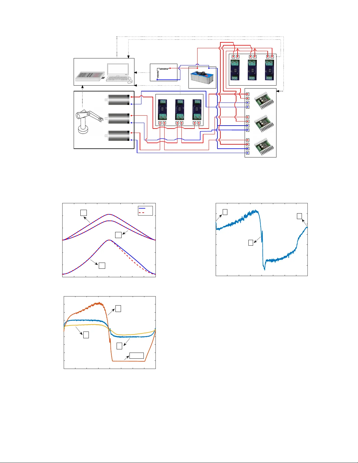
Leave a Comment