Efficient Sparse Code Multiple Access Decoder Based on Deterministic Message Passing Algorithm

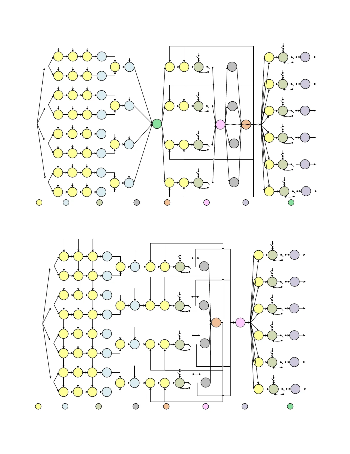
IEEE TRANSA CTIONS ON , 2018 1 Ef ficient Sparse Code Multiple Access Decoder Based on Deterministic Message P assing Algorithm Chuan Zhang, Member , IEEE , Chao Y ang, W ei Xu, Senior Member , IEEE , Shunqing Zhang, Senior Member , IEEE , Zaichen Zhang, Senior Member , IEEE , and Xiaohu Y ou, F ellow , IEEE Abstract —Being an effective non-orthogonal multiple access (NOMA) technique, sparse code multiple access (SCMA) is promising for future wireless communication. Compared with or- thogonal techniques, SCMA enjoys higher overloading tolerance and lower complexity because of its sparsity . In this paper , based on deterministic message passing algorithm (DMP A), algorithmic simplifications such as domain changing and probability ap- proximation are applied for SCMA decoding. Early termination, adaptive decoding, and initial noise reduction are also employed for faster conv ergence and better performance. Numerical results show that the proposed optimizations benefit both decoding complexity and speed. Furthermore, efficient hardware archi- tectures based on f olding and retiming are proposed. VLSI implementation is also given in this paper . Comparison with the state-of-the-art hav e shown the proposed decoder’ s advantages in both latency and throughput (multi-Gbps). Index T erms —Sparse code multiple access (SCMA), determin- istic message passing algorithm (DMP A), folding, retiming, VLSI. I . I N T RO D U C T I O N T HE fifth generation of cellular network (5G) is put forward to meet the ever -increasing demand of wire- less communication. Enabling techniques of 5G include mas- siv e multiple-input multiple-output (MIMO), adv anced coding, new multiple access (MA), full spectrum access, ne w network architectures, etc [1]. In the past decades, MAs such as time di vision multiple access (TDMA) [2], frequency division multiple access (FDMA) [3], and code di vision multiple access (CDMA) [4], became part of wireless standards. Howe ver , those orthogonal MAs can hardly meet the 5G’ s capacity requirement ( 10 3 times of L TE), due to limitations on multi- plexing approaches towards physical resources [5]. According to 3GPP white book, in the enhanced Mobile Broadband (eMBB) scenario, the peak data rate should be 20 Gbps ( 10 to 10 2 times of L TE), the peak spectral efficienc y should be 30 bps/Hz ( 3 to 5 times of L TE), and the latenc y should be less Chuan Zhang and Chao Y ang are with Lab of Efficient Architectures for Digital-communication and Signal-processing (LEADS), Southeast Uni versity , Nanjing, China. Chuan Zhang, Chao Y ang, W ei Xu, Zaichen Zhang, and Xi- aohu Y ou are with the National Mobile Communications Research Laboratory , Southeast University , Nanjing, China. Chuan Zhang, Chao Y ang, and Zaichen Zhang are with Quantum Information Center of Southeast Uni versity , Nanjing, China. Email: { chzhang, chaoyang, wxu, zczhang, xhyu } @seu.edu.cn. Shunqing Zhang is with Shanghai Institute for Advanced Communica- tions and Data Science, Shanghai Uni versity , Shanghai, China. Email: shun- qing@shu.edu.cn. This paper was presented in part at IEEE Asia Pacific Conference on Circuits and Systems (APCCAS), Jeju, Korea, 2016, as a Best Paper A ward recipient. Chuan Zhang and Chao Y ang contributed equally to this work. (Corr esponding author: Chuan Zhang.) than 1 ms ( 10% of L TE) [6, 7]. Thus, ideas of non-orthogonal MA (NOMA) [8] are proposed to alleviate these bottlenecks. A. Challenges for Existing NOMA Compared to orthogonal MAs, NOMA techniques refer to those allowing multiple users overlap in time, frequency , or code domain, in other words, sharing the same physical resources [9]. NOMA is able to distinguish dif ferent users via successi ve interference cancellation (SIC) [10] or multiple user decoding (MUD) [11]. Besides the very first version [12], the state-of-the-art (SOA) NOMA includes multiuser shared access (MUSA) [13], pattern division multiple access (PDMA) [14], sparse code multiple access (SCMA) [15], etc. SIC was employed in [12 – 14] and has practical challenges: • Computational complexity: SIC implies that each user can be decoded only when all the prior users are properly decoded. Therefore, its computational complexity scales with the in-cell user number . • Error propagation: For SIC, if an error occurs, all users afterward are likely to be decoded incorrectly . • Decoding latency: User power sorting is inv olved in SIC, and causes good ov erhead latency compared to other methods. Since the data with the lowest po wer is decoded last, the latenc y will even higher . Therefore, SCMA employs MUD instead of SIC. Thanks to its sparsity , message passing algorithm (MP A) can be applied for better decoding performance. B. Sparse Code Multiple Access SCMA was proposed in 2013 [15], trying to increase user scale via a ne w perspectiv e: enabling more efficient multiple access by non-orthogonal sparse spreading codes of users. 1) Properties of SCMA: As a promising MA, SCMA has the properties: i) multiplexing in frequency domain; ii) codebook based on both mapping and spreading; iii) multi- dimensional constellation for shaping gain and spectral effi- ciency; iv) non-orthogonality ensuring more accessed users; v) spreading which reduces noise interference and enhances system robustness; and vi) sparsity which reduces decoding complexity . Thanks to these properties, SCMA is more phys- ically realizable and overloading tolerant, compared to other MAs [16]. Details of SCMA can be found in Section II. 2) Challenges of SCMA: • Throughput: Though the throughput of SCMA outper- forms other MAs, especially orthogonal ones, it is hard to 2 IEEE TRANSA CTIONS ON , 2018 achiev e the eMBB peak rate with acceptable complexity . Admittedly , such throughput can be achiev ed with a larger overloading factor , leading to prohibitive hardware complexity and performance de gradation. • Latency: On one hand, utilizing MUD, SCMA av oids the sorting latency required by SIC. On the other hand, for imperfect channels the iterati ve MP A tends to cost more iterations, which will counteract its latency advantage. • Implementation: Though VLSI techniques ensure that complexity is no longer a bottleneck for SCMA imple- mentation when the overloading factor is not extremely large, existing iterati ve algorithms are not hardware friendly . Second, the noise power density N 0 results in large data range, leading to unbearable quantization length, or otherwise poor error performance. C. Relevant Prior Art Regarding SCMA decoding, existing literature mainly focus on three aspects: i) stochastic computing, ii) tree structure approximation, and iii) efficient hardware implementation. 1) Stochastic Computing: In [17], a stochastic MP A (SMP A) decoder was proposed, where beliefs are giv en by weights of bit streams. Multiplication and addition are im- plemented by A N D and M U X , respecti vely . Though it work effecti vely reduces the complexity per iteration, problems are: • Accuracy: Stochastic computing suffers from lo w accu- racy , due to randomness loss. Beliefs in MP A usually require precision of 10 − 5 , which length-limited could not giv e. Performance degradation is observed. • Latency: For SMP A, the calculation of a single value re- quires a large number ( 10 5 to 10 6 ) of bit-lev el operations. Considerable iterations make the latency even larger and not suitable for practice. • Complexity: Though SMP A helps to reduce hardware of a single operation, the amount of bit-operations in one decoding is around 10 7 . Thus, the total complexity may be even larger than deterministic MP A (DMP A). A VLSI architecture of SMP A was discussed in [18]. The throughput for a 6 -user decoder is 57 Mbps and far from 3GPP requirements. Though the hardware cost is low , the latency is not suitable for eMBB. 2) T r ee Structure Appr oximation: In [19], a pruned tree approximation was proposed. The decoder accurately repre- sents values with high probabilities, whereas approximates ones with lo w probabilities [20]. Squares are replaced by ad- ditions, multiplications, and comparisons. Though complexity is expected to reduce, search breadth must be larger than 2 for performance, which increases the comple xity again. 3) Efficient Har dware Ar chitectur e: In [21], a stage-le vel folded architecture for DMP A was proposed with considera- tion of both speed and efficiency , which is our prior work. Howe ver , only theoretical analysis and simple architecture were given. The real VLSI implementation is missing. D. Contributions This paper emphasises on iteration reduction, con vergence speedup, computation simplification, and implementation of SCMA decoder . Compared to SOA, our contrib utions are: • W e propose early termination scheme based on the con- ver gence beha vior of DMP A, which significantly reduces the required iteration number . • W e propose adaptiv e decoder, which adjusts beliefs ac- cording to the variation trend, accelerates the con ver- gence, and compensates the performance loss. Results show that it outperforms the ones in [17, 18] in terms of latency and throughput, satisfying the 3GPP require- ments. • W e perform numerical analysis for conditional probability approximation (over 60% computation is for conditional probabilities in MP A) in Initialization , which is square- free and division-free, and suffers from little performance loss. Computational complexity and hardware implemen- tation have been greatly benefitted. • W e propose distributed matrix scheme for prior noise reduction of DMP A decoder, which compensates the approximation loss with negligible extra complexity . • W e improve our stage-lev el folded decoder with the proposed algorithms, achiev e higher hardware efficiency with eMBB requirements on throughput and latency . • W e implement the proposed DMP A decoder on Xilinx V irtex-7 XC7VX690T FPGA to demonstrate its advan- tages for real applications. E. Notations Lowercase and uppercase boldface letters designate column vectors and matrices, respectively . Matrix A ’ s transpose and conjugate are A T and A H . The M × M identity matrix is I M and the M × N all-zeros matrix is 0 M × N . Sets are denoted by uppercase calligraphic letters A , with cardinality |A| . F . P aper Outline The remainder of this paper is organized as follows. Section II re vie ws the preliminaries of SCMA. DMP A and its opti- mized versions are discussed in Section III. Numerical results and analysis are given in Section IV. Hardware architecture is described in Section V. VLSI implementation is giv en in Section VI. Section VII concludes the entire paper . I I . P R E L I M I N A R I E S Preliminaries of SCMA are giv en in this section. A 6 -user system in Fig. 1 is used as a running example. A. SCMA Encoder Suppose codew ord set, constellation set, and information set are X , C , and B , respectively . Define x ∈ X , c ∈ C , and b ∈ B . |B | = M , |X | = K , and |C | = N . The SCMA encoding is given by two rounds of mapping [15]. The first round of mapping is: g : B → C , c = g ( b ) , (1) where B ⊂ B log 2 M , C ⊂ C N , and g is a constellation mapping function. The second round of mapping is: V : C → X , x = Vc , (2) C. ZHANG et al. : EFFICIENT SP ARSE CODE MUL TIPLE ACCESS DECODER BASED ON DETERMINISTIC MESSA GE P ASSING ALGORITHM 3 Channel Coding SCMA Encoder ĂĂ Channel Coding SCMA Encoder Channel Coding SCMA Encoder Codebook 1 00 01 10 11 Codebook 6 00 01 10 11 User 1 User 2 User 6 b1 b2 b6 Encoded bits 1 x 2 x 3 x 4 x RE1 RE2 RE3 RE4 RN RN RN RN LN LN LN LN LN Channel Decoding Channel Decoding Channel Decoding Ă Ă LN Ă User 1 User 3 User 6 Resource Node Layer Node Reciever 0 0 a * b - 0 a 0 b 0 0 * b * a - 0 0 * b - * a 0 e 0 * d 0 c d 0 0 f 0 * e 0 0 * f * e Fig. 1. A 6 -user SCMA system. where X ⊂ C K , and V ∈ B K × N is the mapping matrix. Suppose the entire mapping function of SCMA encoding is f . Then we ha ve f : B → X , x = f ( b ) , f = V g . (3) An M -size SCMA codebook consisting of K complex values is constructed. Note that V contains ( K − N ) all-zero rows. Mapping matrix is generated by inserting ( K − N ) all-zero rows into an N × N identity matrix I N randomly . So when the SCMA system is re gular , it supports C N K = C K − N K different layers (users). B. SCMA Multiple xing Consider a K -dimensional SCMA encoder with J separated layers. Each layer is defined by ( V j , g j , M j , N j ) , where j = 1 , ..., J . If i 6 = j , V i 6 = V j and g i 6 = g j , in order to distinguish one layer from another . In general, M j and N j can be either the same or different for different layers. W ithout loss of generality , for ∀ j we set M j = M , N j = N . W e call this SCMA system semi-regular because J is not necessarily C N K (The regular system will be discussed later). The SCMA code words are multiplexed over K shared orthogonal resources, e.g. OFDMA tones or MIMO spatial layers [16]. W ith this semi-regular system, the received signal after synchronous layer multiplexing can be expressed as y = Σ J j =1 diag ( h j ) x j + n , (4) where h j and x j are the K -dimensional channel vector and SCMA code word of layer j . Suppose signals of all layers are from the same transmit point, for a specific receiv er , the channel vectors of all layers are identical that for ∀ j , h j = h . Now Eq. (4) reduces to y = diag ( h )Σ J j =1 x j + n . (5) Define overloading factor as λ = J /K , which indicates the ov erloading tolerance or access ability of a SCMA system. Fig. 2 illustrates a 6 -user SCMA multiplexing. Codebook 1 Codebook 2 Codebook 3 Codebook 4 Codebook 5 Codebook 6 Fig. 2. SCMA multiplexing example. C. F actor Graph Representation Define the binary indicator vector as f j = diag ( V j V T j ) . Then the factor graph matrix is F = ( f 1 , ..., f J ) . Then the factor graph representation can be obtained like how we do with LDPC codes. Each column of F associates a layer node, and each row a resource node. Degree of each resource node is defined as d f = ( d f 1 , ..., d f K ) T = Σ J j =1 f j . For more details, please refer to [15]. T ake K = 4 and N = 2 as an example. The factor graph is in Fig. 3 and J = C 2 4 = 6 . Degree d f = ( d f 1 , ..., d f K ) T = (3 , 3 , 3 , 3 , 3 , 3) T and the o verloading factor λ = J /K = 1 . 5 . The 4 × 6 factor graph matrix of this system is in Eq. (6). 1 L 2 L 3 L 4 L 5 L 6 L 1 R 2 R 3 R 4 R Fig. 3. Factor graph representation of an SCMA with K = 4 and J = 6 . F =     1 1 1 0 0 0 1 0 0 1 1 0 0 1 0 1 0 1 0 0 1 0 1 1     (6) I I I . O P T I M I Z AT I O N S O N S C M A D E C O D I N G A. Regular F orm of SCMA Regular SCMA refers to the absolute-regular form [22, 23], where number of layers J equals to C N K . In other words, it employs all the av ailable layers (users). Eq. (6) is an example of regular form. The definition is as follows. Definition 1. SCMA with K complex-dimension and weight of N which satisfies the following requir ements is called re gular (absolute-r egular) SCMA. Requir ement 1 : Owning J = C N K layers (users) in total. Requir ement 2 : The columns of factor graph matrix must be listed in the sequential permutation or der , with weight λ . B. DMP A Decoding The DMP A decoding for SCMA mainly includes 4 steps. 4 IEEE TRANSA CTIONS ON , 2018 1) Initialization: Calculate conditional probability with ex- trinsic information to get prepared for the belief propagation. P k ( y k | x k, 1 , x k, 2 , x k, 3 , N 0 ) = e −k y k − ( x k, 1 + x k, 2 + x k, 3 ) k 2 / N 0 , (7) where y k denotes the k -th bit of the recei ved signal y . x k, 1 , x k, 2 , and x k, 3 denote ov erlapped bits of the 3 layers which are connected to the k -th resource node separately , and N 0 is the noise po wer density . 2) Resource Node Updating: The updating formulation of resource node is in the sum-product form which is an approximation of mar ginal probability: I R k → L 1 ( m 1 ) = P M m 2 =1 P M m 3 =1 P k I L 2 → R k ( m 2 ) I L 3 → R k ( m 3 ) , (8) I R k → L 2 ( m 2 ) = P M m 1 =1 P M m 3 =1 P k I L 1 → R k ( m 1 ) I L 3 → R k ( m 3 ) , (9) I R k → L 3 ( m 3 ) = P M m 1 =1 P M m 2 =1 P k I L 1 → R k ( m 1 ) I L 2 → R k ( m 2 ) , (10) where R k is the k -th resource node, m 1 , 2 , 3 = 1 , ..., M are transmitted symbols. I R k → L 1 , 2 , 3 denotes the belief propagated to the k -th resource node from the neighboring layer nodes. I L 1 , 2 , 3 → R k is the belief passing in the opposite direction. 3) Layer Node Updating: The normalization makes sure belief falls in [0 , 1] . I L j → R 1 ( m ) = nor maliz e ( I R 2 → L j ( m )) , (11) I L j → R 2 ( m ) = nor maliz e ( I R 1 → L j ( m )) , (12) where m = 1 , ..., M corresponds dif ferent symbols. 4) Probability Calculating and Symbol Judging: After it- erations, the final probability of each symbol is Q L j ( m ) = I R 1 → L j ( m ) · I R 2 → L j ( m ) . (13) where L j denotes the j -th layer . The symbol with the highest probability becomes the estimated symbol ˆ l for each layer . C. Max-Log Algorithm Decoder in probability domain suffers from huge complex- ity and relati vely high latency . Therefore, its Max-Log version is considered [24] with the Jacobi’ s logarithm formula [25]: log N X i =1 exp( f i ) ! ≈ max i =1 ,...,N { f 1 , f 2 , ..., f N } . (14) Updating steps no w become: 1) Initialization: P log k ( y k | x k, 1 , x k, 2 , x k, 3 , N 0 ) = − 1 N 0 k y k − ( x k, 1 + x k, 2 + x k, 3 ) k 2 , (15) 2) Resource Node Updating: I log R k → L 1 ( m 1 ) = max n P log k + I log L 2 → R k ( m 2 ) + I log L 3 → R k ( m 3 ) o , (16) I log R k → L 2 ( m 2 ) = max n P log k + I log L 1 → R k ( m 1 ) + I log L 3 → R k ( m 3 ) o , (17) I log R k → L 3 ( m 3 ) = max n P log k + I log L 1 → R k ( m 1 ) + I log L 2 → R k ( m 2 ) o , (18) 3) Layer Node Updating: I log L j → R 1 ( m ) = I log R 2 → L j ( m ) , (19) I log L j → R 2 ( m ) = I log R 1 → L j ( m ) , (20) 4) Probability Calculating and Symbol Judging: Q log L j ( m ) = I log R 1 → L j ( m ) + I log R 2 → L j ( m ) . (21) D. Early T ermination Early termination is based on the belief judgement for each layer node and resource node [26]. Our judgement steps are: 1) Create a zero-matrix to record the stability condition of beliefs, which denotes all the beliefs are unstable. 2) Judge the stability of all beliefs per iteration. If | V − V temp V temp | ≤ , (  > 0) , the beliefs are stable, and the corresponding value in the matrix is set as “ 1 ”. 3) When the stability matrix become a all-ones matrix, beliefs of all layer nodes and resource nodes are stable, and the con vergence is achieved. Then, the iterative decoding terminates. Here, V temp and V are the belief values in the previous and present iteration, respecti vely .  is a judgment constant. The DMP A with early termination is shown in Alg. 1. The Max- Log version is similar and omitted. Algorithm 1 DMP A with Early T ermination Input: y , I max , and  1: Iteration: 2: for t = 1 : I max 3: Set stability matrix S = 0 4: Update beliefs V 5: for j = 1 : N 6: temp =   V ( t ) j − V ( t − 1) j /V ( t − 1) j   7: if temp ≤  8: S j = 1 9: end if 10: end f or 11: if S = 1 12: break 13: end if 14: end f or 15: Judgement early : 16: Compute beliefs 17: Decide ˆ u Output: ˆ u = { ˆ u 1 , ˆ u 2 , ..., ˆ u 6 } E. Self-Adaption Algorithm Self-adaption [27, 28] is also based on stability judgement. Compared to the one in early termination, the judgement in self-adaption requires an extra step between 2) and 3): “Forecast and adjust the belief of next iteration based on the con ver gence trend. If V − V temp V temp ≥  , V ⇐ αV with α > 1 , since the con ver gence trend makes values larger . Otherwise, if V − V temp V temp ≤ −  , V ⇐ β V with β < 1 . ” Now the DMP A with self-adaption is shown in Alg. 2. The Max-Log version is omitted. C. ZHANG et al. : EFFICIENT SP ARSE CODE MUL TIPLE ACCESS DECODER BASED ON DETERMINISTIC MESSA GE P ASSING ALGORITHM 5 Algorithm 2 DMP A with Self-Adaption Input: y , I max , and  1: Iteration: 2: for t = 1 : I max 3: Set stability matrix S = 0 4: Update beliefs V 5: for j = 1 : N 6: temp = V ( t ) j − V ( t − 1) j /V ( t − 1) j 7: if temp ≥  8: V ( t ) j ← α · V ( t ) j 9: elseif temp ≤ −  10: V ( t ) j ← β · V ( t ) j 11: else 12: S j = 1 13: end if 14: end f or 15: if S = 1 16: break 17: end if 18: end f or 19: Judgement adapt : 20: Compute beliefs 21: Decide ˆ u Output: ˆ u = { ˆ u 1 , ˆ u 2 , ..., ˆ u 6 } Multiplex inverse matrix Transmitter a b c d 0.1 0.4 0.3 0.2 0.2 0.1 0.4 0.3 0.3 0.2 0.1 0.4 0.4 0.3 0.2 0.1 é ù ê ú ê ú ê ú ê ú ë û Distributed matrix D A B C D Subcarrier 1 Subcarrier 2 Subcarrier 3 Subcarrier 4 transmit A B C D Noise ( ) 2 0, s Soft decoding Wireless Channel Fig. 4. Procedure of initial noise reduction. F . Initial Noise Reduction “Distributed matrix” D is to reduce random error, enhance accuracy of initial value [29], and speed up the con vergence. For the SCMA system in Fig. 4, we hav e the ov erlapped signals: a , b , c , and d after multiplexing. Random error of these signals can be either positive or negati ve, which depends on the en vironment noise. Therefore, we can re group signals and assign them to 4 resource nodes. At the recei ver , we can first recover the original signals according to the inv erse of “distributed matrix” and then start the decoding. Compared to original transmitting scheme, each signal of specific resource node has a great chance to be added with both positive and negati ve random noises, which increases the accuracy of initial value. It is noted that D is not constant and can be adjusted according to the codebook and channel condition. G. Initial Pr obability Appr oximation Discussed abov e, the calculation of initial probability results in high computational comple xity , which is obvious in Max- Log decoding. Thus, suitable approximations in Initialization are expected to improve calculation efficiency and reduce latency with little performance loss. For SCMA decoding, the purpose of iterativ e updating is to find the symbol with the largest probability . Hence, the absolute value is not that critical to mak e a decision. W e can still ensure the detection correctness even with relati ve beliefs. The relati ve magnitude is determined by the initial probability and the initial value of different users in Initialization . Now , we carry out the approximation in steps: i) simplify the initial probability calculation by reducing operations with large comple xity; ii) adjust the initial v alue of different users according to the relati ve magnitude determined by initial probabilities; iii) update beliefs iterativ ely based on the relativ e values. The formulae of initial probabilities in DMP A become: P k ( y k | x k, 1 , x k, 2 , x k, 3 , N 0 ) = e −k y k − ( x k, 1 + x k, 2 + x k, 3 ) k 2 / N 0 , (22) For square and di vision, which are of higher complexity , DMP A approximations 1 to 3 are proposed: P k ( y k | x k, 1 , x k, 2 , x k, 3 , N 0 ) = e −k y k − ( x k, 1 + x k, 2 + x k, 3 ) k / N 0 , (23) P k ( y k | x k, 1 , x k, 2 , x k, 3 , N 0 ) = e −k y k − ( x k, 1 + x k, 2 + x k, 3 ) k 2 , (24) P k ( y k | x k, 1 , x k, 2 , x k, 3 , N 0 ) = e −k y k − ( x k, 1 + x k, 2 + x k, 3 ) k , (25) Similarly , we have Max-Log approximations 1 to 3 as follows. P log k ( y k | x k, 1 , x k, 2 , x k, 3 , N 0 ) = − 1 N 0 k y k − ( x k, 1 + x k, 2 + x k, 3 ) k , (26) P log k ( y k | x k, 1 , x k, 2 , x k, 3 , N 0 ) = − k y k − ( x k, 1 + x k, 2 + x k, 3 ) k 2 , (27) P log k ( y k | x k, 1 , x k, 2 , x k, 3 , N 0 ) = − k y k − ( x k, 1 + x k, 2 + x k, 3 ) k , (28) Analysis belo w will show these approximations hav e different effects on error performance and computational complexity . I V . R E S U LT S A N D A NA L Y S I S A. Error -Rate P erformance The 6 -user SCMA system is simulated. Additional white Gaussian noise (A WGN) is assumed. The maximum iteration number is 5 . Results are giv e in Fig. 5. Fig. 5(a) shows the BLER performance of DMP A algorithm with different approximations, different iterations, early ter- mination, self-adaption, and initial noise reduction. Fig. 5(b) shows the curves of Max-Log algorithm. According to Fig. 5, we see 1) DMP A/Max-Log with more iterations enjoys better per- formance, but the improv ement is limited when iteration number is suf ficiently large. Shown by numerical results, DMP A/Max-Log with 3 iterations is a good choice in real implementation. 2) The average iteration number of early termination or adaptiv e scheme is around 3 , but the performance is similar DMP A with 5 iterations. Results with different parameters reveal that self-adaption performs better in 6 IEEE TRANSA CTIONS ON , 2018 −2 0 2 4 6 10 −4 10 −3 10 −2 10 −1 10 0 SNR [dB] BLER DMPA Precise −2 0 2 4 6 10 −3 10 −2 10 −1 10 0 SNR [dB] DMPA Approximation 1 −2 0 2 4 6 10 −0.3 10 −0.2 10 −0.1 SNR [dB] DMPA Approximation 2 −2 0 2 4 6 10 −0.3 10 −0.2 10 −0.1 SNR [dB] DMPA Approximation 3 DMPA: Early DMPA: Adaptive DMPA: Iter1 DMPA: Iter2 DMPA: Iter3 DMPA: Iter4 DMPA: Iter5 (a) Error-rate performance of DMP A with different approximation. IEEE TRANSA CTIONS ON CIRCUITS AND SYSTEMS I, 2017 14 A 0 A 1 A 8 A 9 A 16 A 17 D B 0 B 1 A 2 4 B 8 C 0 1 , R e x D D D D D D D D D 2 , R e x 3 , R e x 1 , I m x 2 , I m x 3 , I m x 0 1 / N - 1 y A 2 A 3 A 1 0 A 1 1 A 18 A 19 D B 2 B 3 A 25 B 9 C 1 1 , R e x D D D D D D D D D 2 , R e x 3 , R e x 1 , I m x 2 , I m x 3 , I m x 0 1 / N - 2 y A 4 A 5 A 12 A 13 A 2 0 A 2 1 D B 4 B 5 A 2 6 B 1 0 C 2 1 , R e x D D D D D D D D D 2 , R e x 3 , R e x 1 , I m x 2 , I m x 3 , I m x 0 1 / N - 3 y A 6 A 7 A 14 A 15 A 2 2 A 2 3 D B 6 B 7 A 2 7 B 11 C 3 1 , R e x D D D D D D D D D 2 , R e x 3 , R e x 1 , I m x 2 , I m x 3 , I m x 0 1 / N - 4 y y F 0 B 12 M EM k P D D D D B 16 A 2 8 0 D D D G 0 B 1 3 B 17 A 29 0 D D D B 1 4 B 18 A 30 0 D D D B 1 5 B 19 A 31 0 D D D A 3 2 0 D A 33 0 D A 34 0 D A 35 0 D D 0 D 1 D 2 D 3 E 0 RN M EM L N M EM B 2 0 B 2 1 B 2 4 B 2 5 B 2 2 B 2 3 H 0 0 D H 1 0 D H 2 0 D H 3 0 D H 4 0 D H 5 0 D I 0 I 1 I 2 I 3 I 4 I 5 1 l 2 l 3 l 4 l 5 l 6 l 4D 4D 4D 4D D D D D D D D D D D D D D D D D D D D D Fig. 13. Data flo w graph (DFG) of step-le v el architecture. A0 A1 A 8 A 9 A 16 A 17 D B 0 B 1 A 2 4 B 8 C 0 1 , R e x D D D D D D D D D 2 , R e x 3 , R e x 1 , I m x 2 , I m x 3 , I m x 0 1 / N - 1 y A 2 A 3 A 1 0 A 1 1 A 18 A 19 D B 2 B 3 A 25 B 9 C 1 1 , R e x D D D D D D D D D 2 , R e x 3 , R e x 1 , I m x 2 , I m x 3 , I m x 0 1 / N - 2 y A 4 A 5 A 12 A 13 A 2 0 A 2 1 D B 4 B 5 A 26 B 1 0 C 2 1 , R e x D D D D D D D D D 2 , R e x 3 , R e x 1 , I m x 2 , I m x 3 , I m x 0 1 / N - 3 y A6 A7 A 14 A 15 A 2 2 A 2 3 D B 6 B 7 A 2 7 B 1 1 C 3 1 , R e x D D D D D D D D D 2 , R e x 3 , R e x 1 , I m x 2 , I m x 3 , I m x 0 1 / N - 4 y y B 1 2 D D D D B 16 A 28 0 D D D B 1 3 B 1 7 A 29 0 D D D B 1 4 B 1 8 A 30 0 D D D B 1 5 B 1 9 A 31 0 D D D A 32 0 D A 3 3 0 D A 3 4 0 D A 3 5 0 D D 0 D 1 D 2 D 3 B 2 0 B 2 1 B 2 4 B 2 5 B 2 2 B 2 3 H 0 0 D H 1 0 D H 2 0 D H 3 0 D H 4 0 D H 5 0 D I 0 I 1 I 2 I 3 I 4 I 5 1 l 2 l 3 l 4 l 5 l 6 l 4D 4D 4D 4D D D D D D D D D D D D D D D D D D D D D E 0 D D D D G 0 L N M E M RN M E M Fig. 14. Data flo w graph (DFG) of stage-le v el architecture. −2 0 2 4 6 10 −4 10 −3 10 −2 10 −1 10 0 SNR [dB] BLER Max−Log Precise (a) −2 0 2 4 6 10 −3 10 −2 10 −1 10 0 SNR [dB] Max−Log Approximation 1 (b) −2 0 2 4 6 10 −4 10 −3 10 −2 10 −1 10 0 SNR [dB] Max−Log Approximation 2 (c) −2 0 2 4 6 10 −3 10 −2 10 −1 10 0 SNR [dB] Max−Log Approximation 3 (d) Max−Log: Early Max−Log: Adaptive Max−Log: Iter1 Max−Log: Iter2 Max−Log: Iter3 Max−Log: Iter4 Max−Log: Iter5 (e) Fig. 15. Error -rate performance of DMP A with dif ferent approximation and detecting methods. (b) Error-rate performance of Max-Log with different approximation. Fig. 5. Error-rate performance of SCMA with different detecting methods. high SNR. Thus, the adjusting factor in self-adaption is supposed to be smaller at higher SNR. 3) DMP A and Max-Log hav e similar performance without approximation. Ho wev er , since DMP A hea vily depends on N 0 , approximations without precise N 0 will cause unbearable performance loss. On the other hand, Max- Log algorithm is not sensitive to N 0 , and its approxi- mations without exact N 0 can still achieve good perfor- mance. Therefore, Max-Log is preferred. Now , we figure out that suitable configurations for hardware implementation are: i) Max-Log approach; ii) 3 iterations; iii) early termination and self-adaption; i v) Approximation 2 or 3 , and v) initial noise reduction. B. Computational Comple xity Suppose the symbol set size for each user is M , the number of physical resources is N , the user number is K , and the maximum iteration number is I . Then, we summarize the computational complexity of different decoding methods in T able I. Compared with other methods, the proposed method has the lowest computational complexity , while maintaining the error performance. In fact, the proposed method is similar to Max-Log, but has lower complexity in Initialization due to the approximation. For a real system, M and N are usually large, the number of multiplications and di visions will makes other methods not suitable for implementation. Howe ver , as discussed above, the proposed algorithm is multiplication/division-free with Approximation 3 . Therefore, it can intensively improve the computational efficiency and reduce the latency , making it more applicable for hardware implementation in Section VI. The VLSI implementation re- sults in T able IV will further verify that the proposed decoder’ s hardware efficienc y over the SO A design. C. P erformance/Complexity T rade-Of f Analysis Fig. 6 illustrates the trade-off between error performance and computational complexity of proposed methods. The minimum required SNR to achiev e 1% BER is employed as a metric. The complexity is gi ven by Timing (TM) comple xity , which is in term of iteration number . Fig. 6 shows the trade-of f of DMP A with approximations. It is clear that Max-Log with Approximation 3 provides the best performance/complexity trade-off. 4 5 6 7 8 9 100 200 300 400 500 600 700 800 900 Minimum SNR [dB] to achieve 1% BLER Timing (TM) Complexity DMPA Precise DMPA Approx 1 Max−Log Precise Max−Log Approx 1 Max−Log Approx 2 Max−Log Approx 3 Fig. 6. Performance/complexity trade-off analysis of DMP A algorithm. V . H A R DW A R E A R C H I T E C T U R E The hardware architecture of the Max-Log DMP A is dis- cussed. T iming optimization and folding technique are intro- duced for higer efficiency . A. Overall Arc hitectur e The overall architecture is shown in Fig. 7. It has 4 units and 2 memory networks, which are RN-to-LN and LN-to-RN networks for I R → L and I L → R , respectively . The elementary units are Initialization Unit , Resource Node Update Unit , Layer Node Update Unit , and Pr obability Calculating Unit , which execute steps indicated by Eq. (15) to Eq. (21), re- spectiv ely . The iterativ e calculation is done by Resour ce Node C. ZHANG et al. : EFFICIENT SP ARSE CODE MUL TIPLE ACCESS DECODER BASED ON DETERMINISTIC MESSA GE P ASSING ALGORITHM 7 T ABLE I C O M PAR I S ON O F C O M P U TA T I O N A L C O M P L E X I T Y F O R D I FF E R E N T D E C O D I NG A L G O R I T H M S Procedure Operation This work DMP A [21] Max-Log [30] Pruned DMP A [31] [APCCAS ’17] [China Comm. Dec. ’15] [DSP ’16] Initial probability calculation ADD 2 M 3 N/T adp 3 M 3 N/T MP A 3 M 3 N/T Max-Log 3 M 3 N/T tree MUL 0 3 M 3 N/T MP A 3 M 3 N/T Max-Log 3 M 3 N/T tree EXP 0 M 3 N/T MP A 0 M 3 N/T tree Resource node updating ADD 2 · 3 M 3 N 3 M 3 N 2 · 3 M 3 N 3 M 3 N MUL 0 2 · 3 M 3 N 0 2 · 3 M 3 N MAX 3 M 3 N 0 3 M 3 N 0 Layer node updating ADD 0 2 M K 0 2 M K MUL 0 2 M K 0 2 M K SWOP 2 M K 2 M K 2 M K 2 M K Users’ symbol judgement ADD M K 0 M K 0 MUL 0 M K 0 M K MAX 0 M K 0 M K R e s our c e N ode U pda te U ni t RN - to - L N N e t w or k LN - to - R N N e two r k L a ye r N ode U pda te U nit P r oba bil it y C a l c ul a t i ng U nit O utput I nit ia l iz a ti on U ni t 0 ,, N yH ˆ l Fig. 7. Overall architecture of DMP A. Update Unit and Layer Node Update Unit , both of which could not start current propagation unless all previous data have been calculated. W e call this data updating interv al a “step”. Optimization details of this scheduling will be discussed below . B. Stage-Level Scheduling Optimization ACC STO SWOP RESET Step 1 CMP , n f Step 2 Step 3 Time init L R I ® Step 4 L R I ® ACC Stage 0 network R L I ® One interation R L I ® 0 1 / N - MUL R L I ® STO R L I ® CMP SLT Stage 1 Stage 2 Stage 3 Stage 4 Stage 5 Stage 6 Stage 7 Stage 8 Stage 9 Stage 10 2 X Operand Operator After several iterations MAG L R I ® SUM SYM MUL STO SWOP RESET CMP , n f init L R I ® L R I ® R L I ® 0 1 / N - MUL R L I ® STO 2 X MAG L R I ® ACC ( ) L Q m R L I ® CMP SLT SYM Ă Ă network R L I ® 4 parallel 6 parallel ( ) L Q m SUM Fig. 8. Stage-level scheduling. The proposed stage-level scheduling is a finer-grained op- timization over the step-level scheduling. With this stage- lev el scheduling, it is con venient to insert deep pipelines to achiev e a higher throughput [32 – 34]. Compared with step- lev el scheduling, updating of stage-le vel scheduling does not hav e to wait for the completion of data computation from the previous unit, which therefore av oids low hardware- efficienc y and long processing-latenc y . In sum, stage-lev el scheduling enjoys faster processing speed and higher hardware efficienc y than the step-lev el one. Fig. 8 sho ws the stage-level scheduling. It details each computing step to achiev e a deeper pipelined structure. C. F olding The architecture of stage-le vel DMP A turns out to be very complicated in form of data factor graph (DFG). T o achiev e an efficient architecture, folding technique is emplo yed for further optimization. Since folding operation based on fine-grained architecture is difficult to be carried out, a folding scheme based on unit is considered. Fig.s 13 and 14 in appendix shows the entire step- and stage-le vel algorithms, respecti vely . Due to the page constraint, we only take a branch of Initialization Unit , which is fully-paralleled in DFG, as an example to show proposed folding details. Folding transform of other units can be conducted in the similar fashion. The DFG of the branch in Initialization Unit is sho wn in Fig. 9. imag. 1 2 real 3 7 4 5 8 9 10 12 6 11 D D D D D D D D D D D 0 1 / N - 1,im ag . x 1,real x 2, rea l x 3, real x 2, imag . x 3,imag . x Fig. 9. Original hardware of Step 1 before folding. The folding includes 3 steps: i) construct folding sets and folding equations, ii) analysis life span, and iii) allocate registers. More details of this method are explained by [35]. 1) F olding Sets and F olding Equations: Set the folding factor to 7 , we can obtain the following folding sets:      S in = { 1 , 2 , φ, φ, φ, φ, φ } , S A = { 3 , 4 , 5 , 6 , 7 , 8 , 9 } , S M = { 10 , 11 , 12 , φ, φ, φ, φ } , (29) where S in , S A , and S M denote the folding sets for inputs, adders, and multipliers, respectively . 8 IEEE TRANSA CTIONS ON , 2018 Then, folding equations can be deriv ed based on the giv en folding sets          D F (1 → 3) = 0 , D F (3 → 4) = 7 , D F (4 → 5) = 7 , D F (2 → 7) = 3 , D F (7 → 8) = 7 , D F (8 → 9) = 7 , D F (5 → 10) = 4 , D F (10 → 6) = 8 , D F (6 → 11) = 4 , D F (9 → 12) = 2 , D F (12 → 6) = 6 , (30) where D F ( x → y ) denotes the number of delays on the path from x to y .                          Cycle Activated number                       Fig. 10. Life time figure. 2) Life T ime Analysis: Life span analysis is demonstrated in the form of life time figure as shown in Fig. 10. It is achie ved from folding equations. One thick line in the figure represents surviv al time of certain data. Activ ated number shows number of data in use at the moment [36]. According to Fig. 10, we see that this folding architecture requires at least 8 registers. 3) Register Allocation: The forward-backward scheme of register allocation is employed based on life span analysis [37]. The specific allocation process is displayed in Fig. 11. Cycle Input 1 R 2 R 3 R 4 R 5 R 6 R 7 R 8 R Output 0 1 2 n , 3 n 2 4 n , 10 n 3 n 2 n 3 5 n 3 n 2 n 4 n 10 n 4 6 n , 12 n 5 n 3 n 2 n 4 n 10 n 2 n 5 7 n 12 n 5 n 6 n 3 n 4 n 10 n 6 8 n 7 n 12 n 5 n 6 n 3 n 4 n 10 n 7 9 n 8 n 7 n 12 n 5 n 6 n 3 n 10 n 4 n 5 n 8 9 n 8 n 7 n 12 n 4 n 6 n 3 n 10 n 3 n , 6 n 9 9 n 8 n 7 n 12 n 4 n 10 n 4 n , 9 n 10 8 n 7 n 12 n 10 n 10 n , 12 n 11 8 n 7 n 12 8 n 7 n 7 n 13 8 n 8 n Fig. 11. Register allocation table of folding architecture. After all the steps, we can finally obtain the folded archi- tecture of the branch in Initialization Unit . D. Hardwar e Ar chitectur e and Loop Analysis The final stage-level folded architecture of DMP A, which is illustrated at module-lev el in Fig. 12. Lower hardware cost and reasonable processing speed become its main adv antages. The loop bound analysis [38, 39] of this folded architecture is also giv en here. Suppose the processing time of an adder , a y M E M C M P S L T ˆ l D D D D D D C M P S W O P D 2 M A G L o o p 1 L o o p 2 L o o p 3 L o o p 4 Fig. 12. Hardware architecture of DMP A. T ABLE II C O S T O F D I FF E R E N T A R C H I T E C T U R E S F O R “ J = 6 ” Different architectures Cycles Hardware cost (main untis) Adders (Comparators) Multipliers Original 80 52 12 Stage-lev el folded 300 4 2 comparator , and a swopper are T A , T C , and T S , respecti vely . W e can obtain the results listed by T able III. T ABLE III L O O P B O UN D A NA L Y S I S Loop ADD CMP SWOP Delay Loop bound 1 1 1 0 3 ( T A + T C ) / 3 2 2 1 0 4 (2 T A + T C ) / 4 3 1 1 1 4 ( T A + T C + T S ) / 4 4 2 1 1 5 (2 T A + T C + T S ) / 5 Thus, the iteration bound is calculated as follo ws: T ∞ = max  T A + T C 3 , 2 T A + T C 4 , T A + T C + T S 4 , 2 T A + T C + T S 5  (31) V I . V L S I I M P L E M E N TA T I O N The proposed decoder’ s VLSI implementation is giv en and compared to two SOA baselines. The first is the DMP A de- coder [21], and the second is the SMP A decoder [18]. As both baselines do not consider folding, the proposed decoder does not either for fair comparison. But if all designs are folded, the proposed decoder’ s adv antages remain. Discussed pre viously , the proposed decoder is based on: i) Max-Log approach; ii) early termination and self-adaption; iii) Approximation 3 , and iv) initial noise reduction. Since the SMP A decoder employed 5 iterations, 1 up to 5 iterations are considered, though 3 turns out to be efficient per our analysis. Both the proposed decoder and DMP A decoder are implemented with Xilinx V irtex-7 XC7VX690T FPGA. The results of SMP A decoder is scribed from [18], since it is implemented with ASIC. The frequency is 500 MHz. The input quantization is 8 -bit for both real and imaginary parts, and the intermediate quantization is 16 . A. Module Details of Pr oposed Decoder The proposed decoder consists of four basic parts as shown in Fig. 7: initialization module, layer node updating network, resource node updating network, and symbol judging module. The design details are presented as follows. 1) Initialization Module: It calculates initial belief of each user with the receiv ed signal and inner codebook. The receiv ed signal is made up of 4 complex resource nodes, thus the input is 8 -parallel. Each of them has the quantization length of 8 . It is noted that the output belief has the quantization length of 16 , due to multiplication. The codebook is restored in memories, which costs 96 memory blocks of 8 -bit length each. C. ZHANG et al. : EFFICIENT SP ARSE CODE MUL TIPLE ACCESS DECODER BASED ON DETERMINISTIC MESSA GE P ASSING ALGORITHM 9 2) Resource Node Updating Network: It calculates the sum of belief and outputs the largest, based on the approximated Jacobi’ s formula. It is made up of resource node updating units, where the input data are initial beliefs and layer node beliefs, and the output data are the 4 resource node beliefs. The lar gest v alue is selected from 16 intermediate beliefs, in 3 steps of comparison with 14 buf fers. Thus, 56 buf fers are required by each unit, and 672 by the entire network. 3) Layer Node Updating Network: It is made up of layer node updating units, which normalize the input value and swop it by the inner connection. In each unit, the input data are resource node beliefs only , and the output data are the corresponding 4 layer node beliefs. Four 16 -bit dividers are required per unit with 28 clocks’ delay . Hence, the whole network needs 48 dividers. Besides, layer node beliefs would also be reset at the start of each frame of the received signals in layer node updating network. 4) Symbol Judging Module: It finds the largest belief and maps it to original source code according to the codebook of each user . Also, this module consists of 6 smaller judging units, which perform the basic function for each user . In each unit, 4 beliefs are compared with each other . Thus 2 steps of comparison and 3 buf fers are required. Then, the entire module needs 18 b uffers. The implementation comparison with the DMP A decoder is listed in T able IV. It sho ws the proposed decoder’ s advantages in both complexity and throughput, thanks to the log-domain processing and approximation approaches. T ABLE IV F P G A R E S U LT S F O R D I FF E R E N T D E C O D E R S W I T H J /K = 6 / 4 SCMA decoders DMP A decoder [21] This work LUTs 139 , 205 (36%) 82 , 909 (19%) Registers 248 , 217 (28%) 109 , 997 (12%) LUT -FF pairs 103 , 127 (36%) 52 , 203 (18%) DSP48E1s 436 (12%) 436 (12%) Maximum frequency 167 . 6 MHz 359 . 1 MHz Since speed is the main focus of our design, comparison results of throughput and latency with baselines are shown in T able V, where “L ” for latency and “T” for throughput. As we can see from the table, the proposed SCMA decoder outperforms the SOA in both throughput and latency , and also meets the multi-Gbps and millisecond requirements of 3GPP . Though, SMP A decoder has complexity adv antage, the proposed decoder’ s complexity can be further reduced with folding techniques. V I I . C O N C L U S I O N In this paper , simplifications such as log-domain calculation and probability approximation have been introduced to lo wer the complexity of SCMA ’ s DMP A decoder . Early termination, adaptiv e decoding, and initial noise reduction are also pro- posed for faster con vergence and better performance. Hard- ware optimizations with folding and retiming are introduced. VLSI implementation results ha ve confirmed the adv antages of the proposed SCMA decoder for high-speed applications ov er the SOA designs. Future research will be directed towards further improvements on both algorithm and implementation. R E F E R E N C E S [1] T . B. Iliev , G. Y . Mihaylov , T . D. Bikov et al. , “L TE eNB traffic analysis and key techniques towards 5G mobile networks, ” in Pr oc. IEEE International Convention on Information and Communication T echnology , Electronics and Micr oelectr onics (MIPRO) , May 2017, pp. 497–500. [2] M. Anwar, Y . Xia, and Y . Zhan, “TDMA-based IEEE 802.15.4 for low- latency deterministic control applications, ” IEEE T rans. Ind. Informat. , vol. 12, no. 1, pp. 338–347, Feb . 2016. [3] A. N. Akansu and M. V . T aztbay , “Orthogonal trans multiplexer: A multiuser communications platform from FDMA to CDMA, ” in Pr oc. IEEE European Signal Processing Confer ence (EUSIPCO) , Sep. 1996, pp. 1–4. [4] Q. Xue, Y . Li, L. Zhong et al. , “Study on key techniques for 3G mobile learning platform based on cloud service, ” in Pr oc. IEEE International Confer ence on Consumer Electr onics, Communications and Networks (CECNet) , Apr . 2011, pp. 3588–3591. [5] J. G. Andrews, S. Buzzi, W . Choi et al. , “What will 5G be?” IEEE J. Sel. Areas Commun. , vol. 32, no. 6, pp. 1065–1082, Jun. 2014. [6] 3GPP , “Study on scenarios and requirements for next generation access technologies, ” 3r d Generation P artnership Project (3GPP) , vol. 32, no. 6, pp. 1065–1082, Mar . 2016. [7] J. Gozalvez, “T entative 3GPP timeline for 5G [mobile radio], ” IEEE V eh. T echnol. Mag. , vol. 10, no. 3, pp. 12–18, Sep. 2015. [8] W . Shin, M. V aezi, B. Lee et al. , “Non-orthogonal multiple access in multi-cell networks: Theory , performance, and practical challenges, ” IEEE Commun. Mag. , vol. 55, no. 10, pp. 176–183, Oct. 2017. [9] K. S. Ali, H. Elsawy , A. Chaaban et al. , “Non-orthogonal multiple access for large-scale 5G networks: Interference aware design, ” IEEE Access , vol. 5, pp. 21 204–21 216, May 2017. [10] Z. Dawy , A. Seeger , and M. Mecking, “Design methodologies and po wer setting strategies for WCDMA serial interference cancellation recei vers, ” in Pr oc. IEEE International Zurich Seminar on Communications (IZSC) , Oct. 2004, pp. 28–31. [11] M. A. Pasha, M. Uppal, M. H. Ahmed et al. , “T ow ards design and automation of hardware-friendly NOMA receiver with iterative multi- user detection, ” in Pr oc. IEEE ACM/ED AC/IEEE Design A utomation Confer ence (DA C) , Jun. 2017, pp. 1–6. [12] T . Manglayev , R. C. Kizilirmak, Y . H. Kho et al. , “NOMA with imperfect SIC implementation, ” in Proc. IEEE EUROCON International Confer ence on Smart T echnologies (ICST) , Jul. 2017, pp. 22–25. [13] F .-L. Luo and C. Zhang, Non-orthogonal Multi-User Superposition and Shar ed Access . W iley-IEEE Press, 2016, pp. 616–. [Online]. A vailable: http://ieeexplore.ieee.or g/xpl/articleDetails.jsp?arnumber=7572709 [14] S. Chen, B. Ren, Q. Gao et al. , “Pattern division multiple access – a novel nonorthogonal multiple access for fifth-generation radio networks, ” IEEE Tr ans. V eh. T echnol. , vol. 66, no. 4, pp. 3185–3196, Apr . 2017. [15] H. Nikopour and H. Baligh, “Sparse code multiple access, ” in pr oc. IEEE Annual International Symposium on P ersonal, Indoor , and Mobile Radio Communications (PIMRC) , Sep. 2013, pp. 332–336. [16] H. Nikopour , E. Y i, A. Bayesteh et al. , “SCMA for downlink multiple access of 5G wireless networks, ” in Proc. IEEE Global Communications Confer ence (GLOBECOM) , Dec. 2014, pp. 3940–3945. [17] K. Han, J. Hu, J. Chen et al. , “ A low complexity SCMA detector based on stochastic computation, ” in Pr oc. IEEE International Midwest Symposium on Cir cuits and Systems (MWSCAS) , Aug. 2017, pp. 783– 786. [18] ——, “ A low complexity sparse code multiple access detector based on stochastic computing, ” IEEE T rans. Cir cuits Syst. I , vol. PP , no. 99, pp. 1–14, Oct. 2017. [19] Z. Jia, Z. Hui, and L. Xing, “ A low-complexity tree search based quasi- ML recei ver for SCMA system, ” in Pr oc. IEEE International Confer ence on Computer and Communications (ICCC) , Oct. 2015, pp. 319–323. [20] M. P . C. Fossorier , M. Mihaljevic, and H. Imai, “Reduced complexity iterativ e decoding of lo w-density parity check codes based on belief propagation, ” IEEE T rans. Commun. , vol. 47, no. 5, pp. 673–680, May 1999. [21] C. Y ang, C. Zhang, S. Zhang, and X. Y ou, “Efficient hardware archi- tecture of deterministic MP A decoder for SCMA, ” in Pr oc. IEEE Asia P acific Conference on Cir cuits and Systems (APCCAS) , Oct. 2016, pp. 293–296. 10 IEEE TRANSA CTIONS ON , 2018 T ABLE V L ATE N C Y ( L ) I N [ µ S ] A N D T H RO U G HP U T ( T ) I N [ M B / S ] F O R D I FF E R E N T D E C O D E R S ( F R E Q U E N C Y : 500 M H Z ) User # ( J ) 6 12 24 48 96 192 Resource # ( K ) 4 8 16 32 64 128 Iteration # ( I max ) L / T L / T L / T L / T L / T L / T This work 1 3 . 50 / 857 . 14 3 . 70 / 1628 . 57 3 . 96 / 3012 . 85 4 . 26 / 5423 . 13 4 . 58 / 9490 . 48 4 . 95 / 16133 . 81 2 5 . 50 / 547 . 69 5 . 84 / 1040 . 62 6 . 22 / 1925 . 14 6 . 66 / 3465 . 25 7 . 16 / 6064 . 20 7 . 74 / 10309 . 14 3 8 . 62 / 349 . 96 9 . 14 / 664 . 93 9 . 74 / 1230 . 12 10 . 42 / 2208 . 46 11 . 22 / 3874 . 88 12 . 12 / 6587 . 30 4 13 . 48 / 223 . 62 14 . 28 / 424 . 88 15 . 22 / 786 . 02 16 . 32 / 1411 . 16 17 . 56 / 2475 . 96 18 . 98 / 4209 . 14 5 21 . 00 / 142 . 86 22 . 12 / 271 . 43 23 . 42 / 502 . 15 24 . 94 / 903 . 88 26 . 68 / 1581 . 78 28 . 62 / 2689 . 03 C. Y ang [21], [DMP A decoder , APCCAS ’17] 1 5 . 60 / 150 . 00 5 . 80 / 285 . 00 6 . 06 / 527 . 25 6 . 36 / 949 . 05 6 . 78 / 1660 . 84 7 . 16 / 2823 . 42 2 10 . 92 / 76 . 92 11 . 26 / 146 . 148 11 . 64 / 270 . 37 12 . 08 / 486 . 67 12 . 58 / 851 . 68 13 . 16 / 1447 . 85 3 16 . 24 / 51 . 72 16 . 76 / 98 . 27 17 . 36 / 181 . 80 18 . 04 / 327 . 23 18 . 84 / 572 . 66 19 . 74 / 973 . 52 4 21 . 56 / 38 . 96 22 . 36 / 74 . 02 23 . 30 / 136 . 94 24 . 40 / 246 . 50 25 . 64 / 431 . 37 27 . 06 / 733 . 34 5 26 . 88 / 31 . 25 28 . 00 / 59 . 38 29 . 30 / 109 . 84 30 . 82 / 197 . 72 32 . 56 / 346 . 01 34 . 50 / 588 . 21 K. Han [18], [SMP A decoder, TCAS-I Oct. ’17] 5 n.a. / 57 n.a. / n.a. n.a. / n.a. n.a. / n.a. n.a. / 640 n.a. / n.a. [22] Ryan and W illiam, A Low-Density P arity-Check Code T utorial, P art II- The Iterative Decoder , 1st ed. The University of Arizona, 2002. [23] W . Li, B. Chen, J. Lei et al. , “Low density parity check codes with quasi-cyclic structure and zigzag pattern, ” in Pr oc. IEEE International Confer ence on Signal Pr ocessing (ICSP) , Oct. 2014, pp. 1730–1734. [24] J. Chen, A. Dholakia, E. Eleftheriou et al. , “Reduced-complexity de- coding of LDPC codes, ” IEEE T rans. Commun. , vol. 53, no. 8, pp. 1288–1299, Aug. 2005. [25] P . Robertson, E. V illebrun, and P . Hoeher, “A comparison of optimal and sub-optimal MAP decoding algorithms operating in the log domain, ” in Pr oc. IEEE International Conference on Communications (ICC) , vol. 2, Jun. 1995, pp. 1009–1013 vol.2. [26] J. Chen, R. M. T anner , C. Jones et al. , “Improved min-sum decoding algorithms for irregular LDPC codes, ” in Pr oc. IEEE International Symposium on Information Theory (ISIT) , Sep. 2005, pp. 449–453. [27] X. W u, Y . Song, M. Jiang et al. , “Adaptiv e-normalized/offset min-sum algorithm, ” IEEE Commun. Lett. , vol. 14, no. 7, pp. 667–669, Jul. 2010. [28] V . Savin, “Self-corrected min-sum decoding of LDPC codes, ” in Pr oc. IEEE International Symposium on Information Theory (ISIT) , Jul. 2008, pp. 146–150. [29] G. D. Forney and G. Ungerboeck, “Modulation and coding for linear Gaussian channels, ” IEEE Tr ans. Inf. Theory , vol. 44, no. 6, pp. 2384– 2415, Oct. 1998. [30] L. Lu, Y . Chen, W . Guo et al. , “Prototype for 5G new air interface tech- nology SCMA and performance ev aluation, ” China Communications , vol. 12, no. Supplement, pp. 38–48, Dec. 2015. [31] J. Chen, K. Han, J. Hu et al. , “Low complexity sparse code multiple access decoder based on tree pruned method, ” in Proc. IEEE Interna- tional Conference on Digital Signal Processing (DSP) , Oct. 2016, pp. 341–345. [32] S. Simon, E. Bernard, M. Sauer et al. , “A new retiming algorithm for circuit design, ” in Proc. IEEE International Symposium on Circuits and Systems (ISCAS) , vol. 4, May 1994, pp. 35–38 vol.4. [33] J. Monteiro, S. Dev adas, and A. Ghosh, “Retiming sequential circuits for low po wer, ” in Proc. IEEE International Conference on Computer Aided Design (ICCAD) , Nov . 1993, pp. 398–402. [34] K. K. Parhi, C. Y . W ang, and A. P . Brown, “Synthesis of control circuits in folded pipelined DSP architectures, ” IEEE J. Solid-State Circuits , vol. 27, no. 1, pp. 29–43, Jan. 1992. [35] Parhi and K. K, VLSI digital signal processing systems: design and implementation , 1st ed. John Wile y & Sons, 1999. [36] K. K. Parhi, “Calculation of minimum number of registers in arbitrary life time chart, ” IEEE T rans. Cir cuits Syst. II , vol. 41, no. 6, pp. 434– 436, Jun. 1994. [37] ——, “Systematic synthesis of DSP data format conv erters using life- time analysis and forw ard-backward register allocation, ” IEEE Tr ans. Cir cuits Syst. II , v ol. 39, no. 7, pp. 423–440, Jul. 1992. [38] D. Y . Chao and D. T . W ang, “Iteration bounds of single-rate data flow graphs for concurrent processing, ” IEEE T rans. Circuits Syst. I , vol. 40, no. 9, pp. 629–634, Sep. 1993. [39] K. Ito and K. K. Parhi, “Determining the iteration bounds of single-rate and multi-rate data-flow graphs, ” in Proc. IEEE Asia-P acific Conference on Circuits and Systems (APCCAS) , Dec. 1994, pp. 163–168. C. ZHANG et al. : EFFICIENT SP ARSE CODE MUL TIPLE ACCESS DECODER BASED ON DETERMINISTIC MESSA GE P ASSING ALGORITHM 11 A Adder B Multiplier C Comparator D Swopper E LN Mem ory F RN M emory G Symbol Selector H P k Memory A0 A1 A8 A9 A16 A17 D B0 B1 A24 B8 1 , Re x D D D D D D D D D 2 , Re x 3, Re x 1 , Im x 2 , Im x 3, Im x 0 1 / N - 1 y A2 A3 A10 A11 A18 A19 D B2 B3 A25 B9 1 , Re x D D D D D D D D D 2 , Re x 3, Re x 1 , Im x 2 , Im x 3, Im x 0 1 / N - 2 y A4 A5 A12 A13 A20 A21 D B4 B5 A26 B10 1 , Re x D D D D D D D D D 2 , Re x 3, Re x 1 , Im x 2 , Im x 3, Im x 0 1 / N - 3 y A6 A7 A14 A15 A22 A23 D B6 B7 A27 B11 1 , Re x D D D D D D D D D 2 , Re x 3, Re x 1 , Im x 2 , Im x 3, Im x 0 1 / N - 4 y y H0 A28 MEM k P D D D D A32 C0 0 D D D F0 A29 A33 C1 0 D D D A30 A34 C2 0 D D D A31 A35 C3 0 D D D D0 D1 D2 D3 E0 RN MEM LN MEM A36 A37 A40 A41 A38 A39 C4 0 D C5 0 D C6 0 D C7 0 D C8 0 D C9 0 D G0 G1 G2 G3 G4 G5 1 l 2 l 3 l 4 l 5 l 6 l D D D D D D D D D D D D D D D D D D D D Fig. 13. Data flow graph (DFG) of step-lev el architecture. A Adder B Multiplier C Com parator D Sw opper E LN Memory F RN Memory G Symbol Selector H P k Memory A0 A1 A8 A9 A16 A17 D B0 B1 A24 B8 1 , Re x D D D D D D D D D 2 , Re x 3, Re x 1 , Im x 2 , Im x 3, Im x 0 1 / N - 1 y A2 A3 A10 A11 A18 A19 D B2 B3 A25 B9 1 , Re x D D D D D D D D D 2 , Re x 3, Re x 1 , Im x 2 , Im x 3, Im x 0 1 / N - 2 y A4 A5 A12 A13 A20 A21 D B4 B5 A26 B10 1 , Re x D D D D D D D D D 2 , Re x 3, Re x 1 , Im x 2 , Im x 3, Im x 0 1 / N - 3 y A6 A7 A14 A15 A22 A23 D B6 B7 A27 B11 1 , Re x D D D D D D D D D 2 , Re x 3, Re x 1 , Im x 2 , Im x 3, Im x 0 1 / N - 4 y y A28 A32 D D A29 A33 D D A30 A34 D D A31 A35 D D D0 D1 D2 D3 A36 A37 A40 A41 A38 A39 C4 0 D C5 0 D C6 0 D C7 0 D C8 0 D C9 0 D G0 G1 G2 G3 G4 G5 1 l 2 l 3 l 4 l 5 l 6 l D D D D D D D D D D D D D D D D D D D D E0 D D D D F0 LN MEM RN MEM C0 0 D C1 0 D C2 0 D C3 0 D Fig. 14. Data flow graph (DFG) of stage-lev el architecture.