Cracking the cocktail party problem by multi-beam deep attractor network
While recent progresses in neural network approaches to single-channel speech separation, or more generally the cocktail party problem, achieved significant improvement, their performance for complex mixtures is still not satisfactory. In this work, …
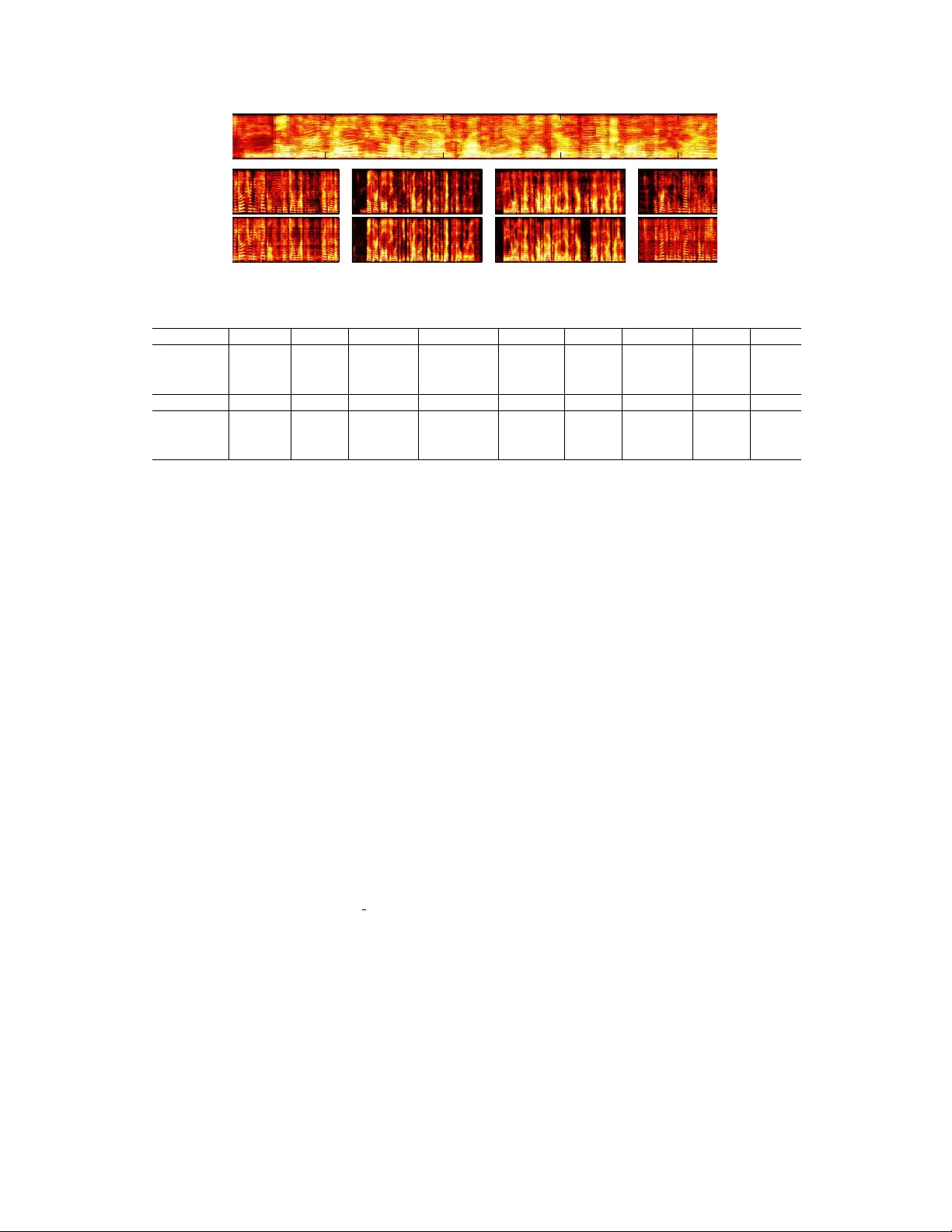
Authors: Zhuo Chen, Jinyu Li, Xiong Xiao
CRA CKING THE COCKT AIL P AR TY PR OBLEM BY MUL TI-BEAM DEEP A TTRA CT OR NETWORK Zhuo Chen, Jinyu Li, Xiong Xiao, T akuya Y oshioka, Huaming W ang, Zhenghao W ang , Y ifan Gong Microsoft AI and Research ABSTRA CT While recent progresses in neural network approaches to single- channel speech separation, or more generally the cocktail party prob- lem, achie ved significant improv ement, their performance for com- plex mixtures is still not satisfactory . In this work, we propose a nov el multi-channel framework for multi-talker separation. In the proposed model, an input multi-channel mixture signal is firstly con- verted to a set of beamformed signals using fix ed beam patterns. For this beamforming, we propose to use differential beamformers as they are more suitable for speech separation. Then each beamformed signal is fed into a single-channel anchored deep attractor network to generate separated signals. And the final separation is acquired by post selecting the separating output for each beams. T o evaluate the proposed system, we create a challenging dataset comprising mix- tures of 2, 3 or 4 speak ers. Our results show that the proposed system largely improves the state of the art in speech separation, achie ving 11.5 dB, 11.76 dB and 11.02 dB average signal-to-distortion ratio improv ement for 4, 3 and 2 overlapped speaker mixtures, which is comparable to the performance of a minimum variance distortionless response beamformer that uses oracle location, source, and noise information. W e also run speech recognition with a clean trained acoustic model on the separated speech, achie ving relati ve w ord er- ror rate (WER) reduction of 45.76%, 59.40% and 62.80% on fully ov erlapped speech of 4, 3 and 2 speakers, respectively . W ith a far talk acoustic model, the WER is further reduced. Index T erms — Cocktail party problem, Deep attractor netw ork, Differential beamforming, Neural netw ork, Speech separation 1. INTR ODUCTION The cocktail party problem has been one of the most dif ficult chal- lenges in audio signal processing for more than 60 years [1, 2, 3]. In this problem, the task is to separate and recognize each speaker in highly overlapped speech recordings, as frequently happens in a cocktail party . Although humans can solve this problem naturally without much effort, it is extremely difficult to b uild an effecti ve sys- tem to model this process. Because of the large variation in mixing sources, the cocktail party problem remains unsolved. Prior to the deep learning era [4, 5, 6, 7, 8, 9], sev eral attempts were made. The approaches proposed can be divided into two cat- egories: single-channel systems and multi-channel systems, where the difference lies in the number of recording microphones in volved. In single-channel systems, the separation process entirely relies on the spectral properties of speech, such as pitch continuity , harmonic structures, common onsets etc., and this can be achieved by using statistical models [10], rule-based models [3, 11], or decomposition- based models [12, 13, 14, 15]. In multi-channel systems, the separa- tion process can e xploit the spatial properties of each source. V ari- ous beamforming, or more precisely spatial filtering, methods were proposed by using, for example, Independent Component Analy- sis [16, 17]. Alternativ ely , clustering-based algorithms attempt to cluster time-frequency bins to individual sources by using spatial features [18, 19, 20]. There is also a clustering-based approach that uses both spatial and spectral features [21]. Howe ver , regardless of the number of microphones being used, most e xisting systems work only for rather simple scenarios, e.g. fixed speakers, limited v ocab u- lary , mixtures of dif ferent genders etc., and cannot generate satisfy- ing performance for general cases. The booming of deep learning has brought progresses in this problem. Different from most other deep learning tasks, multi-talker separation has two unique problems: a permutation problem and an output dimension problem[22, 23]. The permutation problem arises due to the fact that most deep learning algorithms require estima- tion targets to be fixed, while in multi-talker separation, arbitrary permutations of the separated sources are equiv alent. The output dimension problem refers the fact that the number of mixing speak- ers varies in different samples, which creates difficulty in learning because a neural network typically requires a fixed dimensionality at its output layer . Three single-channel neural netw ork models were proposed, namely the deep clustering(DC)[22], deep attractor network(D AN)[23] and permutation inv ariant training(PIT)[24]. In DC and D AN, each time-frequency bin in mixture spectrogram is mapped into a higher dimension representation, i.e. embedding, where the bins from the same speaker are closely located to each other . The two problems are solved by the affinity learning in DC and DAN. PIT was firstly proposed in [22], and was shown to achiev e comparable separation performance in [24]. PIT follows the mask learning framew ork[25, 26], where the network first generates the output mask for each target speaker , followed by an exhausti ve search of combination between the output and the clean reference to fix the permutation problem. The three algorithms largely boost the state of the art in speech separation. The e valuation showed the y achiev ed similar performance for two speaker and three speaker separation on common data sets. Although the deep learning based methods achiev ed break- through in the cocktail party problem, it is still difficult to apply them to real world applications because of two reasons. Firstly , their separation power has inherent limitation. For example, when there are 4 speakers, even for the most tractable scenario, i.e. two males and two females, single-channel separation seems almost impossible because the mixture is so complex that each speaker’ s voice is mostly masked by other speakers. Secondly , the current single-channel systems are usually vulnerable to re verberation. This would be because the re verberation blurs speech spectral cues which the single-channel separation systems leverage on to isolate each speaker . T o get rid of the current performance limitation, combining the single-channel and multi-channel approaches would be a natural di- rection to pursue, since the two approaches use dif ferent information for separation and therefore complementary to each other . Sev eral neural network based models hav e been proposed for multi-channel speech processing, such as acoustic modeling and speech enhance- ment [27, 28, 29, 30]. Howe ver , none of the existing systems is able to handle the multi-speaker scenario. For example, in [29, 30], a pre-learnt mask is required for each channel, which is impossible for this case simply because there is no e xisting system to get the mask. In [27], several pooling steps are required, which is not suitable for multi-talker scenario. T o the best of our knowledge, currently there is no system that can handle the complex multi-talker speech sepa- ration problem. In this work, we propose a novel, effecti ve yet simple multi- channel speech separation and recognition system. The system consists of a multi-channel part as well as a single-channel part. The multi-channel processing is handled by dif ferential beamformers with 12 fixed beams, equally sampled in space, and followed by the single-channel processing, implemented with anchored deep attrac- tor network[31], where a ratio mask is learned for each participating source. By combining the multi- and single-channel processing, the proposed system can fully utilize the spatial and spectral informa- tion, and overcome the obstacle inside most multi-channel systems when speakers’ location are close, thus leading to better perfor- mance than both single- and multi-channel systems. The proposed system utilizes the beam as the neural network input, it removes the complex domain processing for neural network, and decouple the spatial and spectral processing, which enables the system to be microphone geometry independent. And because of the attractor network architecture, the proposed system performs an end-to-end optimization process, and can be e xtended to an arbitrary number of sources without the permutation and the output dimension problem. The rest of the paper is organized as follows. In section 2 the proposed system is introduced. Section 3 describes the experiment setup and the results are discussed in section 4. Finally the conclu- sion is drawn in section 5 2. PR OPOSED SYSTEM A schematic diagram of the proposed system is shown in Fig. 1. The proposed system consists of a differential beamformer , which is responsible for multi-channel processing, and a single-channel anchored attractor network, which processes each outputting beam from the beamformer , further separating the beamformed audio. The motiv ation of this architecture is straightforward as follows. The single-channel system has inherent limitation in separating complex speaker mixtures. By using beamforming first, the spatial informa- tion is utilized to pre-enhance the signal, which reduces the separa- tion complexity , and can be handled by the single-channel system. The multi- and single-channel modules are introduced in Sec. 2.1 and Sec. 2.2. 2.1. Fixed beamformers The multi-channel processing part takes multi-channel microphone signals as input and provides the subsequent speech separation net- work with a set of beamformed signals. The beamformer is designed such that each beam has a different look direction. More specifically , we uniformly ’ sample’ the space of direction of arri val with a fix ed set of beamformers. Since this is feasible for any microphone arrays, we would expect to obtain a system that is not very sensitive to the geometry of the microphone array to be used. W e propose to utilize differential beamforming to define the beamformer set. Dif ferential beamformers are more attractiv e in speech separation than additiv e approaches such as delay-and-sum beamformers. Because differential beaformers can explicitly form acoustic nulls, they can better suppress interfering speakers than the additiv e beamformers when these speakers are sufficiently spatially isolated from the target speak er direction [32, 33]. In the experiments reported in Section 3, we employed a se ven- element microphone array . Six microphones were arranged in circle, at the center of which one microphone was placed. Each of the six microphones were separated by 60 degrees. The distance between the center microphone and the other microphones is 42.5 mm. The beamformer is designed follo wing [34]. In our experiments, we sim- ply used a set of 12 second-order differential beamformers to cover 360 ◦ degrees. Thus, each acoustic beam was targeted at 0 ◦ , 30 ◦ , and so on. W e empirically designed the directivity patterns for the 12 beams. In principle, there is a trade-off regarding the number of beams to use. The more beams we ha ve, the more likely one of them is to be targeted at a speaker direction. But, this may complicate the post selection task (see Section 2.3). 2.2. Anchored deep attractor network The single-channel processing of the proposed system is handled by an anchored deep attractor network (AD AN) proposed in [31], which is a variation of deep attractor netw ork (D AN) . Similar to their predecessor deep clustering, an embedding space is formed by neural network in both D AN and AD AN. The separat- ing process in D AN is straightforward: in embedding space, a repre- sentativ e vector for each source, e.g. the average embedding vector , is firstly calculated, which is defined as an attractor point, and serv es as the reference for each source. Then the similarity between the embedding vector and the attractors are calculated for each time- frequency point. This similarity reflects the “de gree of typicalness” of each time-frequency point, with respect to each source. For ex- ample, when an embedding point is close to one attractor , it means the corresponding time-frequency point is more likely to belong to the source represented by that attractor . The idea of DAN is to cal- culate a ratio mask for source separation based on the similarity be- tween the embeddings and the attractors, and the training objective function is to minimize the difference between the masked mixture speech and clean reference. Compared with DC, DAN allows for end-to-end optimization, where the separation is directly optimized, and thus lead to better performance [23]. The main difference between DAN and AD AN lies in the attrac- tor forming step. In both D AN and AD AN, the attractor is formed as a weighted average of the embedding vectors for each source. In D AN, this weight is provided by an oracle binary mask during train- ing. During testing, when the binary mask is not available, D AN adopts a K-means strategy on embedding points to approximate the oracle weights. The problem of this strategy is that a v arying degree of mismatch is often observed between training and testing condi- tions. T o fix this problem, in AD AN, the oracle mask is not used during training. Instead, an one step K-means with pre-tarined ini- tialization is used in both training and testing. In detail, the single- channel separation is carried in four steps, as shown in section 2.2.1 2.2.1. Anchor ed deep attractor network Firstly , as with DC and DAN, an embedding matrix V ∈ R T × F,K is generated by projecting the T -F bins to a high dimensional em- bedding space by the neural network, as shown in Eqn. (1), where T , F, K denotes the time, frequency and embedding axes and Φ( · ) refers to the neural network transformation. V tf ,k = Φ( X t,f ) (1) Secondly , a pre-segmentation is applied by calculating the distance of the embedding with several pre-trained points in the embedding space, which we refer to as the anchor points. More specifically , Fig. 1 . Proposed system. when there are C mixing sources, we hav e N anchors denoted as H ∈ R N × K . Each source is targeted to bind with one anchor . Then there are P = N C total number of source-anchor combinations. For each combination in P , we calculate the soft pre-segmentation W p,c,f t by normalizing the distance between each embedding point to each selected anchors, as shown in Eqn. (2). Based on the soft pre-segmentation W p,c,tf , for each combination in P , the attrac- tor A p,c,k is then calculated as the weighted average of embedding points, as shown in eqn. (3). W p,c,tf = softmax X k H p,c,k × V tf ,k ! (2) where softmax ( · ) is the softmax activ ation function over c axis. A p,c,k = P tf V k,tf × W p,c,tf P f ,t W p,c,tf (3) After the second step, we obtain P sets of attractors, one in which is used for further processing. In the third step, we compute the in-set similarity defined in Eqn. (4) for each attractor set. The in-set similarity measures the maximum similarity of any of the tw o attractors within the attractor set. Because the attractors serve as the center for each source to be separated, we select the attractor set that has the minimum in-set similarity . S p = max ( X k A p,i,k × A p,j,k ) , 1 ≤ i < j ≤ C (4) ˆ A = arg min { S p } , 1 ≤ p ≤ P (5) In the last step, as with DAN, a mask is formed for each source based on the picked attractor , as shown in Eqn. (6). The masked speech X f ,t × M f ,t,c is compared with the clean references S f ,t,c under an squared error measurement in (7). Unlike the original D AN, the oracle binary mask is not used during the training, there- fore the source information is not av ailable at training stage, lead- ing to the permutation problem. W e use permutation inv ariant train- ing [24] to fix this problem, where the best permutation of the C sources is exhausti vely searched. This is done by computing the squared error for each permutation of the masked speech outputs and selecting the minimum error as the error to generate the gradient for back propagation. M f ,t,c = softmax ( X k A c,k × V tf ,k ) (6) L = X f ,t,c k S f ,t,c − X f ,t × M f ,t,c k 2 2 (7) 2.2.2. Applying AD AN to beamformer outputs In the single-channel system, where only one input mixture is a vail- able, all the sources are required to be recov ered from the mixture in one shot. In contrast, in the proposed multi-beam architecture, mul- tiple beams are a va ilable as the input, which gi ves the single-channel processing more flexibility in measuring the objecti ve thanks to the spatial selectivity of the multi-channel processing. For example, when speakers are adequately separated in space, it is likely each speaker would dominate an individual beam. In this case, the single- channel processing only needs to pick the strongest speaker in each beam and the best separation is guaranteed to e xist in the results. If this is the case, the attractor network would reduce to a simple mask learning network. Howe ver , this assumption is unrealistic. When speakers are close to each other spatially or when there is speakers who are qui- eter than the others, certain speakers will not be the largest source in any beams. For example, more than 70% of 4-speaker mixtures in the dataset generated in Section 3 have such weaker speakers. In our single channel processing, for each beam we target 1 < G ≤ C most salient speak ers, and add an additional source for the residual signals. More specifically , for each beam, E = G + 1 output masks are firstly generated from the embedding, among which G sources are selected to compare with the clean references. This process is repeated for all the G E possibilities. Similarly to the original AD AN, PIT is used where the choice of permutation that leads to the minimum squared error error is selected and that error is used as the final error for back propagation. In actual processing, when the number of mixing speakers is more than 2, we set G = 2 and E = 3 , i.e. pick two speakers in each beam and set the rest speakers as one source. Under this strategy , the assumption is that each speaker appears in the first two strongest sources in at least one of the 12 calculated beams. W e think that this assumption is not restrictive and would be satisfied in many realistic scenarios if each acoustic beam has a nice directivity pattern. 2.3. Post selection After performing the single-channel processing for each beamformer output, E outputs will be generated for each of the B beams, result- ing in a total of E × B outputs being produced. Among them, C outputs need to be selected, each corresponding to one of the C tar- get speakers, as the final output. The outputs from the single-channel processing can be assumed to be separated to a certain degree, which simplifies the selection. Sev eral clues may be exploited to accomplish this. For example, we could rely on the assumption that the strongest speak er in one beam is more likely to be dominant in the neighboring beams. Moreover , in actual applications, speaker locations may also be detected from non-ov erlapping speech segments, which could also help to deter- mine the signals to output. Further in vestigation is needed for post selection and will be discussed in our follow-up w ork. In this paper, we used the following simple method. W e firstly calculate an affinity matrix between each of the E × B magnitude spectrogram by their Pearson correlation. W e then use spectral clustering to group the columns of the affinity matrix into C + 1 clusters. The moti v ation for using one additional cluster is to reduce the impacts of failure separation in certain beams and artifacts by isolating them in the additional cluster . In our experiments, we observed that after this step, for 92.5%, 96% and 99.5% of 4-speaker , 3-speaker and 2speaker mixtures, each mixing speaker was correctly segre gated into different clusters. Therefore, the remaining task after this spectral clustering step is just to select the output in each cluster that has the best speech quality . V arious algorithms can be used for the selection. In this work, we simply use a mean to standard variation criterion G = mean std of the wavfile to select the best result in each cluster . The determination of noisy cluster is also based on the speech quality . In this paper , we also report the performance of an oracle selection approach, where we select C outputs that have the best performances in reference to each clean signal. W e belie ve that using a more advanced speech quality estimator would achie ve separation performance comparable to that of the oracle selection. 2.4. Qualitative discussion on the proposed architecture Compared with pre vious studies in this field, we think the proposed framew ork has two main adv antages. Firstly , compared with existing systems that perform only one of either single or multi channel processing, the proposed system ex- ploits both spatial and spectral clues for separation, which has more potential in improving the performance in complex mixing condi- tions and rev erberation. Secondly , compared with adapti ve beamforming, the fixed multi-beam strategy used in the proposed framework would bet- ter serve the cocktail party problem because of two reasons. Firstly , in highly complicated mixing scenarios as in the case where there are 4 overlapping speakers, it is not possible with the current tech- nology to obtain parameters required for adaptive beamformering such as steering vectors and noise co-variance matrices. Without accurate estimates of these parameter values, the adaptive beam- former is not able to achiev e a reasonable degree of separation. When the adaptive beamformer was used as the multi-channel part of the proposed system, the poor performance in beamforming is propagated to the following single-channel step, possibly leading to further performance degradation. The multi-beam architecture is ensured to generate reasonable separation in certain beams, which will guarantee to hav e further separation in the single-channel step, i.e. their combination is always beneficial to each other . Secondly , the multi-beam architecture decouples the spatial and spectral pro- cessing. When changing the array , as long as we ensure that some of the beams do improv e the separation of the speakers, which is generally true unless all speakers are in the same beam, we are guar - anteed to get improv ed performance in the second stage. Adapti ve beamformers may produce unstable inputs and not suitable to be used as a preprocessor to the neural networks for single-channel speech separation. 3. EXPERIMENT SETUP 3.1. Data and pre-pr ocessing W e created a ne w speech mixture corpus by using utterances taken from the W all Street Journal (WSJ0) corpus because e xisting speech separation challenge data sets are not necessarily suitable for ev al- uation of our model. Three mixing conditions were considered: 2- speaker , 3-speaker , and 4-speaker mixtures. For each condition, a 10-hour training set, a 1-hour validation set, and a 1-hour testing set were created. Similarly to the setting in [23], both our training and validation sets were sampled from the WSJ0 training set si_tr_s . Thus, we call the validation set the closed set. Note, howe ver , that there was no utterance appearing in both the training and validation data. The testing data (or the open set) were generated similarly by using utterances of 16 speakers from the WSJ0 de velopment set si_dt_05 and the e v aluation set si_et_05 . The testing set had no speaker ov erlap with the training and validation sets. In each mix- ture, the first speaker was used as reference, and a mixing SNR was randomly determined for each remaining speaker in the range from -2.5 dB to 2.5 dB. For each mixture, the source signals were trun- cated to the length of the shortest one to ensure that the mixtures were fully ov erlapped. Each multi-channel mixture signal was generated as follows, where we used the image method [35] to add reverberation ef fects. Firstly , single-channel clean sources were sampled from the origi- nal corpus. Then a room with a random size was selected, where a length and a width were sampled from [1m, 10m], a height was sam- pled from [2.5m, 4m]. An absorption coef ficient was also randomly selected from the range of [0.2 0.5]. Positions for a microphone ar- ray and each speaker were also randomly determined. For each mix- ture, we ensured only up to 2 speaker to present within 30 ◦ . Then, a multi-channel room impulse response (RIR) was generated with the image method, which was con volved with the clean sources to gen- erate re verberated source signals. They were mixed with randomly chosen SNRs to produce the final mixtue signal to use. For speech recognition experiments, we created another testing set by using utterances from WSJ si_et_05 . Here, we used the utterances without pronounced punctuation. Unlike the testing data for speech separation experiments, the source signals were aligned to the longest one by zero padding. This is because signal truncation can be harmful to speech recognition. All data were downsampled to 8K Hz. The log spectral magnitude was used as the input feature for a single-channel source separation (i.e., AD AN) network, which was computed by using short-time Fourier transform (STFT) with a 32 ms Hann window shifted by 8 ms. 3.2. Neural network training The network used in our experiments consisted of 4 bi-directional long short term memory (BLSTM) layers, each with 300 forward and 300 backward cells. A linear layer with T anh activ ation func- tion was added on top of the BLSTM layers to generate embeddings for indi vidual T -F bins. In the network, 6 anchor points were used, and the embedding space had 20 dimensions. The network was ini- tialized with a single-channel trained 3 speaker separation network which we created in [31] and then finetuned on beamformed signals. T o reduce the training process complexity , for each speaker in each mixture, only the beam where the speaker had the largest SNR was used for training. For the ASR experiment, we first trained a clean acoustic model which is a 4-layer LSTM-RNN [36] with 5976 senones and trained to minimize a frame-level cross-entropy criterion. LSTM-RNNs 1 2 3 4 1 2 3 4 1 2 3 4 1 2 3 Time(s) 1 2 3 4 Fig. 2 . An example of the mixture spectrogram and the recovered speakers. The example used has similar SDR improvement as the the av erage performance among all test data.. Upper: original mixture. Middle: recovered utterance. Bottom: the clean reference. CLOSED original MBBF MBD AN OMBD AN MBIRM OGEV OMVDR IRM D AN 2 speakers -0.25 +7.28 +8.95 +11.02 +15.04 +1.82 +11.99 +10.91 +7.32 3 speakers -3.2 +6.86 +10.20 +11.76 +14.8 +4.64 +12.4 +11.74 +5.11 4 speakers -4.87 +6.24 +9.57 +11.55 +13.05 +6.23 +11.73 +12.17 +4.21 OPEN original MBBF MBDAN OMBD AN MBIRM OGEV OMVDR IRM DAN 2 speakers -0.29 +7.13 +8.84 +10.98 +12.05 +2.17 +12.00 +11.05 +7.82 3 speakers -3.24 +7.12 +9.94 +11.54 +15.9 +4.96 +12.56 +11.52 +5.16 4 speakers -4.89 +6.37 +9.53 +11.19 +12.75 +6.24 +11.82 +12.22 +4.23 T able 1 . The SDR(dB) improvement for 2,3 and 4 speaker mixture in closed and open speak er set hav e been shown to be superior than the feed-forward DNNs [36], which we previously verified with Microsoft Cortana task [37]. Each LSTM layer has 1024 hidden units and the output size of each LSTM layer is reduced to 512 using a linear projection layer . There is no frame stacking, and the output HMM state label is delayed by 5 frames as in [36], with both the singular v alue decomposition [38] and frame skipping [37] strategies to reduce the runtime cost. The in- put feature is the 22-dimension log-filter-bank feature e xtracted from the 8k sampled speech wa veform [39]. The transcribed data used to train this acoustic model comes from 3400 hours of US-English Cor- tana audio. W e also built a far -talk ASR model with the domain adaptation method [40] based on teacher-student (T/S) learning [41]. In [40], it was shown this T/S learning method is very effecti ve in produc- ing accurate target-domain model. The far-talk data is simulated from the 3400 hours clean data by using the room impulse response collected from public and Microsoft internal databases. The clean data is processed by the clean model (teacher) to generate the cor- responding posterior probabilities or soft labels. These posterior probabilities are used in lieu of the usual hard labels deriv ed from the transcriptions to train the tar get far -talk (student) model with the simulated far -talk data. 3.3. Evaluation Signal-to-distortion ratio (SDR), calculated by bss eval tool box[42], was used to measure the output speech quality . W e report av erage SDR improvement as well as SDR improv ement for top speakers, i.e. the speak ers who have larger mixing SNRs. The ASR performance was e v aluated in terms of word error rate (WER). T o better evaluate the proposed system, six baseline systems were included in our ev aluation. W e firstly include three oracle beamforming systems: the multi-beam beamformer(MBBF), the or- acle generalized eigen v alue (OGEV) beamformer [29] and the ora- cle minimum variance distortionless response (OMVDR) [43] beam- former . W e used the implementation of [29] for OGEV and that of [30] for OMVDR. In OGEV , for each speaker , oracle target and noise covariance matrices were calculated from the clean target and the mixture of the rest speakers. In OMVDR, for each speaker , a steering vector was calculated with the known speaker and micro- phone locations, and oracle noise covariance matrices were calcu- lated from the mixture of the rest speakers. W e also tried the oracle MVDR that used only tar get speak er directions, which is more prac- tical. Howe ver , the performance was significantly worse than all other systems, and therefore we do not report its result. In MBBF , the oracle beam selection strategy was adopted. That is, for each speaker , we picked the beam that had largest SDR for that speaker . It should be note that after the MBBF step, most of the beams are still highly mixed because the spatial separation capability of fixed beamformers is limited. Therefore the post selection method de- scribed in Sec. 2.3 did not work here. W e also included the single and multi-channel ideal-ratio-mask (IRM) system for comparison, where a mixture spectrogram was masked by oracle IRMs [44] for each target speaker, and con verted to a time domain signal with noisy phase information. As regards the multi-chanel IRM (MBIRM), the multi-channel mixture signal was first processed by the differential beamformer . Then, for each speaker , the IRM approach was applied to the beamformed signal that had the largest SDR for that speaker . Finally , we also included the single-channel anchored deep attractor network as the baseline, which was trained on the channel 0 of our multi-channel training data. 4. EXPERIMENT RESUL TS All results are reported in T ables 1–3. Figure 2 shows one separa- tion example, which has a similar SDR gain to the the average SDR improv ement ov er the whole test data. 4.1. Speech separation In T able 1, MBDAN refers to the proposed system with spectral clustering-based post selection and OMBDAN refers to the pro- posed system with oracle selection. While MBD AN underperforms OMBD AN because of the lack of the oracle information, it’ s per- formance significantly surpassed that of single-channel DAN. This clearly shows the benefit of multi-channel processing. From Fig. 2, we can clearly see differences between the separated sources. W e believe improvement in speech quality measurement for post selection would lead to further performance gains. Now , we focus on OMBDAN to discuss the separation capabil- ity of the model. Several observations can be made from T able 1. Firstly , the performances for the closed and open speaker sets are very similar , indicating that the system is immune to speaker iden- tity . This is not surprising since the single-channel approaches such as DPCL and D AN also possess the same property . This observ ation also indicates the potential for further improvement by incorporating the speak er information, which can be available in some real-world scenarios. Secondly , compared with other beamforming algorithms (MBBF , OGEV , OMVDR), the proposed framew ork shows clear ad- vantages. The proposed system with oracle selection achiev ed o ver 40% relati ve impro vement than MBBF and OGEV in all conditions, and achiev ed similar performance to OMVDR. The main difference between OGEV and OMVDR is that the OMVDR has the exact lo- cation information, while in OGEV , the steering vector is calculated from the oracle clean cov ariance matrix, where a small mismatch can be observ ed because of the re verberation, which might be the reason for the performance difference. In practice, it is almost impossi- ble to obtain those oracle covariances, which makes the proposed system appealing since it only requires the mixing signal as input and can achieve similar performance as oracle MVDR. Thirdly , both the multi-channel(MBBF) and multi-beam D AN(MBDAN) increase the separation, confirming the fact that they use different informa- tion, and are mutually beneficial. Compared with MBIRM, a 1 ∼ 3 dB performance loss can be observed in the proposed system. This difference is inline with the output-oracle mismatch in other works such as [45, 46]. Finally , when comparing with the single-channel systems, we can see that the proposed system significantly outper- forms the single-channel system. And compared with the result in [23, 22, 24], where the test set is generated similarly , the single- channel system performs much worse, because of the additional re- verberation, which creates the additional “self-mixing” in the mix- ture, and is difficult for single-channel processing. While the multi- channel system removes this problem in beamforming step. And the proposed system achie ved similar performance as the single-channel IRM, confirming its efficac y . Except for the single-channel D AN and MBD AN, all other baseline systems used different forms of oracle information, repre- senting dif ferent performance upper -bounds. In this discussion, we used the performance of 4 speaker separation task as example, but the conclusion would be applicable in other mixing conditions. In Closed T op 1 T op 2 T op 3 2 speaker +11.7 - - 3 speaker +13.61 +11.58 - 4 speaker +14.86 +12.56 +10.39 Open T op 1 T op 1 T op 3 2 speaker +11.72 - - 3 speaker +13.32 +11.3 - 4 speaker +13.71 +11.73 +10.4 T able 2 . SDR(dB) improvement for selected speaker on OMBD AN Clean model Mixture T op 1 T op 2 T op3 T op4 2 speaker 82.29 29.85 31.38 - - 3 speaker 93.61 31.8 39.21 44.89 - 4 speaker 95.97 42.31 46.54 53.68 65.67 Far -field model Mixture T op 1 T op 2 T op3 T op4 2 speaker 81.96 23.6 26.38 - - 3 speaker 94.19 27.95 32.64 40.61 - 4 speaker 95.91 37.79 40.29 46.1 57.93 T able 3 . The WER(%) for OMBDAN. MBBF , the oracle selection is used, which is equiv alent to known source location. The performance in MBBF (+6.24dB) roughly sets an upper-bond for all location based beamformers. In OGEV and OMVDR, both location and clean source information was giv en, their performance(+11.73dB) would represent the upper bound that can be achiev ed with beamforming or spatial filtering approaches. The single-channel IRM uses the clean signal to form the mask, the separation error is mainly introduced by the noisy phase. It is well kno wn that the phase in signal channel processing is dif ficult to estimate from a single channel mixture, the performance of single channel IRM (+12.17dB), which is usually considered as the upper- bond for all single-channel methods. And similarly , the MBIRM uses the oracle selection and the IRM information. Its performance (+12.75dB) is the upper-bond of the proposed system. T able 2 sho ws the SDR improvement for each separated source with OMBD AN. W e can observe that although all sources are im- prov ed by a large margin, the best result achieved around 4dB higher than the weaker source. This property is useful in the task where only the dominant speakers are concerned. 4.2. Speech recognition T able 3 shows the speech recognition performance with separated ut- terances with OMBD AN, with the clean trained and far field acoustic model. In table 3, in all conditions, the WER of the mixture speech is close to 100%. After processing, the WER decreased by a large margin in all conditions, leading 62.80%, 58.73%, 45.59% relative gain with clean model and 69.51%, 64.19%, 52.53% with far-field model. The far field model achie ved better performance because the rev erberation and stationary noise is included in the training data. It should be noted that both clean and far field AM are trained with only unmixed signals. W ith retraining on the separated speech, a much better performance could be expected. Moreover , a even better performance can be achie ved by directly optimizing the ASR performance, rather than using the separation-recognition scheme. 5. FUTURE WORK AND CONCLUSION In the paper , we present a multi-channel speech separation system, which separated the mixture speech through a set of fixed beamform- ers, followed by a single-channel anchored deep attractor network. The proposed system combines the both the spatial and spectral in- formation and largely increases the state-of-the-art performance in the cocktail party problem in speech separation and recognition, and can handle very challenging senarios, e.g. 4 same gender speakers. In cocktail party problem, there are two branches, the speech separation and the speech recognition. In single-channel systems, the two tasks are similar . One can easily shift to another by sim- ply changing the objecti ve and training target, e.g. from the recon- structing error to cross entropy . Howe ver , in multi-channel process- ing, there are clear differences in the two tasks. This is because in separation, a mask is usually learned for each speaker , ho we ver the beamformed signals to be masked v aries for each speaker . Therefore the separation process must be independent for each speaker . While in ASR, since the target is text information(e.g. senone, characters etc.), which remains the same for all beamformed signals, the recog- nition system in the same scenario could be established by jointly optimizing all the beams, and directly outputting the posterior for all speakers, which removes the post selection step. Since this opti- mization is performed end-to-end, the recognition error is expected to be much lo wer . The exploration of this direction will be described in a follow-up w ork. 6. REFERENCES [1] E Colin Cherry , “Some experiments on the recognition of speech, with one and with tw o ears, ” The Journal of the acous- tical society of America , vol. 25, no. 5, pp. 975–979, 1953. [2] A.S. Bre gman, Auditory scene analysis: The perceptual or ga- nization of sound , The MIT Press, 1990. [3] Guy J Brown and Martin Cooke, “Computational auditory scene analysis, ” Computer Speech & Language , vol. 8, no. 4, pp. 297–336, 1994. [4] Frank Seide, Gang Li, and Dong Y u, “Conv ersational speech transcription using context-dependent deep neural networks, ” in Pr oc. INTERSPEECH , 2011. [5] T ara N Sainath, Brian Kingsb ury , Bhuv ana Ramabhadran, Petr Fousek, Petr Novak, and Abdel-rahman Mohamed, “Making deep belief networks effecti ve for large vocab ulary continuous speech recognition, ” in Automatic Speech Recognition and Un- derstanding (ASRU) . IEEE, 2011, pp. 30–35. [6] Navdeep Jaitly , Patrick Nguyen, Andrew Senior , and V incent V anhoucke, “ Application of pretrained deep neural networks to large vocab ulary speech recognition, ” in Pr oc. INTER- SPEECH , 2012. [7] Geoffrey Hinton, Li Deng, Dong Y u, George E Dahl, Abdel- rahman Mohamed, Navdeep Jaitly , Andrew Senior , V incent V anhoucke, P atrick Nguyen, T ara N Sainath, et al., “Deep neu- ral networks for acoustic modeling in speech recognition: The shared vie ws of four research groups, ” IEEE Signal Pr ocessing Magazine , v ol. 29, no. 6, pp. 82–97, 2012. [8] Li Deng, Jinyu Li, Jui-Ting Huang, Kaisheng Y ao, Dong Y u, Frank Seide, Michael Seltzer , Geoff Zweig, Xiaodong He, Ja- son W illiams, et al., “Recent advances in deep learning for speech research at microsoft, ” in Acoustics, Speech and Signal Pr ocessing (ICASSP), 2013 IEEE International Confer ence on . IEEE, 2013, pp. 8604–8608. [9] Dong Y u and Jinyu Li, “Recent progresses in deep learning based acoustic models, ” IEEE/CAA Journal of Automatica Sinica , vol. 4, no. 3, pp. 396–409, 2017. [10] Y ariv Ephraim and David Malah, “Speech enhancement us- ing a minimum mean-square error log-spectral amplitude esti- mator , ” IEEE T ransactions on Acoustics, Speech, and Signal Pr ocessing , v ol. 33, no. 2, pp. 443–445, 1985. [11] DeLiang W ang and Guy J Brown, Computational audi- tory scene analysis: Principles, algorithms, and applications , W iley-IEEE press, 2006. [12] John R Hershey , Ste ven J Rennie, Peder A Olsen, and T rausti T Kristjansson, “Super-human multi-talker speech recognition: A graphical modeling approach, ” Computer Speech & Lan- guage , v ol. 24, no. 1, pp. 45–66, 2010. [13] C ´ edric F ´ evotte and Alexe y Ozerov , “Notes on nonnegativ e tensor factorization of the spectrogram for audio source sep- aration: statistical insights and towards self-clustering of the spatial cues, ” in International Symposium on Computer Music Modeling and Retrieval . Springer , 2010, pp. 102–115. [14] Nasser Mohammadiha, Paris Smaragdis, and Arne Leijon, “Supervised and unsupervised speech enhancement using non- negati v e matrix factorization, ” IEEE T ransactions on Audio, Speech, and Languag e Pr ocessing , vol. 21, no. 10, pp. 2140– 2151, 2013. [15] Zhuo Chen and Daniel PW Ellis, “Speech enhancement by sparse, lo w-rank, and dictionary spectrogram decomposition, ” in Applications of Signal Pr ocessing to Audio and Acoustics (W ASP AA), 2013 IEEE W orkshop on . IEEE, 2013, pp. 1–4. [16] Paris Smaragdis, “Blind separation of conv olved mixtures in the frequency domain, ” Neurocomputing , vol. 22, no. 1, pp. 21–34, 1998. [17] Hiroshi Sa wada, Ryo Mukai, Shok o Araki, and Shoji Makino, “ A robust and precise method for solving the permutation problem of frequency-domain blind source separation, ” IEEE T ransactions on Speech and Audio Pr ocessing , vol. 12, no. 5, pp. 530–538, 2004. [18] Dang Hai Tran V u and Reinhold Haeb-Umbach, “Blind speech separation employing directional statistics in an expectation maximization framew ork., ” in ICASSP , 2010, pp. 241–244. [19] Hiroshi Sawada, Shoko Araki, and Shoji Makino, “Under- determined con voluti ve blind source separation via frequency bin-wise clustering and permutation alignment, ” IEEE T rans- actions on Audio, Speech, and Language Pr ocessing , vol. 19, no. 3, pp. 516–527, 2011. [20] N. Ito, S. Araki, and T . Nakatani, “Permutation-free con v olu- tiv e blind source separation via full-band clustering based on frequency-independent source presence priors, ” in 2013 IEEE International Conference on Acoustics, Speech and Signal Pr o- cessing , 2013, pp. 3238–3242. [21] Marc Delcroix, K eisuke Kinoshita, T omohiro Nakatani, Shoko Araki, Atsunori Ogawa, T akaaki Hori, Shinji W atanabe, Masakiyo Fujimoto, T akuya Y oshioka, T akanobu Oba, et al., “Speech recognition in the presence of highly non-stationary noise based on spatial, spectral and temporal speech/noise modeling combined with dynamic v ariance adaptation, ” in Ma- chine Listening in Multisource En vir onments , 2011. [22] John R Hershey , Zhuo Chen, Jonathan Le Roux, and Shinji W atanabe, “Deep clustering: Discriminati ve embeddings for segmentation and separation, ” in Acoustics, Speech and Signal Pr ocessing (ICASSP), 2016 IEEE International Confer ence on . IEEE, 2016, pp. 31–35. [23] Zhuo Chen, Y i Luo, and Nima Mesgarani, “Deep attractor net- work for single-microphone speaker separation, ” in Acoustics, Speech and Signal Pr ocessing (ICASSP), 2017 IEEE Interna- tional Confer ence on . IEEE, 2017, pp. 246–250. [24] Dong Y u, Morten K olbæk, Zheng-Hua T an, and Jesper Jensen, “Permutation inv ariant training of deep models for speaker- independent multi-talker speech separation, ” in Acoustics, Speech and Signal Pr ocessing (ICASSP), 2017 IEEE Interna- tional Confer ence on . IEEE, 2017, pp. 241–245. [25] Y uxuan W ang, Arun Narayanan, and DeLiang W ang, “On training targets for supervised speech separation, ” IEEE/ACM T ransactions on Audio, Speech and Language Pr ocessing (T ASLP) , vol. 22, no. 12, pp. 1849–1858, 2014. [26] Z. Chen, Y . Huang, J. Li, and Y . Gong, “Improving mask learn- ing based speech enhancement system with restoration layers and residual connection., ” 2017. [27] T ara N Sainath, Ron J W eiss, Ke vin W Wilson, Bo Li, Arun Narayanan, Ehsan V ariani, Michiel Bacchiani, Izhak Shafran, Andrew Senior , Kean Chin, et al., “Multichannel signal pro- cessing with deep neural networks for automatic speech recog- nition, ” IEEE/ACM T ransactions on Audio, Speec h, and Lan- guage Pr ocessing , vol. 25, no. 5, pp. 965–979, 2017. [28] Xiong Xiao, Shinji W atanabe, Hakan Erdogan, Liang Lu, John Hershey , Michael L Seltzer , Guoguo Chen, Y u Zhang, Michael Mandel, and Dong Y u, “Deep beamforming networks for multi-channel speech recognition, ” in Acoustics, Speech and Signal Pr ocessing (ICASSP), 2016 IEEE International Confer- ence on . IEEE, 2016, pp. 5745–5749. [29] Jahn Heymann, Lukas Drude, and Reinhold Haeb-Umbach, “Neural network based spectral mask estimation for acous- tic beamforming, ” in Acoustics, Speech and Signal Pr ocess- ing (ICASSP), 2016 IEEE International Confer ence on . IEEE, 2016, pp. 196–200. [30] Xiong Xiao, Shengkui Zhao, Douglas L Jones, Eng Siong Chng, and Haizhou Li, “On time-frequency mask estimation for mvdr beamforming with application in robust speech recog- nition, ” in Acoustics, Speech and Signal Pr ocessing (ICASSP), 2017 IEEE International Confer ence on . IEEE, 2017, pp. 3246–3250. [31] Zhuo Chen, Luo Y i, and Mesgarani Nima, “Speaker - independent speech separation with deep attractor network, ” arXiv pr eprint arXiv:1707.03634 , 2017. [32] Gary W . Elko, Differ ential Micr ophone Arrays , pp. 11–65, Springer US, 2004. [33] Gary W . Elko and Jens Me yer , Microphone Arrays , pp. 1021– 1041, Springer Berlin Heidelberg, 2008. [34] Dipl-Ing Hannes Pessentheiner, “Differential microphone ar- rays, ” . [35] Jont B Allen and David A Berkley , “Image method for effi- ciently simulating small-room acoustics, ” The Journal of the Acoustical Society of America , vol. 65, no. 4, pp. 943–950, 1979. [36] H. Sak, A. Senior , and F . Beaufays, “Long short-term memory recurrent neural netw ork architectures for large scale acoustic modeling., ” 2014, pp. 338–342. [37] Y . Miao, J. Li, Y . W ang, S. Zhang, and Y . Gong, “Simplifying long short-term memory acoustic models for fast training and decoding, ” 2016. [38] Jian Xue, Jinyu Li, and Y ifan Gong, “Restructuring of deep neural network acoustic models with singular value decompo- sition., ” in INTERSPEECH , 2013, pp. 2365–2369. [39] J. Li, D. Y u, J. T . Huang, and Y . Gong, “Improving wide- band speech recognition using mixed-bandwidth training data in CD-DNN-HMM, ” 2012, pp. 131–136. [40] Jinyu Li, Michael L. Seltzer , Xi W ang, Rui Zhao, and Y i- fan Gong, “Large-scale domain adaptation via teacher-student learning, ” 2017. [41] Jinyu Li, Rui Zhao, Jui-T ing Huang, and Y ifan Gong, “Learn- ing small-size DNN with output-distribution-based criteria., ” in INTERSPEECH , 2014, pp. 1910–1914. [42] C ´ edric F ´ evotte, R ´ emi Gribon v al, and Emmanuel V incent, “Bss ev al toolbox user guide–revision 2.0, ” 2005. [43] Barry D V an V een and Ke vin M Buckley , “Beamforming: A versatile approach to spatial filtering, ” IEEE assp magazine , vol. 5, no. 2, pp. 4–24, 1988. [44] A. Narayanan and D. W ang, “Ideal ratio mask estimation us- ing deep neural networks for robust speech recognition, ” in 2013 IEEE International Confer ence on Acoustics, Speech and Signal Pr ocessing , 2013, pp. 7092–7096. [45] Z Chen, S W atanabe, H Erdogan, and JR Hershey , “Integration of speech enhancement and recognition using long-short term memory recurrent neural network, ” in Pr oc. Interspeech , 2015. [46] Y usuf Isik, Jonathan Le Roux, Zhuo Chen, Shinji W atanabe, and John R Hershey , “Single-channel multi-speaker separa- tion using deep clustering, ” arXiv preprint , 2016.
Original Paper
Loading high-quality paper...
Comments & Academic Discussion
Loading comments...
Leave a Comment