On The Block Decomposition and Spectral Factors of {lambda}-Matrices

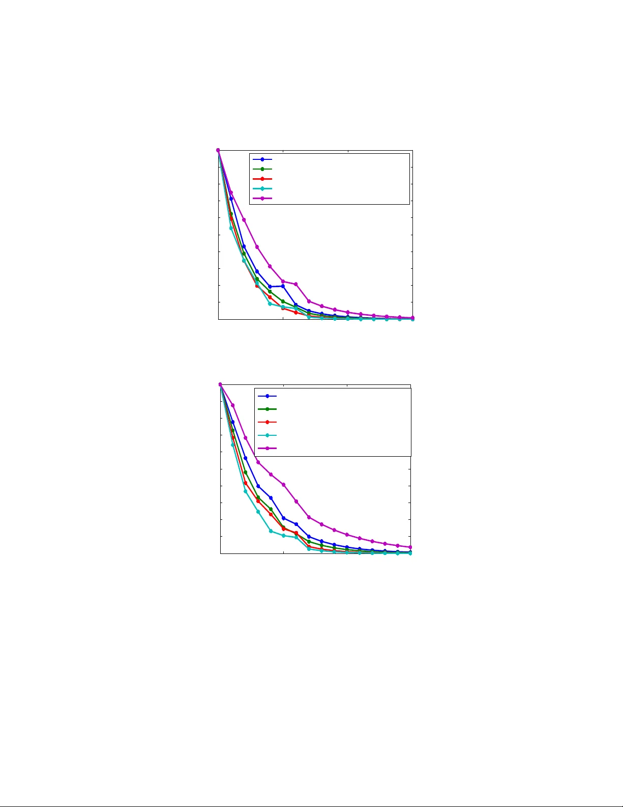
On The Blo c k Decomp osition and Sp ectral F actors of λ -Matrices Belk acem Bekhiti 1 ,Ab delhakim Dahimene 1 ,Kamel Hariche 1 and George F. F ragulis 2 1 Signal and System Lab oratory , Electronics and Electrotec hnics Institute Universit y of Boumerdes, Algeria, IGEE Ex:(INELEC) 2 W estern Macedonia Univ ercity of Applied Sciences, Kozani, Hellas. Marc h 29, 2018 Abstract In this paper w e factorize matrix polynomials in to a complete set of sp ectral factors using a new design algorithm and w e pro vide a complete set of blo c k ro ots (solv ents). The pro cedure is an extension of the (scalar) Horner metho d for the computation of the blo c k roots of matrix polyno- mials. The Blo ck-Horner metho d brings an iterative nature, faster con- v ergence, nested programmable scheme, needless of an y prior knowledge of the matrix p olynomial. In order to av oid the initial guess metho d w e prop osed a combination of tw o computational pro cedures . First w e start giving the right Blo c k- Q. D. (Quotient Differ enc e) algorithm for spectral decomp osition and matrix p olynomial factorization. Then the construc- tion of new blo ck Horner algorithm for extracting the complete set of sp ectral factors is given. Keyw ords: Blo ck ro ots; Solven ts; Sp ectral factors; Block-Q.D. algorithm; Blo c k-Horner’s algorithm; Matrix polynomial 1 In tro duction In the early da ys of control and system theory , frequency domain tec hniques w ere the principal tools of analysis, mo deling and design for linear systems. Dynamic systems that can be modeled b y a scalar m th order linear differential (difference) equation with constan t co efficien ts are amenable to this type of analysis see [[1]] and [[2]] - other references [[3]]. In the case of a single input - single output (SISO) system the transfer function is a ratio of tw o scalar p olynomials. The dynamic properties of the system (time response, stabilit y , etc.) dep end on the ro ots of the denominator of the transfer function or in other words on the solution of the underlying homogeneous differen tial equation (difference equation in discrete-time systems) [[4]],[[5]],[[6]] [[7]],[[8]],[[9]]. The denominator of suc h systems is a scalar p olynomial and its sp ectral characteristics dep end on the lo cation of its ro ots in the s-plane. Hence the factorization (ro ot finding) of scalar p olynomials is an important to ol of analysis and design for linear systems[[10]] . In the case of multi input - multi output (MIMO) systems the dynamics can be mo deled by high-degree coupled differen tial equations or l t h degree m th order v ector linear differen tial (difference) equations with matrix constan t co efficien ts. In this pap er, we treat the dynamic prop erties of multiv ariable systems us- ing the laten t ro ots and /or the sp ectral factors of the corresponding matrix p olynomial, following the research by a num b er of recent publications see [[11]], [[12]], [[13]], [[14]], [[15]], [[16]] and [[17]] . The algebraic theory of matrix polynomials has b een inv estigated b y Go- h b erg et al.[[18]], Dennis et al. [[19]], Denman [[20]],[[21]], Shieh et al. [[22]],[[23]], [[25]], [[26]] and Tsai et al.[[24]]. V arious computational algorithms [[19]], [[21]], [[18]], [[22]] and [[27]] are a v ailable for ev aluating the solven ts and sp ectral fac- tors of a matrix p olynomial. Recen t approac hes [[19]],[[28]],[[29]] are the use of the eigen v alues and eigen vectors of the block companion form matrix of the corresp onding matrix polynomial (the λ -matrices) to construct the solv ents of that matrix polynomial based in the use of solv ents. It is often inefficient to explicitly determine the eigenv alues and eigenv ectors of a matrix, which can b e ill conditioned and either non-defective or defective. On the other hand, without prior knowledge of the eigenv alues and eigenv ectors of the matrix, the Newton-Raphson metho d [[22]],[[30]] has b een successfully utilized for finding the solv ents, as well as the block-pow er metho d (Tsai et al.) [[24]] for finding the solven ts and sp ectral factors of a general nonsingular (monic or comonic)polynomial matrix. The matrix p olynomial must hav e distinct blo c k solv ents, and the con ver- gence rate of the pow er metho d depends strongly on the ratio of the t wo blo ck eigen v alues of largest magnitude [[31]]. There are numerous numerical metho ds for computing the blo c k roots of matrix p olynomials without any prior knowl- edge of the eigen v alues and eigen vectors of the matrix polynomial. The most efficien t and more stable one that giv e the complete set of solven t at time is the Q.D . (quotient-difference) algorithm. The use of the Q.D . algorithm for such purp ose has b een suggested b y K. Haric he [[32]]. The purp ose of this paper is to illustrate the so called Blo c k quotient- difference ( Q.D .) algorithm and extend the (scalar) Horner metho d to its blo ck form for the computation of the block roots of matrix p olynomial and the deter- mination of complete set of solven ts and sp ectral factors of a monic p olynomial, without an y prior kno wledge of the eigen v alues and eigenv ectors of the matrix. See also P athan and Collyer [[33]]) where there is a presentation on Horner’s metho d and its application in solving p olynomial equations by determining the lo cation of ro ots. The ob jectives of this pap er are described as follo ws: • Illustration and finalization of the Blo ck quotient-difference ( Q.D .) algo- rithm for spectral decomp osition and matrix p olynomial factorization. • Construction of a new blo c k-Horner array and blo ck-Horner algorithm for extracting the complete set of sp ectral factors of matrix polynomials. • Combined the ab ov e algorithms for fast con vergence, high stability and a voiding initial guess. 2 Preliminaries In this section w e giv e some background material. 2.1 Surv ey on matrix p olynomials Definition 2.1. Given the set of m × m c omplex matric es A 0 , A 1 , ..., A l , the fol lowing matrix value d function of the c omplex variable λ is c al le d a matrix p olynomial of de gr e e l and or der m : A ( λ ) = A 0 λ l + A 1 λ l − 1 + ... + A l − 1 λ + A l (1) Definition 2.2. The matrix p olynomial A ( λ ) is c al le d: i. Monic if is A 0 the identity matrix. ii. Comonic if A l is the identity matrix. iii. R e gular or nonsingular if det ( A ( λ )) 6 = 0 . iv. Unimo dular if det ( A ( λ )) is nonzer o c onstant. Definition 2.3. The c omplex numb er λ i is c al le d a latent r o ot of the matrix p olynomial A ( λ ) if it is a solution of the sc alar p olynomial e quation det ( A ( λ )) = 0 The nontrivial ve ctor p , solution of A ( λ i ) p = 0 m is c al le d a primary right latent ve ctor asso ciate d with λ i . Similarly the nontrivial ve ctor q solution of q T A ( λ i ) = 0 m is c al le d a primary left latent ve ctor asso ciate d with λ i . Remark 2.4. . If A ( λ ) has a singular le ading c o efficient ( A l ) then A ( λ ) has latent r o ots at infinity. F r om the definition we c an se e that the latent pr oblem of a matrix p olynomial is a gener alization of the c onc ept of eigenpr oblem for squar e matric es. Inde e d, we c an c onsider the classic al eigenvalues/ve ctor pr oblem as finding the latent r o ot/ve ctor of a line ar matrix p olynomial ( λI − A ) . We c an also define the sp e ctrum of a matrix p olynomial A ( λ ) as b eing the set of al l its latent r o ots (notation σ ( λ ) ). Definition 2.5. A right blo ck r o ot also c al le d solvent of λ -matrix A ( λ ) and is an m × m r e al matrix R such that: R l + A 1 R l − 1 + ... + A l − 1 R + A l = O m ⇔ A R ( R ) = l X i =0 A i R l − i = O m (2) While a left solv en t is an m × m real matrix L suc h that: L l + L l − 1 A 1 + ... + LA l − 1 + A l = O m ⇔ A L ( L ) = l X i =0 L l − i A i = O m (3) Remark 2.6. F r om [[34]] we have the fol lowing: • Solvents of a matrix p olynomial do not always exist. • Gener alize d right (left) eigenve ctors of a right (left) solvent ar e the gener- alize d latent ve ctors of the c orr esp onding matrix p olynomial Definition 2.7. : A matrix R (r esp e ctively: L ) is c al le d a right (r esp e ctively: left) solvent of the matrix p olynomial if and only if the binomial ( λI − R ) (r esp e ctively: ( λI − L ))divides exactly A ( λ ) on the right (r esp e ctively: left). F rom [[35],[36])],[37])],[38])] we hav e Theorem 2.8. Given a matrix p olynomial A ( λ ) = A 0 λ l + A 1 λ l − 1 + ... + A l − 1 λ + A l (4) a) The r eminder of the division of A ( λ ) on the right by the binomial ( λI − X ) is A R ( X ) b) The r eminder of the division of A ( λ ) on the left by the binomial ( λI − X ) is A L ( X ) Henc e ther e exist matrix p olynomials Q ( λ ) and S ( λ ) such that: A ( λ ) = Q ( λ )( λI − X ) + A R ( X ) = ( λI − X ) S ( λ ) + A L ( X ) (5) Corollary 2.9. The fundamental r elation that exist b etwe en right solvent (r e- sp e ctively: left solvent) and right (r esp e ctively: left) line ar factor: A R ( X ) = 0 iff A ( λ ) = Q ( λ )( λI − X ) A L ( X ) = 0 iff A ( λ ) = ( λI − X ) S ( λ ) (6) In reference [2] it is stated the following: Theorem 2.10. : Consider the set of solvents { R 1 , R 2 , ..., R l } c onstructe d fr om the eigenvalues ( λ 1 , λ 2 , ..., λ l ) of a matrix A c . { R 1 , R 2 , ..., R l } is a c omplete set of solvents if and only if:    ∪ σ ( R i ) = σ ( A c ) σ ( R i ) ∩ σ ( R j ) = ∅ det ( V R ( R 1 , R 2 , ..., R l )) 6 = 0 (7) Wher e: σ denotes the sp e ctrum of the matrix. V R V andermonde matrix c orr e- sp onding to { R 1 , R 2 , ..., R l } given as V R ( R 1 , R 2 , ..., R l ) =      I m I m ... I m R 1 R 2 ... R l . . . . . . ... . . . R l − 1 1 R l − 1 2 ... R l − 1 l      (8) Remark 2.11. : we c an define a set of left solvents in the same way as in the pr evious the or em. The r elationship b etwe en latent r o ots, latent ve ctors, and the solvents c an b e state d as fol lows: F rom [[39]] we hav e the follo wing: Theorem 2.12. :If A ( λ ) has n = ml line arly indep endent right latent ve ctors p ij ( i = 1 , · · · , l ) and ( j = 1 , · · · , m ) (left latent ve ctors q ij i = 1 , · · · , l and j = 1 , · · · , m ) c orr esp onding to latent r o ots λ ij then P i Λ i P − 1 i , ( Q i Λ i Q − 1 i ) is a right (left) solvent. Wher e: P i = [ p i 1 , p i 2 , ..., p im ] , ( Q i = [ q i 1 , q i 2 , ..., q im ] T ) and Λ i = diag ( λ i 1 , λ i 2 , · · · , λ im ) . Theorem 2.13. If A ( λ ) has n = ml latent r o ots λ i 1 , λ i 2 , · · · , λ im and the c orr esp onding right latent ve ctors p i 1 , p i 2 , ..., p im has as wel l as the left latent ve ctors q i 1 , q i 2 , ..., q im ar e b oth line arly indep endent, then the asso ciate d right solvent R i and left solvent L i ar e r elate d by: R i = W i L i W − 1 i Wher e: W i = P i Q i and P i = [ p i 1 , p i 2 , ..., p im ] , ( Q i = [ q i 1 , q i 2 , ..., q im ] T ). and ” T ” stands for tr ansp ose F or analysis and design of large-scale m ultiv ariable systems, it is necessary to determine a complete set of solven ts of the matrix p olynomial. Giv en the matrix polynomial A ( λ ) if a righ t solven t R is obtained, the left solven t of L of A ( λ ) associated with R can b e determined b y using the follo wing [[39]]: L = Q − 1 RQ rank( Q ) = m (9) Where Q is the solution of the following linear matrix equation [[39]]: l − 1 X i =0 R l − 1 − i QB i = I m (10) Or in v ector form using the Kronec ker pro duct w e hav e V ec ( Q ) =  l − 1 P i =0 B i T N  R l − 1 − i   − 1 V ec ( I m ) (11) Where: N designates the Kroneck er product, and B i are the matrix co efficien ts of B ( λ ) with λI m − R factored out from A ( λ ), i.e., B ( λ ) = A ( λ )  λI m − R  − 1 = l − 1 X i =0 B i λ l − 1 − i (12) B ( λ ) = B 0 λ l − 1 + B 1 λ l − 2 + ... + B l − 1 (13) W e can compute the coefficients B i , using the algorithm of synthetic division: B 0 = I m B 1 = B 0 A 1 + B 0 R · · · B k = B 0 A k + B k − 1 R k = 1 , 2 , ..., l − 1 O m = B 0 A l + B l − 1 R Theorem 2.14. If the elementary divisors of A ( λ ) ar e line ar, then A ( λ ) c an b e factor e d into the pr o duct of l -line ar monic λ -matric es c al le d a c omplete set of sp e ctr al factors. A ( λ ) = ( λI m − Q l )( λI m − Q l − 1 ) ... ( λI m − Q 1 ) (14) wher e: ( λI m − Q i ) , i = 1 ...l ar e r eferr e d to as a c omplete set of line ar sp e ctr al factors. The m × m c omplex matric es Q i , i = 1 ...l ar e c al le d the sp e ctr al factors of the λ -matrix A ( λ ) . The most right sp ectral factor Q 1 is a right solven t of A ( λ ) and the most left sp ectral factor Q l is a left solv ent of A ( λ ), whereas the sp ectral factors may or may not be solv ents of A ( λ ). The relationship b et ween solven ts and spectral factors are studied b y Shieh and Tsa y in reference [24]. 2.2 T ransformation of solven ts to sp ectral factors The diagonal forms of a complete set of solv ents and those of a complete set of sp ectral factors are identical and are related by similarity transformation. Theorem 2.15. :[[23]] Consider a c omplete set of right solvents { R 1 , R 2 , ..., R l } of monic λ -matrix A ( λ ) , then A ( λ ) c an b e factor e d as: A ( λ ) = N l ( λ ) = ( λI m − Q l )( λI m − Q l − 1 ) ... ( λI m − Q 1 ) By using the fol lowing r e cursive scheme: (for k = 1 , ..., l ) Q k =  N ( k − 1) R ( R k )  R k  N ( k − 1) R ( R k )  − 1 (15) wher e: N k ( λ ) = ( λI m − Q k ) N k − 1 ( λ ) k = 1 , ..., l (16) and for any j we write N kR ( R j ) = N ( k − 1) R ( R j ) R j − Q k N ( k − 1) R ( R j ) , k = 1 , ..., l with: N 0 ( λ ) = I m N 0 R ( R j ) = I m for any j and r ank ( N ( k − 1) R ( R k )) = m, k = 1 , ..., l Similarly the sp ectral factors can b e obtained from the known L i of A ( λ ) as follo w: (for k = 1 , ..., l ) Q k = Q l +1 − k (17) Q k =  M ( k − 1) L ( L k )  − 1 L k  M ( k − 1) L ( L k )  (18) where: M k ( λ ) = M k − 1 ( λ )( λI m − Q k ) k = 1 , ..., l (19) and for an y j we write M kL ( L j ) = L j M ( k − 1) L ( L j ) − M ( k − 1) L ( L j ) Q k , k = 1 , ..., l with: M 0 ( λ ) = I m M 0 L ( L j ) = I m for an y j rank( M ( k − 1) L ( L k )) = m k = 1 , ..., l M ( k − 1) L ( L i ) is a left matrix p olynomial of M ( k − 1) ( λ ) ha ving λ replaced by a left solv ent L j the spectral factorization of A ( λ ) b ecomes: A ( λ ) = M l ( λ ) = ( λI m − Q 1 )( λI m − Q 2 ) ... ( λI m − Q l ) 2.3 T ransformation of sp ectral factors to solv en ts Giv en a complete set of sp ectral factors of a λ -matrix A ( λ ), then a corresp onding complete set of righ t (left) solv ents can b e obtained. The transformation of sp ectral factors to righ t (left) solven ts of a λ -matrix can b e deriv ed as follo w [[23]]: Theorem 2.16. Given a monic λ -matrix with al l elementary devisors b eing line ar A ( λ ) = ( λI m − Q l )( λI m − Q l − 1 ) ... ( λI m − Q 1 ) wher e Q i ( , Q l +1 − i ) i = 1 , ..., l ar e a c omplete set of sp e ctr al factors of a λ - matrix A ( λ ) , and Q i T Q j = ∅ No w let us define λ -matrices N i ( λ ) i = 1 , ..., l as follo w: N i ( λ ) = ( λI − Q i ) − 1 N i − 1 ( λ ) (20) N i ( λ ) = I m λ l − i + A 1 i λ l − i − 1 + ... + A ( l − i − 1) i λ + A ( l − i ) i (21) with N 0 = A ( λ ) then the transformation matrix P i whic h transforms the sp ec- tral factor Q i ( , Q l +1 − i ) to the right solven t R i ( , R l +1 − i )of A ( λ ) can b e constructed from the new algorithm as follow: (rank( P i ) = m ) R i , R l +1 − i = P i Q i P i − 1 i = 1 , ..., l (22) where: the m × m matrix P i can b e solv ed from the following matrix equation i = 1 , ..., m V ec ( P i ) = ( G N i ( Q i )) − 1 V ec ( I m ) (23) where G N i ( Qi ) (rank( G N i ( Q i )) = m 2 ) is defined b y: G N i ( Q i ) , ( Q l − i i ) T N I m + ( Q l − i − 1 i ) T N A 1 i + ... + Q i T N A ( l − i ) i + I m N A ( l − i ) i in the same w ay the complete set of sp ectral factors Q i , i = 1 , 2 , ..., l can b e conv erted in to the left solven t L i , i = 1 , 2 , ..., l using the following algorithm: M i ( λ ) = M i − 1 ( λ )( λI m − Q i ) − 1 , i = 1 , ..., l (24) M i ( λ ) = I m λ l − i + A 1 i λ l − i − 1 + ... + A ( l − i − 1) i λ + A ( l − i ) i (25) H M i ( Q i ) , I m N Q l − i i + A T 1 i N Q l − i − 1 i + ... + A T ( l − i − 1) i N Q i + A T ( l − i ) i N I m V ec ( S i ) = ( H M i ( Q i )) − 1 V ec ( I m ) , rank( H M i ( Q i )) = m 2 L i = S − 1 i Q i S i i = 1 , ..., l (26) 2.4 Blo c k companion forms A useful to ol for the analysis of matrix p olynomials is the block companion form matrix. Given a λ -matrix as in eq(1) where A i ∈ C m × m and λ ∈ C , the asso ciated blo ck companion form matrices right (left) are: A R =         O m I m · · · O m O m O m · · · O m . . . . . . . . . O m O m O m . . . I m − A l − A l − 1 · · · − A 1         , A L =        O m · · · O m − A l I m · · · O m − A l − 1 . . . . . . . . . . . . O m · · · O m − A 2 O m · · · I m − A 1        (27) Note that: A L is the blo c k transp ose of A R . If the matrix p olynomial A ( λ ) has a complete set of solv ents, these companion matrices can b e resp ectiv ely blo c k diagonalised via the righ t(left) block V andermande matrix defined b y: V R =      I m I m · · · I m R 1 R 2 · · · R l . . . . . . . . . . . . R l − 1 1 R l − 1 2 · · · R l − 1 l      V L =      I m L 1 · · · L l − 1 1 I m L 2 · · · L l − 1 2 . . . . . . . . . . . . I m L l · · · L l − 1 l      (28) where R 1 , R 2 , ..., R l and/or L 1 , L 2 , ..., L l represen t the complete set of right (left) solv ents. Since the blo c k V andermande matrices are nonsingular [[ ? ]],[[ ? ]] and [[41]] w e can write V R − 1 A R V R = Blo c kdiag( R 1 , R 2 , ..., R l ) (29) V L − 1 A L V L = Blo c kdiag( L 1 , L 2 , ..., L l ) (30) These similarity transformations do a blo ck decoupling of the sp ectrum of A ( λ ) whic h is very useful in the analysis and design of large order control systems. 3 Sp ecial F ractorization Algorithms In this section we are going to presen t algorithms that can factorize a linear term from a given matrix polynomial. Firstly we give the generalized quotien t differ- ence algorithm and next we giv e a new extended algorithm based on the Horner sc heme. The matrix quotien t-difference Q.D . algorithm is a generalization of the scalar case [[42]] and it is developed in [[43]] The scalar Q.D . algorithm is used for finding the roots of a scalar p olynomial. The Quotient-Difference sc heme for matrix p olynomials can b e defined just like the scalar one [[10]] and it is consists on building a table that we call the Q.D . tableau. 3.1 The righ t blo c k matrix Q.D. algorithm Giv en a matrix p olynomial with nonsingular co efficien ts as in eq(1).The ob jec- tiv e is to find the sp ectral factors of A ( λ ) that will allow as write A ( λ ) as a pro duct of n -linear factors as in eq(1). The block left companion form, is: C 3 =        − A 1 I m · · · O m − A 2 O m · · · O m . . . . . . . . . . . . − A l − 1 · · · · · · I m − A l · · · · · · O m        (31) The required transformation is a sequence of LR decomp osition suc h that: C 3 =  C 11 C 12 C 21 C 22  =  I m O m X m I m   A B C D  (32) where: C 11 =        − A 1 I m · · · O m − A 2 O m · · · O m . . . . . . . . . . . . − A l − 2 · · · · · · I m − A l − 1 · · · · · · O m        , C 12 =        O m O m . . . O m I m        C 21 = [ − A l O m O m , ..., O m ] , C 22 = [ O m ] It is required to hav e C = 0, then let X = [ − X 1 X 2 X 3 , ..., X l − 1 ] (33) W e obtain the follo wing set of equations: X 1 A 1 + X 2 A 2 + ... + X l − 1 A l − 1 = A l X 1 = X 2 = ... = X l − 2 = 0 X l − 1 + D = 0 Leading the follo wing decomp osition of C 3 : C 3 =        I m · · · O m O m O m · · · O m O m . . . . . . . . . . . . O m · · · I m O m O m · · · A l A − 1 l − 1 I m               − A 1 I m · · · O m − A 2 O m · · · O m . . . . . . . . . . . . − A l − 1 O m · · · I m O m O m · · · − A l A − 1 l − 1        Hence C 3 can be written as: C 3 = L − ( l − 2) R − ( l − 2) (34) Con tinuing this pro cess of the block C 11 up when C 3 is equiv alent to a matrix R 0 C 3 = L − ( l − 2) L − ( l − 3) ...L 0 R 0 (35) R 0 =        − A 1 I m · · · O m O m O m − A 2 A − 1 1 · · · O m O m . . . . . . . . . . . . . . . O m O m · · · − A l − 1 A − 1 l − 2 I m O m O m · · · O m − A l A − 1 l − 1        (36) It is clear that if the matrices L 0 , L − 1 , ..., L l − 2 are iden tity matrices, then the blo c k companion matrix C 3 will be : M =        Q 1 I m · · · O m O m O m Q 2 · · · O m O m . . . . . . . . . . . . . . . O m O m · · · Q l − 1 I m O m O m · · · O m Q l        (37) The following theorem shows that under certain conditions, the sequence of L 0 , L − 1 , ..., L l − 2 con verges to identities see [[44]] and [[10]]: Theorem 3.1. L et M = X Λ X − 1 wher e Λ =      R 1 O m · · · O m O m R 2 · · · O m . . . . . . . . . . . . O m O m · · · R l      (38) If the fol lowing c onditions ar e satisfie d: a) dominanc e r elation b etwe en R k : R 1 > R 2 > ....R l b) X − 1 = Y has a Blo ck LR factorization L y R y c) X has a Blo ck LR factorization L x R x Then the blo ck LR algorithm just define d c onver ges (i.e. L k → I ) The ab o ve theorem states that we can start the Q.D . algorithm b y consid- ering: E 1 (0) = − A 2 A 1 − 1 , E 2 ( − 1) = − A 3 A 2 − 1 , E 3 ( − 2) = − A 4 A 3 − 1 , ..., E l − 1 − ( l − 2) = − A l A l − 1 − 1 Q 1 (0) = − A 1 , Q 2 ( − 1) = O m , ..., Q l − 1 − ( l − 2) = O m The last tw o equations pro vide us with the first tw o rows of the Q.D. tableau (one row of Q 0 s and one row of E 0 s ). Hence, w e can solve the rhombus rules for the bottom elemen t (called the south elemen t b y Henrici [[42]]). W e obtain the ro w generation of the Q.D. algorithm: ( Q i ( j +1) = Q i ( j ) + E i ( j ) − E i ( j +1) E i ( j +1) = Q i +1 ( j ) E i ( j )  Q i ( j +1)  − 1 (39) W riting this in tabular form yield where the Q i ( j ) are the spectral factors of A ( λ ) . In addition, the Q.D. algorithm gives all spectral factors simultaneously and in dominance order. W e ha ve c hosen, in the ab o ve, the ro w generation algorithm because it is numerically stable see reference [[10]] for details. Figure 1: * Q.D algorithm Example 3.2. Consider a matrix p olynomial of 2 nd or der and 3 nd de gr e e with the fol lowing matrix c o efficients. A 0 =  1 0 0 1  , A 1 =  − 27 . 1525 0 . 8166 − 179 . 7826 38 . 1525  A 2 =  116 . 4 85 . 0 1043 . 4 836 . 7  , A 3 =  126 . 9 353 . 5 1038 . 7 2947 . 6  We apply now the gener alize d r ow gener ation Q.D . algorithm to find the c om- plete set of sp e ctr al factors and then we use the similarity tr ansformations given by Shieh [[39]] to obtain the c omplete set of solvents b oth left and right e quations(19)-(26). Step 1: initialization of the pr o gr am to start Enter the de gr e e and the or der m = 2 , l = 3 Enter the numb er of iter ations N = 35 Enter the matrix p olynomial c o efficients A i Step 2: Construct Q 1 and E 1 the first r ow of Q 0 s and first r ow of E 0 s Q 1 = [ − A 1 A − 1 0 O 2 O 2 ] , E 1 = [ O 2 A 2 A − 1 1 A 3 A − 1 2 O 2 ] Step 3: Building or gener ating the r est r ows using the rhombus rules For n = 1 : N E 2 = [ ]; Q 2 = [ ]; For k = 1 : 2 : m ∗ l q 2 = ( E 1 ((: , k + 2 : k + 3) − E 1 (: , k : k + 1)) + Q 1 (: , k : k + 1); Q 2 = [ Q 2 , q 2 ]; End Q 2 ; For k = 1 : 2 : m ∗ l − 2 e 2 = ( Q 2 (: , k + 2 : k + 3))( E 1 (: , k : k + 1))( Q 2 (: , ( k : k + 1))) − 1 ; E 2 = [ E 2 , e 2 ]; End E 2 = [ O 2 , E 2 , O 2 ]; Q 1 = Q 2 ; E 1 = E 2 ; End Q 1 ; S 1 = Q 1 (: , 1 : 2) S 2 = Q 1 (: , 3 : 4) S 3 = Q 1 (: , 5 : 6) R unning the ab ove steps (1) to (3) we obtain the fol lowing c omplete set of sp e c- tr al factors S i : Q 1 =  3 . 0000 2 . 0000 − 8 . 2908 0 . 7118 32 . 4434 − 3 . 5284 − 90 . 000 − 15 . 000 − 16 . 8400 8 . 1248 286 . 6226 − 31 . 2773  S 1 =  3 . 0 2 . 0 − 90 . 0 − 15 . 0  , S 2 =  − 8 . 2908 0 . 7118 − 16 . 8400 8 . 1248  , S 3 =  32 . 4434 − 3 . 5284 286 . 6226 − 31 . 2773  Now, we should extr act a c omplete set of right solvent fr om those blo ck sp e ctr a using the algorithmic similarity tr ansformations in e quations fr om (21) to (24). Step 4: R everse the orientation of sp e ctr al factors U 1 = S 3 ; U 2 = S 2 ; U 3 = S 1 Step 5: Evaluate the c o efficients using the synthetic long division and then find the c orr esp onding tr ansformation matrix as in the or em 2.16. N 11 = A 1 + U 1 ; N 12 = A 2 + U 1 ? N 11 ; G 1 = ( U 2 1 ) T N I 2 + ( U 1 ) T N N 11 + I 2 N N 12 ; v ecp 1 = G − 1 1 ? [1; 0; 0; 1] p 1 = [ v ecp 1 (1 : 2) , v ecp 1 (3 : 4)]; R 1 = p 1 ? U 1 ? ( p 1 ) − 1 ; Y ou c an verify the first solvent using: rightzer o1 = A 0 ? ( R 1 ) 3 + A 1 ? ( R 1 ) 2 + A 2 ? R 1 + A 3 Step 6: r e do the same pr o c ess for the next right solvents N 21 = N 11 + U 2 ; G 2 = ( U 2 ) T N I 2 + I 2 N N 21 ; v ecp 2 = G ( 2 − 1) ? [1; 0; 0; 1] p 2 = [ v ecp 2 (1 : 2) , v ecp 2 (3 : 4)]; R 2 = p 2 ? U 2 ? ( p 2 ) − 1 ; F or verific ation also you c an use: rightzer o 2 = A 0 ? ( R 2 ) 3 + A 1 ? ( R 2 ) 2 + A 2 ? R 2 + A 3 Step 7: The last solvents ar e obtaine d dir e ctly fr om the most left sp e ctr al factor: R 3 = S 1 or by usinguse the tr ansformation: G 3 = ( I 2 ) T N I 2 ; v ecp 3 = G − 1 3 ? [1; 0; 0; 1] p 3 = [ v ecp 3 (1 : 2) , v ecp 3 (3 : 4)]; R 3 = p 3 ? U 3 ? p − 1 3 = U 3 ; The final r esults ar e : R 1 =  0 . 3637 − 4 . 5495 − 0 . 8183 0 . 8024  , R 2 =  7 . 2354 1 . 4024 1 . 2995 − 7 . 4015  , R 3 =  3 . 0000 2 . 0000 − 90 . 000 − 15 . 000  Final ly, we c an also obtain the c orr esp onding c omplete set of left solvents using the algorithmic similarity tr ansformation describ e d in e quations fr om (10) to (12). Step 8: c o efficients determination using the synthetic long division B 0 i = I 2 ; B 1 i = A 1 + R i ; B 2 i = A 2 + B 1 i ? R i ; Step 9: find the c orr esp onding similarity tr ansformation matrix as in e qua- tions fr om e quations (10) to (12). For i = 1 : l v ecQ i = (( B 0 i ) T O ( R i ) 2 + ( B 1 i ) T O R i + ( B 2 i ) T O I 2 ) − 1 ? [1; 0; 0; 1]; Q i = [ v ecQ i (1 : 2) , vecQ i (3 : 4)]; L i = ( Q i ) − 1 ? R i ? Q i ; Y ou can verify the left solvents using: Leftzero = L 3 i ? A 0 + L 2 i ? A 1 + L i ? A 2 + A 3 End The left solvents ar e now obtaine d: L 1 =  32 . 443 − 3 . 5284 286 . 622 − 31 . 2773  , L 2 =  25 . 1323 − 2 . 8370 204 . 5931 − 25 . 2983  , L 3 =  21 . 0123 − 4 . 6531 178 . 0910 − 33 . 0123  3.2 Extended Horner algorithm Horner’s metho d is a technique to ev aluate p olynomials quickly . It needs l mul- tiplications and l additions and it is also a nested algorithmic programming that can decomp ose a p olynomial into a multiplication of l linear factors (Horner’s metho d) based on the Euclidian syn thetic long division. Similarly Horner’s metho d is a nesting technique requiring only l multipli- cations and l additions to ev aluate an arbitrary l th -degree polynomial [[45]]. Theorem 3.3. L et the function P ( x ) b e the p olynomial of de gr e e l define d on the r e al field P : R → R wher e: a i ar e c onstant c o efficients and x is r e al variable. P ( x ) = a 0 x l + a 1 x l − 1 + ... + a l − 1 x + a l (40) If b 0 = a 0 and b k = a k + b k − 1 α, k = l , ..., 2 , 1 Then b l = P ( α ) and P ( x ) c an b e written as: P ( x ) = ( x − α ) Q ( x ) + b l (41) Wher e: Q ( x ) = b 0 x l − 1 + b 1 x l − 2 + ... + b l − 2 x + b l − 1 (42) Pr o of. The theorem can b e pro ved using a direct calculation. P ( x ) = a 0 x l + a 1 x l − 1 + ... + a l − 1 x + a l P ( x ) = ( x − α )( b 0 x l − 1 + b 1 x l − 2 + ... + b l − 2 x + b l − 1 ) + b l Iden tifying the co efficien ts of x with differen t p o wers w e get: b 0 = a 0 b 1 = a 1 + b 0 α . . . b k = a k + b k − 1 α where k = l, l − 1 , ..., 2 No w if α is a ro ot of the p olynomial P ( x ) , then b l should b e zero, and a l + b l − 1 α = 0 . Hence, w e may write α = −  a l b l − 1  or x k +1 = −  a l b l − 1 ,k  k = 0 , 1 , ... The algorithm of Horner metho d in its recursiv e formula is then: b i,k = a k + b i,k − 1 x k ; i = 1 , ..., l and b 0 ,k = a 0 No w we generalize this nested algorithm to matrix p olynomials, consider the monic λ -matrix A ( λ ) and according to theorem 2.8 the matrix A ( λ ) can b e factored as: A ( λ ) = Q ( λ )( λI − X ) + A R ( X ) (43) where A ( λ ) = A 0 λ l + A 1 λ l − 1 + ... + A l = l X i =0 A i λ l − i Q ( λ ) = B 0 λ l − 1 + B 1 λ l − 2 + ... + B l − 1 = l − 1 X i =0 B i λ l − i − 1 A R ( X ) = cst Using the algorithm of synthetic long division for matrices we obtain: B 0 = A 0 = I m B 1 = B 0 A 1 + B 0 X · · · B k = B 0 A k + B k − 1 X k = 1 , 2 , ..., l − 1 O m = B 0 A l + B l − 1 X F rom the last tw o equations we can iterate the pro cess to get recursiv e algo- rithm as follo w: Algorithm: Enter the number of iterations N For k = 0 : N Enter the degree and the order m, l Enter the matrix polynomial coef ficients A i X 0 = initial guess; For i = 1 : l B i,k = B 0 A i + B i − 1 ,k X k ; End X k +1 = −  B ( l − 1) ,k  − 1 B 0 A l ; X k = X k +1 ; End When y ou get the first sp ectral factor rep eat the pro cess until you get the complete set. Example 3.4. Consider a matrix p olynomial of 2 nd or der and 3 rd de gr e e with the fol lowing matrix c o efficients. A ( λ ) = A 0 λ 3 + A 1 λ 2 + A 2 λ + A 3 With A 0 =  1 0 0 1  , A 1 =  11 . 0000 − 1 . 0000 6 . 7196 17 . 0000  , A 2 =  30 . 0000 − 11 . 0000 70 . 9107 82 . 5304  , A 3 =  − 0 . 0000 − 30 . 0000 182 . 0000 89 . 8393  We apply now the extende d Horner’s metho d via its algorithmic version to find the c omplete set of sp e ctr al factors and then we use the similarity tr ansforma- tions given in [[23]] to obtain the c omplete set of left and right solvents The Blo ck Horner scheme is: When ( X 0 = O 2 ) :is an initial guess Initial starting value of iterations k = 0 and ( X 0 = O 2 ) η : tolerance error Giv en ξ where ξ ≥ η While ξ ≥ η A 0 =  1 0 0 1  A 1 =  11 . 0000 − 1 . 0000 6 . 7196 17 . 0000  B 0 = A 0 =  1 0 0 1  A 2 =  30 . 0000 − 11 . 0000 70 . 9107 82 . 5304  , ( B 1 ( k ) = B 0 A 1 + B 0 X k B 1 (0) =  11 . 000 − 1 . 0000 6 . 7196 17 . 000  A 3 =  − 0 . 0000 − 30 . 0000 182 . 0000 89 . 8393  , ( B 2 ( k ) = B 0 A 2 + B 1 ( k ) X k B 2 (0) =  30 . 0000 − 11 . 0000 70 . 9107 82 . 5304  X k +1 = − ( B 2 ( k )) − 1 B 0 A 3 ξ = 100 . k X k +1 − X k k k X k k X k = X k +1 k = k + 1 End R unning the ab ove algorithm we obtain the next c omplete set of sp e ctr al factors: S 1 =  0 . 00 1 . 00 − 3 . 25 2 . 00  , S 2 =  − 5 . 000 0 . 000 − 1 . 6042 − 7 . 000  S 3 =  − 6 . 000 − 0 . 000 − 1 . 8655 8 . 000  Final ly when we apply the similarity tr ansformation algorithm as in e quations fr om (21) to (24) to right (or left) solvent form we get: R 1 =  − 5 . 9574 0 . 2553 − 0 . 3404 − 8 . 0426  , R 2 =  − 4 . 9412 0 . 2941 − 0 . 4118 − 7 . 0588  R 3 =  0 . 000 1 − 3 . 25 − 2  3.2.1 Reformulation of the Blo c k Horner metho d An alternative form of the previous algorithm (under matrix and algebraic ma- nipulations is: B 0 ( k ) = A 0 = I m B 1 ( k ) = B 0 ( k ) A 1 + B 0 ( k ) X ( k ) ... B l − 1 ( k ) = B 0 ( k ) A l − 1 + B l − 2 ( k ) X ( k ) O m = B 0 ( k ) A l + B l − 1 ( k ) X ( k ) B l − 1 ( k ) = A l − 1 + ... + A 1 X l − 1 ( k ) + B 0 X l ( k ) ⇒ B l − 1 ( k ) = [ A R ( X k ) − A l ] X − 1 k ⇒ ( B l − 1 ( k )) − 1 = X k [ A R ( X k ) − A l ] − 1 Finally w e obtain the follo wing iterative formula: ( k = 0 , 1 , ... ) X k +1 = − ( B l − 1 ( k )) − 1 A l = X k [ A l − A R ( X k )] − 1 A l (44) Algorithm 3.5. Enter the de gr e e and the or der m, l Enter the matrix p olynomial c o efficients A i ∈ R m × m X 0 ∈ R m × m = initial guess; Give some smal l η and ( δ = initial start) > η k = 0 While δ ≥ η X k +1 = X k [ A l − A R X k ] − 1 A l ; δ = 100 . k X k +1 − X k k k X k k ; X k ← X k +1 ; k = k + 1; Con vergence condition: Using equations (44) w e obtain the conditions for the the algorithm to conv erge to the solution. 1. Upp er b ound eq(45) ⇔ X k +1 − X k = X k +1 A − 1 l A R ( X k ) eq(45) ⇔ k X k +1 − X k k = k X k +1 A − 1 l A R ( X k ) k eq(45) ⇔ k X k +1 − X k k ≤ k X k +1 k . k A − 1 l k . k A R X k k eq(45) ⇔ k X k +1 − X k k  k X k +1 k . k A − 1 l k  ≤ k A R ( X k ) k No w if X k tends to constan t matrix k X k k → M as k → ∞ and k X − 1 k k → N with k A − 1 l k = γ and k A l k = δ then: lim k →∞ k A R ( X k ) k ≥ k X ( k + 1) − X k k  k X ( k + 1) k . k A − 1 l k  ⇒ lim k →∞ k A R ( X k ) k ≥ ξ k γ .M (45) 2. L ower b ound A R ( X k ) = A l [ I − X − 1 k +1 X k ] = A l ( X k +1 ) − 1 [ X k +1 − X k ] ⇒ k A R ( X k ) k ≤ k A l k . k ( X k +1 ) − 1 k . k X k +1 − X k k ⇒ lim k →∞ k A R ( X k ) k ≤ δ.N ξ k (46) F rom eq. (45) and (46) w e obtain: ξ k γ .M ≤ lim k →∞ k A R ( X k ) k ≤ δ.N ξ k (47) Finally if the matrix X k tends to constan t matrix X k → S and ( A l − A R ( X k )) is nonsingular matrix then S is a solv ent of the matrix p olynomial A R ( S ) = O m . Con vergence Type: T o get the conv ergence type we should ev aluate a ratio relationship betw een any tw o successive differences. X k +1 − S = X k ([ A l − A R ( X k )] − 1 A l − I ) + X k − S (48) W e define F ( X k ) = ([ A l − A R ( X k )] − 1 A l − I ) then w e hav e: k X k − S k − k X k F ( X k ) k ≤ k X k +1 − S k ≤ k X k − S k + k X k F ( X k ) k (49) W e know that: lim k →∞ k X k F ( X k ) k = lim k →∞ ∆ k = ξ (50) from equations (49) and (50) we deduce that: 1 − ∆ k k X k − S k ≤ k X k +1 − S k k X k − S k ≤ 1 + ∆ k k X k − S k Finally: lim k →∞ k X k +1 − S k k X k − S k = 1 (51) Example 3.6. c onsider the fol lowing matrix p olynomial with r ep e ate d sp e ctr al factor: A ( λ ) =  λI −  − 7 . 1230 − 6 . 3246 5 . 9279 5 . 1230   2 = A 0 λ 2 + A 1 λ + A 2 With A 0 =  1 0 0 1  , A 1 =  14 . 2461 12 . 6493 − 11 . 8557 − 10 . 2461  A 2 =  13 . 2461 12 . 6493 − 11 . 8557 − 11 . 2461  Find X such that A R ( X ) = O 2 A R ( X ) = A 0 X 2 + A 1 X + A 2 If we apply the Blo ck Horner algorithm we find X 1 =  − 2 . 7323 − 1 . 8068 1 . 6798 0 . 7521  , X 2 =  − 11 . 5138 − 10 . 8424 10 . 1759 9 . 4939  Remark 3.7. The Pr op ose d Horner algorithm finds the whole set of sp e ctr al factors if it exists, even if ther e is no dominanc e factor among them. 3.2.2 Crossbred Newton Horner metho d In order to accelerate the Block Horner metho d w e make a crossbred (Hybrid) Generalized Newton algorithm which is v ery fast due to its restricted lo cal nature (i.e. Quadratic con vergence). Horner iteration Newton iteration X k +1 − X k = X k +1 A − 1 l A R ( X k ) , X k +1 − X k = − J − 1 ( X k ) A R ( X k ) Com bine them we get: X ( k +1 = X k + ( X k − J − 1 ( X k ) A R ( X k )) A l − 1 A R ( X k ) (52) where J ( X k ) is the F rec het differential. Definition 3.8. L et B 1 and B 2 b e Banach sp ac es and A R a nonline ar op er ator fr om B 1 to B 2 . If ther e exists a line ar op er ator L fr om B 1 to B 2 such that: B 1 → B 2 H → L ( X + H ) Wher e: k A R ( X + H ) − A R ( X ) − L ( X + H ) k = O ( k H k ) X, H ∈ B 1 A R ( X ) , L ( X + H ) ∈ B 2 Then L ( X + H ) is c al le d the F r e chet derivative of A R at X and sometimes is written dA R ( X, H ) . A lso is r e ad the F r e chet derivative of A R at X in the dir e ction H . And J ( X k ) .H = L ( X + H ) Algorithm Begin Enter the degree and the order m, l Enter the matrix polynomial coef ficients A i ∈ R m × m X 0 ∈ R m × m = initial guess; Gi ve initial J ( X 0 ) ∈ R m × m Gi ve some small η and ( δ =initial start) > η k = 0 While δ ≥ η X k +1 = X k ( I m + A l − 1 A R ( X k )) − J − 1 ( X k ) A R ( X k ) A l − 1 A R ( X k ); H k = X k +1 − X k ; J ( X k ) = ( A R ( X ( k + 1)) − A R ( X k )) H k − 1 ; δ = 100 . k X k +1 − X k k k X k k ; X k ← X k +1 ; k = k + 1; End 3.2.3 Two sta ge Block Horner algorithm T o accelerate the blo c k Horner algorithm we use now a t wo stage Newton like iteration. No w by using theorem 2.8 w e obtain: A R ( X ) = ( X − Θ)( X l − 1 + B 1 X l − 2 + ... + B l − 1 ) + B l ⇒ A R ( X ) = ( X − Θ) Q ( X ) + B l ⇒ X − Θ = ( A R ( X ) − B l ) Q − 1 ( X ) where Q ( X ) = X l − 1 + B 1 X l − 2 + ... + B l − 1 and A R (Θ) = B l No w if Θ is a solv ent then B l = O m If no w assume that Θ = X k +1 is a solv ent to the matrix p olynomial A R then A R ( X k +1 ) = O m and X k +1 = X k − A R ( X k ) Q − 1 ( X k +1 ). Set also Q ( X ) = ( X − Θ)( X l − 1 + C 1 X l − 2 + ... + C l − 2 ) + C l − 1 F rom the Horner sc heme we can ev aluate b oth B i and C i recursiv ely: B 0 = I m B 1 = A 1 + B 0 X C 0 = I m B 2 = A 2 + B 1 X C 1 = B 1 + C 0 X ... C 2 = B 2 + C 1 X B l − 1 = A l − 1 + B l − 2 X ... O m = B l = A l + B l − 1 X = A R ( X ) C l − 1 = B l − 1 + C l − 2 X = Q ( X ) After iterating the last equation we get : After iterating the last equation w e get : B l ( k ) = A l + B l − 1 ( k ) X k C l − 1 ( k ) = B l − 1 ( k ) + C l − 2 ( k ) X k B l ( k ) = A R ( X k ) C l − 1 ( k ) = Q ( X k ) Algorithm: X 0 = initial guess, ( B 0 = C 0 = I ) ∈ R m × m enter small enough number η (T olerance error) ( δ =initial start) > η enter the set of m × m ( A 0 , A 1 , ..., A l ) matrices k = 0 While δ > η For i = 1 : 1 : l B i ( k ) = A i + B i − 1 ( k ) X k End For i = 1 : 1 : l − 1 C i ( k ) = B i ( k ) + C i − 1 ( k ) X k End X k +1 = X k − B l ( k )( C l − 1 ( k )) − 1 δ = 100 . k X k +1 − X k k 2 k X k k 2 X k ← X k +1 k ← k + 1 End Remark 3.9. this two stage algorithm gathers the two advantages of Horner sachem and Newton algorithm b e c ause it is neste d pr o gr ame d natur e, lar ge sense indep endenc e on initial c onditions and faster in exe cution due to the likeness or the c onformity to Newton metho d. Example 3.10. Given the fol lowing matrix p olynomial A R ( X ) = A 0 X 3 + A 1 X 2 + A 2 X + A 3 Wher e: A 0 =  1 0 0 1  , A 1 =  12 . 8793 − 0 . 4881 − 2 . 0989 15 . 1207  A 2 =  56 . 5645 − 8 . 7887 10 . 2686 55 . 9659  , A 3 =  95 . 9331 − 37 . 5549 160 . 9539 − 6 . 0938  We apply the two stage Horner algorithm and after 15 iter ations we get: X 0 =  5 . 2114 4 . 8890 2 . 3159 6 . 2406  , X 1 =  − 3 . 0729 1 . 4058 − 4 . 6569 1 . 0730  With A R ( X 15 ) =  − 0 . 0081 0 . 0106 0 . 0265 0 . 0145  3.2.4 Reformulation of the tw o stage Blo c k Horner method After back substitution of the nested programmed scheme and accum ulation we obtain: B l ( k ) = A R ( X k ) and C l − 1 ( k ) = lX k l − 1 + l − 1 A 1 X k l − 2 + ... + A l − 1 = ∆( X k ) The tw o stage Block Horner V arian algorithm can be obtained when w e use the compact forms of the matrices B l ( k ) and C l − 1 ( k ) in term of A R lead us to Newton lik e iterated pro cess. Algorithm: X 0 = initial guess Enter small enough number η (T olerance error) and ( δ = initial start) > η Enter the set of m × m ( A 0 , A 1 , ..., A l ) matrices k = 0 For i = 0 : 1 : l − 1 ∆ i = ( l − i ) A i End While δ > η A R ( X k ) = A 0 X k l + A 1 X k l − 1 + ... + A l ∆( X k ) = ∆ 0 X k l − 1 + ∆ 1 X k l − 2 + ... + ∆ l − 1 X k +1 = X k − A R ( X k )(∆( X k )) − 1 δ = 100 . k X k +1 − X k k 2 k X k k 2 X k ← X k +1 k ← k + 1 End 3.3 Commen ts • A n umerical method for solving a given problem is said to b e lo cal if it is based on lo cal (simpler) mo del of the problem around the solution. F rom this definition, we can see that in order to use a lo cal method, one has to pro vide an initial appro ximation of the solution. This initial approxima- tion can b e provided b y a global metho d. As shown in Dahimene [[10]], lo cal metho ds are fast conv erging while global ones are quite slow. This implies that a goo d strategy is to start solving the problem by using a global method and then refine the solution b y a lo cal metho d. • The prop osed h ybrid or tw o stage Blo c k-Horner’s algorithm conv erges rapidly as it p erforms a recursive iteration and is easily implemen ted in a digital computer. Horner’s algorithm could be used for ev aluation of solv ents of a matrix p olynomial, but this metho d depends largely upon the initial guess ev en in some cases the initial v alue of X k is randomly c hosen. Hence in sometimes it is very hard to find suitable solutions. Our Q.D . algorithm is numerically more stable and its initial starting v alues are w ell defined and ev aluated. • The complete program starts with the Q.D . algorithm. It is then follow ed b y a refinement of the righ t factor by Horner’s algorithm. After deflation, Horners algorithm is again applied using the next Q output from the Q.D . algorithm and the pro cess is rep eated un til w e find a linear term. The ab o ve process can b e applied only to p olynomial matrices that satisfy the conditions of theorem (i.e. complete right and left factorization and complete dominance relation betw een solv ents). • Many research w orks hav e b een done on the spectral decomp osition for matrix p olynomials to achiev e complete factorization and reconstruction of the block ro ots using algebraic and geometric numerical approaches, but (to our knowledge) nothing has been done for Blo ck-Horner’s algorithm and/or Block- Q.D. algorithm. 4 Application in con trol engineering The system under examination is a pow er plan t gas turbine (GE MS9001E) with single shaft, used as an electricity generator, installed in p o w er station unit Sonelgaz at M’SILA, Algeria. The dynamic mo del of this gas turbine obtained via MIMO Recursiv e Least square estimator, using experimental inputs/outputs data acquired on-site and the obtained mo del is of order n =6 with t wo inputs: (Output Pressure Compressor (OPC), and Output T emp erature Compressor (OTC)), and t wo outputs: (Exhaust T emp erature and Rotor Sp eed) [[46]]. In figure 2, the fundamen tal components of the system under study are given . Power Generation Rotor Speed OPC OTC Combustor Air Inlet GCV Fuel Gas Exhaust T emperature Axial Compressor T urbine Lancer Alternator Coupling Lner/Comp Coupling T urb/Alter Figure 2: sc hematic The dynamic model of this p o wer plant gas turbine is a linear time inv ari- an t m ulti input multi output system,describ ed by a set of high degree coupled v ector differential equations with matrix constan t coefficients(or a matrix trans- fer function). In our case the relationship b et ween the input and output is a ratio of t wo matrix p olynomials, expressed as a righ t (or left) matrix fraction description (RMFD or LMFD):  H ( λ ) = N R ( λ ) D R − 1 ( λ ) = D L − 1 ( λ ) N L ( λ ) (53) where: N R , D R , N L and D L are m atrix p olynomials and λ stands for the  d dt  op erator. see [[4]],[[40]] and [[48]] and the reference therein . The obtained λ - matrix transfer function of the p o wer plan t gas turbine system is: H ( λ ) = N ( λ ) D ( λ ) − 1 =  H 11 ( λ ) H 12 ( λ ) H 21 ( λ ) H 22 ( λ )  Where H 11 ( λ ) =  34 . 01 λ 5 − 116 . 9 λ 4 − 221 . 2 λ 3 − 102 . 5 λ 2 − 1 . 955 × 10 4 λ − 2077 λ 6 − 30 . 41 λ 5 − 45 . 33 λ 4 + 515 . 1 λ 3 − 1343 λ 2 + 1 . 805 × 10 4 λ + 9102  H 21 ( λ ) =  36 . 58 λ 5 − 42 . 7 λ 4 + 696 λ 3 + 3295 λ 2 − 208 . 4 λ + 1 . 979 × 10 4 λ 6 − 30 . 41 λ 5 − 45 . 33 λ 4 + 515 . 1 λ 3 − 1343 λ 2 + 1 . 805 × 10 4 λ + 9102  H 12 ( λ ) =  27 . 37 λ 5 − 53 . 9 λ 4 + 12 . 19 λ 3 − 767 . 4 λ 2 − 7918 λ − 8267 λ 6 − 30 . 41 λ 5 − 45 . 33 λ 4 + 515 . 1 λ 3 − 1343 λ 2 + 1 . 805 × 10 4 λ + 9102  H 22 ( λ ) =  32 . 93 λ 5 − 66 . 88 λ 4 + 1 . 5 λ 3 − 1474 λ 2 − 8675 λ − 1 . 675 × 10 4 λ 6 − 30 . 41 λ 5 − 45 . 33 λ 4 + 515 . 1 λ 3 − 1343 λ 2 + 1 . 805 × 10 4 λ + 9102  W e try to decouple the p o wer plant gas turbine dynamic mo del. Let us first factorize ( de c omp ose ) the n umerator matrix polynomial N ( λ ) into a complete set of sp ectral factors, then we use those blo ck zeros into the denominator D ( λ ) via state feedbac k. Hence the decoupling ob jectiv es are ac hieved. Consider the square matrix transfer function: H ( λ ) = N ( λ ) D − 1 ( λ ) =  k P i =0 N i λ i   l P i =0 D i λ i  − 1 = ( N k λ k + ... + N 1 λ + N 0 )( D l λ l + ... + D 1 λ + D 0 ) − 1 with: D l = I is an m × m identit y matrix and N i ∈ R m × m , ( i = 0 , 1 , ..., k ) D i ∈ R m × m , ( i = 0 , 1 , ..., l ), l > k Assume that N ( λ ) can b e factorized in to k Blo c k zeros and D ( λ )can b e factor- ized in to l Blo ck ro ots ( using one of the pr op ose d algorithms ): N ( λ ) = N k ( λI − Z 1 ) ... ( λI − Z k ) (54) D ( λ ) = ( λI − Q 1 ) ... ( λI − Q l ) . (55) The matrix transfer function can b e written : H ( λ ) = C ( λI − A ) − 1 B . Also via the use of state feedback the con trol law b ecomes a state dep enden t and b e rewritten as u ( t ) = − K.X ( t ) + F .r ( t ). Hence we obtain the follo wing closed lo op system: ( H ( λ )) closed = C ( λI − A + B K ) − 1 B F = N ( λ ) D − 1 d ( λ ) F where: D d ( λ ) = ( λI − Q d 1 ) ... ( λI − Q dl ) and Q di : are the desired sp ectral factors to be placed H ( λ ) closed = N ( λ ) D − 1 d ( λ ) F Hence, the closed loop matrix transfer function is of the form: H ( λ ) closed = N k ( λI − Z 1 ) ... ( λI − Z k )( λI − Q dl ) − 1 ... ( λI − Q d 1 ) − 1 F (56) In order to ac hiev e p erfect block decoupling w e choose: Q d 1 = N k J 1 N − 1 k , ..., Q d ( l − k ) = N k J ( l − k ) N − 1 k Q d ( l − k +1) = Z 1 , ..., Q dl = Z k J i = diag ( λ i 1 , ..., λ im ) , F = ( N k ) − 1 No w by assigning those blo c k ro ots the system is decoupled and the closed lo op matrix transfer function is: H ( λ ) closed = ( λI − J 1 ) − 1 ... ( λI − J l − k ) − 1 (57) No w we should construct the numerator and denominator matrix p olynomials of the gas turbine system from the matrix transfer function (see [[13],[14] and [17]]):  D ( λ ) = D 3 λ 3 + D 2 λ 2 + D 1 λ + D 0 , D 3 = I 2 N ( λ ) = N 3 λ 3 + N 2 λ 2 + N 1 λ + N 0 , N 3 = O 2 where:       D 0 D 1 D 2       =         − 37 . 0170 28 . 2888 − 223 . 8750 − 74 . 7887 34 . 8029 20 . 9798 − 280 . 2609 − 216 . 8345 − 14 . 0378 − 7 . 5183 − 12 . 3898 − 16 . 3740             N 0 N 1 N 2     =         211 . 7886 61 . 4727 331 . 6250 199 . 1758 100 . 8960 74 . 4572 148 . 1818 120 . 4265 34 . 0105 27 . 3669 36 . 5764 32 . 9324         Let w e decompose the n umerator and denominator matrix polynomials and re- construct their block roots: N ( λ ) = N 2 ( λI − Z 1 )( λI − Z 2 ) and D ( λ ) = ( λI − Q 1 )( λI − Q 2 )( λI − Q 3 ) The Blo c k sp ectral factors are approximately computerized with a residual normed tolerance error giv en b y: ε i = k Z i ∗ k − k Z i k k Z i ∗ k i = 1 , 2 . and ξ i = k Q i ∗ k − k Q i k k Q i ∗ k i = 1 , 2 , 3 Remark 4.1. The last Blo ck p ole Q 3 c an b e c onstructe d using the synthetic long division. Figur e (3) il lustr ates a c omp arison b etwe en the pr op ose d algorithms in term of the c onver genc e sp e e d and r esidual norme d tolr anc e err or. The n umerator blo c k zeros are computed using the prop osed algorithms compared to recen t developed metho d called the generalized secant metho d [[49]] whic h can factorize matrix polynomial into a complete set of blo c k ro ots. Numerical results of the developed pro cedures as illustrated in [[49]] give: N ( Z i ) = O 2 ⇒ Z 1 =  24 . 7235 23 . 1394 − 27 . 4494 − 24 . 9281  , Z 2 =  − 18 . 5711 − 16 . 0841 16 . 1166 13 . 4353  0 5 10 15 0 0.1 0.2 0.3 0.4 0.5 0.6 0.7 0.8 0.9 1 1 st Block Pole Q 1 Number of iterations Residual Norm ξ 1 The Block QD algorithm The Block Horner algorithm The Newton−Horner algorithm The Two stage algorithm The Secant algorithm 0 5 10 15 0 0.1 0.2 0.3 0.4 0.5 0.6 0.7 0.8 0.9 1 2 nd Block Pole Q 2 Number of iterations Residual Norm ξ 2 The Block QD algorithm The Block Horner algorithm The Newton−Horner algorithm The Two stage algorithm The Secant algorithm 0 5 10 15 0 0.1 0.2 0.3 0.4 0.5 0.6 0.7 0.8 0.9 1 1 st Block Zero Z 1 Number of iterations Residual Norm ε 1 The Block QD algorithm The Block Horner algorithm The Newton−Horner algorithm The Two stage algorithm The Secant algorithm 0 5 10 15 0 0.1 0.2 0.3 0.4 0.5 0.6 0.7 0.8 0.9 1 2 nd Block Zero Z 2 Number of iterations Residual Norm ε 2 The Block QD algorithm The Block Horner algorithm The Newton−Horner algorithm The Two stage algorithm The Secant algorithm Figure 3: The Residual Error Norm comparison study Although the Block Newton metho d aims to impro ve the conv ergence sp eed o ver the Block Horner metho d, it cannot alw ays ac hieve this goal. The Newton- Horner’s metho d conv erges quadratically due to its conformity to Newton metho d. As a consequence, the num b er of significant v alues is roughly doubled every it- eration, provided that X i is close to the ro ot ( ε = 0 . 521 × 10 − 4 ). The t w o stage algorithm is the best metho d of finding roots, it is simple and fast (at first sev en iterations the a verage error b ecomes ε = 0 . 213 × 10 − 3 and ξ = 0 . 341 × 10 − 3 ). The only dra wback of the tw o stage metho d is that it uses the matrix inv er- sion, and partially is dep endent on the initial guess. Our refinement algorithm a voided this obstacle. As indicated in figure (2) the Q-D algorithm con verges, but it is of global nature with no initial indep endence. The global con vergence c haracteristics of the secan t metho d are po or, as indicated in this figure. The desired denominator is of third order written in the form: D d ( λ ) = D d 3 λ 3 + D d 2 λ 2 + D d 1 λ + D d 0 Using the prescribed decoupling algorithm we obtain: F = N 2 − 1 , J 1 =  − 1 0 0 − 2  Q d 1 = N 2 − 1 J 1 N 2 − 1 , Q d 2 = Z 1 , Q d 3 = Z 2 D d ( λ ) = ( λI − Q d 1 )( λI − Q d 2 )( λI − Q d 3 ) = I λ 3 + D d 2 λ 2 + D d 1 λ + D d 0 Where: D d 2 = − ( Q d 1 + Q d 2 + Q d 3 ) =  − 13 . 5596 − 14 . 6249 21 . 7809 21 . 8999  D d 1 = ( Q d 1 Q d 2 + Q d 1 Q d 3 + Q d 2 Q d 3 ) =  − 126 . 4282 − 121 . 5061 161 . 6710 152 . 4741  D d 0 = − ( Q d 1 Q d 2 Q d 3 ) =  − 178 . 9732 − 164 . 0512 223 . 2851 202 . 6227  The state feedback gain matrix of the Blo c k con troller form is obtained by see [[47]],[[48]]: K ci = D di − D i With i = 0 , 1 , 2 and K c = [ K c 0 , K c 1 , K c 2 ] No w let we go bac k to original base by similarity transformation T c as found in [[4]],[[40]] and [[48]]: K = K c T c =  − 0 . 7616 − 3 . 2690 3 . 5737 − 0 . 0716 − 2 . 3462 1 . 4801 3 . 0439 5 . 4047 − 2 . 3853 2 . 4117 4 . 2560 0 . 0494  The new model of the decoupled system after state feedbac k is: A d = ( A − B K ) , B d = B F , and C d = C H ( λ ) closed = C ( λI − A + B K ) − 1 B F = N ( λ ) D − 1 d ( λ ) F =    1 λ + 1 0 0 1 λ + 2    Based on the results we deduce that the Block roots are w ell computed, b oth n umerator and denominator matrix p olynomials ( N ( λ ) and D ( λ )) are perfectly decomp osed using the prop osed procedure. 4.1 Suggestions for further researc h The results obtained during this research work arose man y questions and prob- lems whic h are sub ject for future researc h • Finding other globalization techniques for the Blo c k-Horner’s algorithm to a void the lo cal restriction and the problem of initial guess, so to arriv e at v ery fast global nested program. Also exploring and extending other scalar n umerical metho ds to factorize matrix p olynomials. • Both of The Blo c k-Horner’s algorithm and the Block- Q.D. algorithm as used in our w ork con verges to factors of a matrix polynomial. By using the defined similarity transformations, we can derive the solven ts. Ho wev er, it would be con venien t to ha ve a global algorithm that conv erges rapidly and directly to all solven ts. • If a column in the Q.D . tableau conv erges, it implies that there exists a factorization of the matrix polynomial that splits the spectrum in to a dominan t set and a dominated one. If the system under consideration is a digital system, we know that the largest modulus laten t roots affect the dynamic prop erties of the system. In such case, the Q.D . algorithm can b ecome a to ol for system reduction (using the dominant mode concept). • The computational pro cedure for finding the solven ts of a matrix p olyno- mial with rep eated blo c k ro ots (solven ts) and/or sp ectral factors need to b e inv estigated further. 5 Conclusion In this paper we ha v e introduced new numerical approaches for determining the complete sets of spectral factors and solven ts of a monic matrix polyno- mial. F or a voiding the initial guess we ha ve prop osed a systematic metho d for the Blo c k-Horner’s algorithm via a refinemen t of the Blo c k- Q.D . algorithm. A t least three adv antages are offeedr by the prop osed technique: (i) an algorithm with global nature is obtained; hence there is no initial-guess problem during the whole pro cedure, (ii) high speed conv ergence to each solution and only a few iterations are required (iii) via the help of refinement and direct cascading, the algorithms are easily coupled together and the whole sc heme is suitable for programming in a digital computer digital. The obtained solv ents can b e con- sidered as a useful to ol for carrying out the blo c k partial fraction expansion for the inv erse of a matrix p olynomial. Those partial fractions are matrix transfer functions of reduced order linear systems suc h that the realization of them leads to block diagonal (block-decoupling) or parallel decomp osed m ultiv ariable linear time in v ariant system. The dynamic prop erties of MIMO systems depend on blo c k p ole of its characteristic matrix p olynomial. Therefore they can b e used as to ols for blo c k-p ole placemen t, blo ck-system identification and blo c k-mo del order reduction. In addition, the proposed method can b e emplo yed to carry out the block sp ectral factorization of a matrix polynomial for problems in optimal con trol, filtering and estimation. Ac kno wledgemen t Dr. George F. F ragulis w ork is supp orted b y the program Rescom 80159 of the Univ. of Applied Science of W estern Macedonia, Hellas. References [1] J. J. DiStefano, A. R. Stubberud, I. J. Williams, The ory and Pr oblems of F e e db ack and Contr ol Systems , Mc. Gra w Hill, 1967. [2] B. N. P arlett, The LU and QR Algorithms , in Ralston and Wilf, Math- ematical Methods for Digital Computers, V ol. 2, John Wiley , 1967. [3] Bachir Nail, Ab dellah Kouzou,Ahmed Hafaifa, Par ametric Identific ation of Multivariable Industrial System Using L eft Matrix F r action Descrip- tion , J. Automation and Systems Engineering 10-4 (2016): 221-230 [4] Malik a Y aici, Kamel Hariche, On eigenstructur e assignment using blo ck p oles plac ement , European Journal of Control, May 2014. [5] Malik a Y aici, Kamel Haric he,Clark Tim, A Contribution to the Polyno- mial Eigen Pr oblem , In ternational Journal of Mathematics, Computa- tional, Natural and Ph ysical Engineering, V ol:8 No 10, 2014. [6] Nicholas J. Higham, F unction of Matric es: the ory and c omputation ,SIAM 2008. [7] George F. F ragulis T r ansformation of a PMD into an implicit system using minimal r e alizations of its tr ansfer function matrix in terms of finite and infinite sp e ctr al data , Journal of the F ranklin Institute, v ol.333, pages 41-56, 1996. [8] George F. F ragulis Gener alize d Cayley-Hamilton the or em for p olynomial matric es with arbitr ary de gr e e , In ternational Journal of Control, vol.62, pages 1341-1349, 1995. [9] B.G. Mertzios and George F. F ragulis The fundamental matrix in ARMA systems , IEEE International Conference on Industrial T echnology , pages 1541-1542, 2004. [10] A.Dahimene, Algorithms for the factorization of matrix p olynomials , Master Thesis INELEC , 1992. [11] A.Dahimene, Inc omplete matrix p artial fr action exp ansion , Con trol and Cyb ernetics vol. 38 (2009) No.3 [12] S. M. Ahn, Stability of a Matrix Polynomial in Discr ete Systems , IEEE trans. on Auto. Con tr., V ol. AC-27, pp. 1122-1124, Oct. 1982. [13] C. T. Chen, Line ar System The ory and Design , Holt, Reinhart and Win- ston, 1984. [14] T. Kailath, W. Li, Line ar Systems ,Pren tice Hall, 1980. [15] V. Kucera, Discr ete Line ar Contr ol: The Polynomial Equation Ap- pr o ach ,John Wiley , 1979. [16] P . Resende, E. Kaskurewicz, A Sufficient Condition for the Stability of Matrix Polynomials ,IEEE trans, on. Auto. Contr., V ol. A C-34, pp. 539- 541, Ma y 1989. [17] Leang S. Shieh, F. R Chang, B. C. Mcinnis, The Blo ck p artial fr action exp ansion of a matrix fr action description with r ep e ate d blo cl p oles , IEEE T rans. Auto. Cont. AC-31, pp. 236-239, 1986. [18] E. D. Denman and A. N. Beav ers, The matrix sign function and c ompu- tations in systems ,Appl. Math. Comput. 2:63-94 (1976). [19] M. K. Solak, Divisors of Polynomial Matric es: The ory and Applic a- tions ,IEEE trans. on Auto. Contr., V ol. A C-32, pp. 916-919, Oct. 1987. [20] J. E. Dennis, J. F. T raub, and R. P . W eb er, Algorithms for solvents of matrix p olynomials ,SZAhlJ. Numer. Anal. 15:523-533 (1978). [21] E. D. Denman, Matrix p olynomials, r o ots, and sp e ctr al factors , A &. Math. Comput. 3:359-368, (1977). [22] L. S. Shieh, S. Sac heti, A Matrix in the Blo ck Schwarz F orm and the Stability of Matrix Polynomials ,Int. J. Con trol, V ol. 27, pp. 245-259, 1978. [23] L. S. Shieh, Y. T. Tsa y , and N. I. Coleman, A lgorithms for solvents and sp e ctr al factors of matrix p olynomials ,Internat. 1. Control 12:1303-1316 (1981). [24] L. S. Shieh and Y. T. Tsay , T r ansformation of solvent and sp e ctr al factors of matrix p olynomial, and their applic ations ,Internat. J. Control 34:813- 823 (1981). [25] J. S. H. Tsai, I,. S. Shieh, and T. T. C. Shen, Blo ck p ower metho d for c omputing solvents and sp e ctr al factors of matrix p olynomials ,Intern ut. Computers and Math. Appl. 16:683-699 (1988). [26] P . Henrici, The Quotient-Differ enc e A lgorithm ,Nat. Bur. Standards Appl. Math. Series, V ol. 49, pp. 23-46, 1958. [27] L. S. Shieh, F. R. Chang, and B. C. Mcinnis, The blo ck p artial fr action exp ansion of a matrix fr action description with r ep e ate d blo ck p oles ,IEEE T rans. Automut. Control. 31:23-36 (1986). [28] J. E. Dennis, J. F. T raub, and R. P . W eber, The algebr aic the ory of matrix p olynomials ,SZAlZl J. Numer. Anal. 13:831-845 (1976). [29] L. S. Shieh and Y. T. Tsay , Blo ck mo dal matric es and their applic ations to multivariable c ontr ol systems ,IEE Pro c. D, Control Theory Appl. 2:41- 48(1982). [30] L. S. Shieh and N. Chahin, A c omputer-aide d metho d for the factoriza- tion of matrix p olynomials ,Internat. Systems Sci. 12:1303-1316 (1981). [31] J. S. H. Tsai and C. M. Chen and L. S. Shieh, A Computer-Aide d Metho d for Solvents and Sp e ctr al F actors of Matrix Polynomials ,Applied math- ematics and computation 47:211-235 (1992). [32] K. Hariche, Interp olation The ory in the Structur al Analysis of λ - matric es : Chapter3, Ph. D. Dissertation, Universit y of Houston, 1987. [33] R. L. Burden and J. D. F aires, Numeric al Analysis , 8th Edition, Thom- son Brooks/Cole, Belmont, CA, USA, 2005. [34] L. S. Shieh and Y. T. Tsay , T r ansformation of a class of multivariable c ontr ol systems to blo ck c omp anion forms ,IEEE T runs. Auton wt. Con trol 27: 199-203 (1982). [35] K. Haric he, E. D. Denman, interp olation The ory and λ -Matric es , journal of mathematical analysis and applications 143, 53 and 547 (1989). [36] K. Haric he and E. D. Denman, On Solvents and L agr ange Interp olating λ -Matric es , applied mathematics and computation 25321-332 (1988). [37] E. Periera, On solvents of matrix p olynomials , Appl. Numer. Math., v ol. 47, pp. 197-208, 2003. [38] E. Periera, Blo ck eigenvalues and solution of differ ential matrix e quation , mathematical notes, Misk olc, V ol. 4, No.1 (2003), pp. 45-51. [39] L. S. Shieh and Y. T. Tsa y , A lgebr aic-ge ometric appr o ach for the mo dal r e duction of lar ge-sc ale multivariable systems ,IEE Proc. D Control The- ory Appl. 131(1):23-26 (1984). [40] Malik a Y aici, Kamel Haric he, On Solvents of Matrix Polynomials , In ter- national Journal of Mo deling and Optimization, V ol. 4, No. 4, August 2014. [41] I. Gohberg, P . Lancaster, L. Ro dman, Matrix Polynomials ,Academic Press, 1982. [42] A. Pathan and T. Collyer, The wonder of Horner’s metho d ,Mathematical Gazette, 87 (2003), No. 509, 230-242. [43] H. Zab ot, K. Hariche, On solvents-b ase d mo del r e duction of MIMO sys- tems , In ternational Journal of Systems Science, 1997, v olume 28, num b er 5, pages 499-505. [44] S. Barnett, Matric es in Contr ol The ory ,V an Nostrand Reinhold, New Y ork, 1971. [45] I. Goh b erg, M. A. Kaasho ek, and L. Rodman, Sp e ctr al analysis of op- er ator p olynomial and a gener alize d V andermonde matrix ,1. the finite- dimensional case, in T opics in F unctional Analysis, Academic, 1978, pp. 91-128. [46] B. Bekhiti, A. Dahimene, B. Nail, K. Haric he, and A. Hamadouche, On Blo ck R o ots of Matrix Polynomials Base d MIMO Contr ol System Design , 4 th In ternational Conference on Electrical Engineering ICEE Boumerdes , 2015. [47] Carl D. Mey er, Matrix Analysis and Applie d Line ar A lgebr a ,SIAM 2000. [48] Yih T. Tsay and Leang S. Shieh Blo ck de c omp ositions and blo ck mo dal c ontr ols of multivariable c ontr ol systems , Autoraatica, V ol. 19, No.1, pp. 29-40, 1983. [49] Marlliny Monsalve and Marcos Raydan, Newton ’s metho d and se c ant metho ds: A longstanding r elationship fr om ve ctors to matric es Portu- galiae Mathematica European Mathematical So ciet y , V ol. 68, F asc. 4, 2011, 431475 6 DOI 10.4171/PM/1901